
Household Expenditures Research Paper Series
User Guide for the Survey of Household Spending, 2017

Archived Content
Information identified as archived is provided for reference, research or recordkeeping purposes. It is not subject to the Government of Canada Web Standards and has not been altered or updated since it was archived. Please "contact us" to request a format other than those available.
1. Introduction
This guide is a source of information for users of data from the 2017 Survey of Household Spending (SHS). It includes survey term and variable definitions as well as details on the survey methodology and data quality. The guide also has a section that includes various examples of estimates that can be drawn from the survey data.
The SHS is conducted annually in the 10 provinces. In addition, starting in 2015, the survey is conducted every two years in the three territorial capitals. The SHS collects household spending information using a questionnaire (administered through a personal interview) and a more detailed expenditure diary that only selected households complete for two weeks following the interview. The questionnaire is used to collect information on larger or less frequent expenditures using varying recall periods based on the type of expenditure (last month, last 3 months, last 12 months or last payment), while the diary is used to collect information on more detailed or frequent expenditures.
Data collection is continuous throughout the year to account for seasonal variations. The 2017 SHS, which was conducted from January to December 2017, used a sample of 17,792 households in the 10 provinces and 929 households in the three territorial capitals. The data collected include detailed household expenditures, as well as information on dwelling characteristics, household demographics and household equipment.
Prior to 2015, the previous design of the survey was used in the territories. Since 2015, the SHS is limited to the three territorial capitals (Whitehorse, Yellowknife and Iqaluit) in the North and uses the new design of the survey, which was implemented for the provinces starting in 2010. The differences in sampling and estimation methodology between the territories and provinces require that the estimates for Whitehorse, Yellowknife and Iqaluit be interpreted with caution and should not be directly compared to the provincial estimates. These differences are addressed throughout the guide whenever applicable.
It is important to note that data at the national level include the 10 provinces only.
Household expenditure estimates for the 10 provinces are available at the national and provincial level, as well as by household tenure, age of reference person, size of area of residence, type of household, and household income quintile. Detailed estimates of food expenditures are also produced.
Household expenditure estimates are available for the three territorial capitals (Whitehorse, Yellowknife and Iqaluit). These estimates are not produced by household tenure, age of the reference person, size of area of residence, household type and by household income quintile due to the small sample sizes in the territorial capitals.
For custom tabulations or more information on the Survey of Household Spending, please contact Client Services, Income Statistics Division at 613-951-7355, 1-888-297-7355 or STATCAN.income-revenu.STATCAN@canada.ca.
2. Definitions
2.1 General concepts
Expenditures: The net cost of all goods and services received for private use within a given period (e.g., 1, 3 or 12 months), whether or not the goods or services were paid for during that period, and regardless of whether these expenditures were incurred in Canada or abroad. Business expenditures are excluded.
Gifts: Expenditures may include gifts given to persons outside the household. Only the value of gifts of clothing is reported separately.
Household: A person or group of persons occupying one dwelling unit. The number of households, therefore, equals the number of occupied dwellings.
Household member: A person usually residing in the dwelling unit at the time of the interview.
Insurance settlements: Where an insurance settlement was used to repair or replace property, the survey includes only the deductible amount paid for an item.
Principal residence: The main living quarters of the household at the time of the interview.
Reference person: The household member being interviewed chooses which household member should be listed as the reference person after hearing the following definition: “The household reference person is the member of the household mainly responsible for its financial maintenance (e.g., pays the rent, mortgage, property taxes, and electricity). When members of the household share the responsibility equally, choose one of these members to be shown as the reference person.” This person must be a member of the household at the time of the interview.
Reference year of the survey: Corresponds to the data collection year, from January 1 to December 31, 2017.
Secondary residence: Any dwelling used by the household as secondary living quarters (e.g., cottages, hobby farms and summer residences). Includes time-shares and properties outside Canada. Does not include moveable vacation homes (e.g., trailers and motor homes).
Taxes included: All expenditures include, where applicable: the Harmonized Sales Tax, the Goods and Services Tax, provincial retail sales taxes, tips, customs duties and any other additional charges or taxes.
Trade-ins: Where a trade-in is used to lower the price of an item, most commonly a vehicle, the expenditure amount is the total cost after the trade-in. Real estate transactions are an exception.
2.2 Household characteristics
Age of reference person: Corresponds to the age of the reference person at the time of the interview.
Estimated number of households: The estimated number of households during the reference year.
Homeowner: Household living in a dwelling owned (with or without a mortgage) by a member of the household at the time of the interview.
Household income before tax: Corresponds to the total income before tax received by the household the year prior to the reference year of the survey. It comprises income from all sources, including government transfers: scholarships, bursaries, and fellowships; wages and salaries before deductions; farm self-employment net income; non-farm self-employment net income; Old Age Security (OAS) pension; Canada Pension Plan and Quebec Pension Plan (CPP and QPP) benefits; federal child benefits; provincial or territorial child tax credits or benefits; employment insurance (EI) benefits; social assistance; workers’ compensation benefits; federal goods and services/harmonized sales tax (GST/HST) credit; provincial tax credits; other government transfers; private retirement pensions; support payments received; and other taxable income including income from a Registered Disability Savings Plan (RDSP) and investment income
Household size: The number of persons in the household at the time of the interview.
Interview respondents: Corresponds to the number of eligible sampled households minus households that interviewers were unable to contact, households that refused to participate and households whose interview questionnaire was rejected due to a lack of sufficient information.
2.3 Selected household expenditures
Accommodation away from home: Includes all expenses for accommodation while travelling. Excludes expenditures for accommodation that were part of a package trip.
Alcoholic beverages: Includes alcoholic beverages purchased from stores and restaurants. Expenditures for supplies and fees for self-made beer, wine or liquor are also included.
Discounts and refunds: Presented in the data tables as “negative expenditures” since they represent a flow of money into the household instead of out of it.
Food purchased from restaurants: “Restaurants” includes full-service restaurants, fast-food outlets and cafeterias, as well as refreshments stands, snack bars, vending machines, mobile canteens, caterers and chip wagons. These expenditures include tips and do not include expenditures for alcoholic beverages.
Food purchased from stores: “Stores” includes all establishments where food can be bought, such as grocery stores, specialty food stores, department stores, warehouse-type stores and convenience stores, as well as frozen food suppliers, outdoor farmers’ markets and stands and all other non-service establishments. The expenditures are net of cash premium vouchers or rebates at the cash register and include deposits paid for at the time of purchase. These deposits are excluded from the expenditures when reimbursed and are shown as negative expenditures (flow of money in) in the “Miscellaneous expenditures” section.
Games of chance: Expenditures for all types of games of chance. The expenditures are not net of the winnings from these games.
Health care: Includes direct (out-of-pocket) costs paid for by the household net of the expenditures reimbursed, as well as private health insurance premiums.
Household appliances: The net purchase price after deducting the trade-in allowance and any other discount. Excludes appliances included in the purchase of a home.
Income taxes: The sum of federal and provincial income taxes payable for the taxation year prior to the reference year of the survey. Taxes on income, capital gains and RRSP withdrawals are included, after exemptions, deductions, non-refundable tax credits and the refundable Quebec abatement are taken into account. Provincial health insurance premiums are also included.
Package trips: Includes at least two components such as transportation and accommodation, or accommodation with food and beverages.
Property and school taxes, water and sewage charges for owned vacation homes and other secondary residences: The amount billed, excluding any rebates. Special service charges (e.g., garbage collection and sewers), local improvements, school taxes, and water charges are included if these are part of the property tax bill.
Purchase of automobiles, vans and trucks: The net purchase price, including extra equipment, accessories, and warranties bought when the vehicle was purchased, after deducting any trade-in allowance or separate sales. Separate sales occur when a vehicle is sold independently by the owner (e.g., not traded in when purchasing or leasing another vehicle).
Rent: Net rent, excluding rent paid for business or rooms rented out. Includes additional amounts paid to the landlord.
Repairs and maintenance (owned living quarters): Covers expenditures for labour and materials for all types of repairs and maintenance, including expenditures to repair and maintain built-in equipment, appliances and fixtures. Expenditures related to alterations and improvements are excluded as they are considered an increase in assets (investment) rather than an expense.
Shelter: Principal accommodation (either owned or rented) and all other accommodation (such as vacation homes or accommodation while travelling).
Tenants’/Homeowners’ insurance premiums: Premiums paid for fire and comprehensive policies.
Tobacco products and smokers’ supplies: Includes cigarettes, tobacco, cigars, electronic cigarettes, matches, pipes, lighters, ashtrays, cigarette papers and tubes, and other smokers’ supplies.
Total current consumption: The sum of current expenditures for food, shelter, household operations, household furnishings and equipment, clothing and accessories, transportation, health care, personal care, recreation, education, reading materials and other printed matter, tobacco products and alcoholic beverages, games of chance, and miscellaneous expenditures.
Total expenditures: The sum of total current consumption, income taxes, personal insurance payments, pension contributions, gifts of money, alimony and contributions to charity.
Water, fuel and electricity (for principal accommodation): Expenditures for services related to water and sewers, electricity, and natural gas and other fuel for the principal accommodation, whether rented or owned by a member of the household.
2.4 Dwelling characteristics
Number of bathrooms (for dwellings occupied at the time of the interview): The number of rooms in the dwelling with an installed bathtub and/or shower.
Repairs needed: Indicates the respondent’s perception of the repairs the dwelling needed at the time of the interview to restore it to its original condition. Renovations, additions, conversions or energy-saving improvements that would upgrade the dwelling over and above its original condition are not included.
- Major repairs include serious deficiencies in the structural condition of the dwelling, as well as the plumbing and electrical and heating systems. Examples of such deficiencies include corroded pipes, damaged electrical wiring, sagging floors, bulging walls, damp ceilings and crumbling foundations.
- Minor repairs include deficiencies in the surface or covering materials of the dwelling and less serious deficiencies in the plumbing and electrical and heating systems. Examples of such deficiencies include small cracks in interior walls and ceilings, broken light fixtures and switches, cracked or broken window panes, leaking sinks, missing shingles or siding, and peeling paint.
Tenure: The housing status of the household at the time of the interview.
- Owned with mortgage indicates that the dwelling was owned by a household member and that there was a mortgage at the time of the interview.
- Owned without mortgage indicates that the dwelling was owned by a household member and that there was no mortgage at the time of the interview.
- Rented indicates that the dwelling was rented by the household or occupied rent-free at the time of the interview.
Type of dwelling: Type of dwelling in which the household resided at the time of interview. A dwelling is a structurally separate set of living premises with a private entrance from outside the building or from a common hall or stairway.
- A single detached dwelling contains only one dwelling unit and is completely separated by open space on all sides from any other structure, with the exception of its own garage or shed.
- A single attached dwelling is a double or semi-detached house or a row house.
- An apartment includes duplexes (two dwellings, situated one above the other), triplexes, quadruplexes and apartment buildings.
- Other dwellings include mobile homes, motor homes, tents, railroad cars or boats (including floating homes and houseboats) that are used as permanent residences and are capable of being moved on short notice.
2.5 Household equipment
Cellular telephone: Includes cellular telephones and handheld text messaging devices with cell phone capability.
Computer: Excludes computers used exclusively for business purposes.
Internet use from home: Indicates whether the household has access to the Internet at home.
Landline telephone service: Includes landline telephone services used for business if the business is conducted in the dwelling.
Owned vehicles: Number of vehicles (automobiles, trucks and vans) owned by members of the household at the end of the month prior to the time of the interview.
2.6 Classification categories
Age of reference person: Households are grouped according to the age of the reference person as follows:
- Less than 30 years
- 30 to 39 years
- 40 to 54 years
- 55 to 64 years
- 65 years and over
Before-tax household income quintile (national): Income groupings are obtained by ranking the households who responded to the interview in ascending order by total household income before tax, then partitioning the households into five groups of similar size. The estimated number of households in each group should be the same in principle, but differences may occur due to the weight of the household at the boundary of two quintiles, since this household must lie in either one or the other of these quintiles. Moreover, the specific methodology of the survey (with a set of weights for the interview and another for the diary) implies that the estimated number of households will be the same for the interview as for the diary only if the quintiles are defined at the provincial level. For the national quintiles, the estimated number of households may differ between the interview weights and the diary weights (see Section 5).
Canada: Canada-level data include the 10 provinces only.
Household type: Households are divided according to the following types:
- One-person households are the households where the dwelling is occupied by only one person at the time of the interview.
- Couple households are households where the married or common-law spouse of the reference person is a member of the household at the time of the interview. This household type may be further broken down into couple households without children (without additional persons), with children (without additional persons), and with additional persons. “Children” are never-married sons, daughters or foster children of the reference person and may be any age. “Additional persons” are sons, daughters and foster children whose marital status is other than “single, never-married”, other relatives by birth or marriage, and unrelated persons.
- Lone-parent households are households where the reference person has no spouse at the time of the interview and there is at least one never-married child (son, daughter or foster child of the reference person). The lone-parent households for which data are presented do not include any additional persons.
- Other households are households composed of relatives only or households with at least one household member who is unrelated to the reference person (e.g., lodger, roommate, employee). Relatives are the
- son, daughter, or foster child of the reference person whose marital status is other than “single, never-married”
- relatives of the reference person by birth or marriage (not the spouse, son, daughter or foster child).
Housing tenure: Indicates whether a household member owned or rented the dwelling in which the household lived at the time of the interview.
- Owners refers to all households living in a dwelling owned (with or without a mortgage) by a household member at the time of the interview:
- owners with a mortgage owned the dwelling with a mortgage at the time of the interview
- owners without a mortgage owned the dwelling without a mortgage at the time of the interview.
- Renters rented a dwelling at the time of the interview (as a regular tenant, rent free or with reduced rent)
Population centre: Area with a population of 1,000 or more and a density of 400 or more people per square kilometre. Population centres are classified as defined below:
- Small population centre: 1,000 to 29,999
- Medium population centre: 30,000 to 99,999
- Large urban population centre: 100,000 and over
Rural area: All areas outside population centres are considered rural areas. Together, population centres and rural areas cover all of Canada.
Size of area of residence: Sampled dwellings are assigned to the following groups depending on the area in which they are located according to the 2011 Census boundaries and population size.
- Population centres:
- 1,000,000 and over
- 500,000 to 999,999
- 250,000 to 499,999
- 100,000 to 249,999
- 30,000 to 99,999
- 1,000 to 29,999
- Rural area
Territorial Capitals: These are the three capitals of the northern territories: Whitehorse, Yellowknife and Iqaluit (based on the 2011 Census subdivision concept).
3. Survey methodology
3.1 Target population
The target population of the 2017 SHS is the population of Canada’s 10 provinces plus the three territorial capitals (Whitehorse, Yellowknife and Iqaluit). Residents of institutions and members of the Canadian Forces living in military camps are excluded as well as people living on Indian reserves. These exclusions account for about 2% of the population.
For operational reasons, people living in areas where the rate of vacant dwellings is very high and where the collection costs would be exorbitant are excluded from collection. Also excluded are people living in other types of collective dwellings such as
- people living in residences for dependent seniors
- people living permanently in school residences and work camps
- members of religious and other communal colonies.
Collection exclusions represent less than 0.5% of the target population. However, these people are included in the population estimates to which the SHS estimates are adjusted (see section 3.6).
3.2 Survey content and reference periods
The SHS primarily collects detailed information on household expenditures. It also collects information on household demographic characteristics and certain dwelling characteristics (e.g., type, age and tenure), as well as certain information on household equipment (e.g., electronics and communications equipment). In addition, income information from personal income tax data is combined with the survey data.
For expenditure information collected through the questionnaire, the length of the reference period varies depending on the recall period specified in the question (e.g., the past month, the past 3 months or the past 12 months). The reference period also varies in relation to the collection month (e.g., for households in the January 2017 sample, “the past 12 months” corresponds to the period from January 2016 to December 2016, while for households in the December 2017 sample, it corresponds to the months from December 2016 to November 2017). Expenditures collected in the expenditure diary are reported for a period of two weeks.
In general, longer reference periods are used to collect expenditures for goods and services that are more expensive or purchased infrequently or irregularly. In contrast, shorter reference periods are used for goods and services that are of lesser value or that are purchased frequently or at regular intervals.
For demographic characteristics, dwelling characteristics and household equipment, the reference period is the interview date. The reference period for income is the calendar year preceding the survey year (i.e., 2016 for the 2017 SHS).
3.3 Sample design
The 2017 SHS sample consists of 17,792 households throughout the 10 provinces and 929 households in the three territorial capitals (Whitehorse, Yellowknife and Iqaluit).
3.3.1 Sample design in the 10 provinces
A stratified multi-stage sampling design was used to select the sample in the 10 provinces. It is essentially a two‑stage design, of which the first stage is a sample of geographic areas (referred to as clusters). Next, a list of all the dwellings in the selected clusters is prepared and a sample of dwellings is selected within each cluster. The selected dwellings that are inhabited by members of the target population constitute the survey’s sample of households. The SHS uses a number of components of the Labour Force Survey’s (LFS) sample design to minimize operating costs, although the dwellings selected for the SHS are different than those selected for the LFS.
Starting with the 2012 SHS, the selection of households are asked to complete the diary such that 50% of households selected for the interview are asked to fill one out. Thus, in each selected cluster, a subsample of selected households fill out the diary.
The national sample is first divided among the provinces, taking the variability of total household expenditures and, to a lesser extent, the number of households in each province, into account. The goal is to obtain estimates of similar quality across all provinces. Provincial sample sizes are shown in Table 1a (Section 4). The sample is then divided into strata defined by grouping clusters with similar characteristics based on various sociodemographic variables. Some strata were defined to target specific subpopulations such as high-income households. To improve the quality of the estimates, the high-income household strata are allocated a larger share of the sample than the allocation proportional to stratum size that is used in other strata.
Since data are collected monthly, the sample is divided into 12 similar-sized subsamples. The geographic concepts used for the 2017 SHS sample are those of the 2011 Census.
3.3.2 Sample design in the territories
A one-stage sampling design was used to select the sample in the three territorial capitals. The first step of the sample allocation was to determine the number of dwellings to be sampled in each city. The overall sample was allocated to each city by taking into account the size of the city and the quality of the estimates obtained from previous cycles of the SHS in the North. The sample sizes for the territorial capitals are shown in Table 1b of Section 4.
In the territorial capitals, all households sampled for the interview are also selected to complete an expenditure diary.
Like for the 10 provinces, the sample is divided into 12 monthly subsamples of similar sizes, and the geographic concepts used for the 2017 SHS samples in the territorial capitals are those of the 2011 Census.
3.4 Data collection
The SHS is a voluntary survey. The data are mostly obtained directly from the respondent through two collection modes: a personal interview conducted by an interviewer using a questionnaire on a laptop, and a diary in which the household is required to report its daily expenditures over a two-week period. The data for the 2017 SHS were collected on a continuous basis from January to December 2017 from a sample of households spread over 12 monthly collection cycles.
Households in the sample are asked to first respond to a questionnaire (administered using a computer-assisted personal interview) that mainly collects regular expenditures (such as rent and electricity) and less frequent expenditures (such as furniture and dwelling repairs) for a recall period that varies in length depending on the type of expenditure. For regular expenditures, the amount of the last payment and the period it covers are typically collected. For other types of expenditures collected in the interview, recall periods of 1 month, 3 months or 12 months are used. The recall periods are defined in terms of months preceding the month of the interview. For example, for a household in the June 2017 sample, a reference period of the last three months corresponds to the period from March 1 to May 31, 2017. Demographic characteristics, dwelling characteristics and household equipment information, which are also collected in the interview, refer to the household’s situation at the time of the interview. Since 2013, respondents are informed that the survey data will be combined with tax data to obtain selected variables related to personal income for household members aged 16 and over on December 31 of the calendar year preceding the survey year. The reference period for personal income tax data is the calendar year prior to the survey year.
Following the interview, respondents selected to complete the expenditure diary are asked to record the expenditures of all household members for a period of two weeks starting the day after the interview. Households are required to include all of their spending, except for a few types of expenditures such as rent, regular utilities payments, and real estate and vehicle purchases. Households have the option of providing receipts for their purchases made during the two-week period to reduce the amount of information manually recorded in the diary. However, they are asked to write out additional information on the receipt if the description of the item appearing on it is incomplete.
A telephone follow-up is carried out a few days after the interview to address any questions the respondent may have about the diary and to reiterate important information about how to complete it. At the end of the two-week period, the interviewer returns to the respondent’s residence to pick up the diary and ask a few additional questions to help the respondent report expenditures that he or she may have forgotten.
The diaries and all receipts supplied by respondents are scanned and captured at Statistics Canada’s head office. An expenditure classification code is assigned to each item from a list of over 650 different codes.
3.5 Data processing and quality control
The computer-assisted questionnaire contains many features designed to maximize the quality of the collected data. Many controls are built into the questionnaire to identify unusual values and detect logical inconsistencies. When a response is rejected by the control, the interviewer is prompted to correct the information (with the respondent’s help, if necessary). Once the data are transmitted to the head office, a detailed verification of each questionnaire is undertaken through a comprehensive series of processing steps. Invalid responses are corrected or flagged for imputation.
A number of verification steps are also carried out on the diary data when the diaries are received at the head office as well as throughout the capture and coding steps. For example, checks are carried out to ensure that the start and end dates of the reference period of the diary are indicated, that the reported expenditures were incurred during the specified reference period, and that no items appear in both the data written in the diary and on the receipts provided by the respondent. After validation, capture and coding, quality control procedures are applied. A sample of diaries is selected to be completely verified once more to ensure that the diaries were captured and coded as specified in the procedures.
Next, a series of detailed verifications is performed on all diaries, and invalid responses are corrected or flagged for imputation. The final step is to assess whether the information reported in the diaries is of sufficient quality using parameters that are based on household characteristics. The reported expenditures and number of items are compared with minimum thresholds estimated by geographic area (Atlantic provinces, Quebec, Ontario, Prairie provinces, British Columbia, and the three territorial capitals combined), household income class and household size. Diaries that satisfy the conditions are deemed usable. The remaining diaries are examined, and deemed usable if they include notes providing justification for their low expenditures or their small number of reported items (e.g., a person living alone who had few expenses to report because he or she was on a business trip during the diary reporting period). Diaries that do not meet the usability criteria are treated as non-response diaries—they are excluded from the estimates. It should be noted that some of the usable diaries are incomplete and may have non-responded days.
To solve problems of missing or invalid information in interview questions, donor imputation using the nearest neighbour method is generally applied. That is, data from another respondent with similar characteristics (the donor) are used to impute. The imputation is done on one group of variables at a time; the groups are formed to allow for the relationships among the variables to be factored in. The characteristics used to identify the donor are selected such that they are correlated with the variables to be imputed. Household income, dwelling type, and the number of adults and children are commonly used characteristics.
Donor imputation is also used when information is missing from the expenditure diary. For instance, a respondent may have reported a particular expenditure item without its cost or given the total amount spent (e.g., on groceries) without listing the individual items. Imputation is also used to enhance the level of detail in the coding of the items reported. For example, the information provided by the respondent may simply indicate that a bakery product was purchased, but a more detailed code is required to meet the survey’s needs. In this case, donor imputation is used to impute the type of bakery product (e.g., bread, crackers, cookies, cakes and other pastries). Diary imputation is carried out at the reported item level, and the characteristics frequently used to identify the donor are cost, available partial code, household income and household size. Imputation is done by province and quarter to control for provincial differences and seasonality of expenditures.
Starting in 2012, the imputation method was refined to use supplementary information on the type of store where the purchases were made in order to produce detailed expenditures when a respondent has only provided a total amount in their diary. This method takes into account the increasing amount of grocery products sold in large chain stores that do not specialize in groceries.
For personal income tax data, missing or invalid data are generally imputed by the donor. Income and expenditure imputation is performed primarily with Statistics Canada’s Canadian Census Edit and Imputation System (CANCEIS).
After imputation, taxes are added to the diary items that are reported with taxes excluded. To reduce the burden on respondents, instructions are provided to respondents indicating when to include or exclude taxes from reported expenses in the diary. Thus, the goods and services tax (GST), provincial sales tax (PST), and harmonized sales tax (HST) are added to the diary items according to the appropriate federal and provincial taxation rates.
3.6 Weighting and estimation
The estimation of population characteristics from a sample survey is based on the premise that each sampled household represents a certain number of other households in the target population in addition to itself. This number is referred to as the survey weight.
Two different sets of survey weights are necessary for the SHS: one set for the questionnaire and another set for the diary. The reasons for this are twofold. First, in the provinces, only a subset of the households in the sample are selected to complete the diary. Second, even when households are selected to complete the diary, it is possible that they only complete the questionnaire without completing the diary. Therefore, only a portion of the respondents to the questionnaire also completed the diary.
3.6.1 Initial weights and non-response adjustments
There are a number of steps involved in the process of computing the weight assigned to each household. First, each household in the sample is given an initial weight equal to the inverse of its probability of being selected from the target population. A few adjustments are later applied to the interview weights and the diary weights.
The interview weights are first adjusted to take the households that did not respond to the questionnaire into account. They are then adjusted so that selected survey estimates are coherent with aggregates or estimates from auxiliary sources; this process is called weight calibration. Three data sources are used for weight calibration, as will be described in the next section.
The diary weights are also adjusted to take the households that did not complete the diary into account. A factor adjusts for the non-response to the questionnaire, while another factor compensates for households that respond to the questionnaire but refuse to complete the diary. The diary weights then go through the calibration process, as explained in the next section.
3.6.2 Weight calibration
3.6.2.1 Weight calibration in the provinces
First the interview weights in the provinces are adjusted according to the number of persons by age group and the number of households by household size from population estimates produced by Statistics Canada’s Demography Division. These estimates are derived from 2011 Census data as well as administrative data. Annual estimates of the number of persons in nine age groups (0 to 6, 7 to 17, 18 to 24, 25 to 34, 35 to 44, 45 to 54, 55 to 64, 65 to 74, and 75 and over) are used at the provincial level, and estimates for two age groups (0 to 17 years and 18 years and over) are used at the census metropolitan area level. For the number of households, the weights are adjusted to total the annual provincial estimates for three household size categories (one, two, and three or more persons). An adjustment is also made to ensure that each quarter is adequately represented in terms of the total number of households.
The second source used for interview weight calibration is the Statement of Remuneration Paid (T4) from the Canada Revenue Agency (CRA). The T4 data are used to ensure that the survey’s weighted distribution of income (based on wages and salaries) is consistent with the income distribution of the Canadian population. Interview weights are calibrated to total the T4 accounts of the number of persons per province in six categories of wages and salaries based on provincial percentiles (0 to 25th, 25th to 50th, 50th to 65th, 65th to 75th, 75th to 95th, and 95th to 100th).
Starting with the 2012 SHS, a third source for adjusting the interview weights is provided by the personal income tax data (T1) from the CRA. The interview weights are adjusted to reflect the number of persons in each of the three highest personal income classes (based on the 95.5th, 97th and 98.5th percentiles) for each province except Prince Edward Island, where only one income class is used. This adjustment compensates for the underrepresentation of these groups among survey respondents.
The diary weights are adjusted to total demographic estimates in a manner similar to that used for the interview weights. The demographic estimates of the number of persons at the provincial level are the same for the diary as for the interview, with the exception of Prince Edward Island, for which only six age groups are used due to its smaller sample size (0 to 17, 18 to 34, 35 to 44, 45 to 54, 55 to 64, and 65 and older). At the census metropolitan area level, the distinction between the two age groups (0 to 17 years and 18 years and over) is retained only for Montréal, Toronto and Vancouver. For the remaining metropolitan areas, the total number of persons is considered. Like the interview weights, the diary weights are adjusted to total the annual provincial estimates for the three household size categories (one, two, and three or more persons). No quarterly adjustments are made to the diary.
The diary weights are also adjusted according to income. Instead of adjusting on wages and salaries (T4), the weights are adjusted to the estimated number of households by provincial income quintiles calculated from the interview data (0 to 20th, 20th to 40th, 40th to 60th, 60th to 80th, and 80th to 100th percentile). The adjustment to the interview estimates ensures that the weighted income distribution of diary-respondent households is consistent with the weighted income distribution of interview-respondent households. The diary weights are also adjusted for the number of high-income individuals according to personal income tax data, using a single income class based on the 95.5th percentile (this last adjustment is not applied to Prince Edward Island).
3.6.2.2 Weight calibration in the three capitals of the northern territories
In the three territorial capitals, only 5 control totals are used in the interview weight calibration process due to the small sample size in these cities. These weights are adjusted to control for only two age groups (the number of persons under 18 years of age and the number of persons aged 18 years and older) and to control for the number of households consisting of one, two, and three or more persons.
In the three territorial capitals, the same demographic control totals are used for the diary as for the interview.
3.6.3 Annualization and other adjustments
All expenditure amounts collected from the interview and diary are converted to annual amounts (annualized) by multiplying them by a factor based on the recall period. Some expenditure data are also corrected by an adjustment factor when influential (extreme) values are identified. For the diary, another adjustment factor is produced to compensate for non-responded days.
The estimates for a given expenditure category collected from the interview therefore correspond to the weighted sums (using interview weights) of the annualized and adjusted amounts. The estimates of an expenditure category derived from diary data are calculated in a similar manner using diary weights and the appropriate annualization and adjustment factors. Lastly, summary expenditure category estimates that include components from both collection methods are produced by taking the sum of the estimates from both the diary and the interview components.
3.7 Historical revisions
The 2017 SHS estimates were computed with weights adjusted to 2017 demographic population estimates. These population estimates are based on 2011 Census data as well as more recent information from administrative sources such as birth, death and migration registers.
In order to make SHS estimates comparable over time, the 2010, 2011, 2012 and 2013 SHS estimates have been revised using population projections based on the 2011 Census. SHS 2014, 2015, 2016 and 2017 estimates were produced using 2011 census projections. The entire weighting process is thus standardized for the period from 2010 to 2017.
The historical revisions based on 2011 Census data also take improvements to the calibration methods used for the interview and diary weights (introduced with the 2014 SHS) into account.
SHS estimates prior to 2010 (2001 to 2009) are based on weights calibrated to population estimates produced using data from the 2001 Census. There is no plan to revise these estimates (using more recent Census data) due to the break in the data series starting with the 2010 SHS (see section 3.9).
No historical revisions were made for estimates for the territorial capitals from years prior to 2015, since 2015 marks the first year for which data were collected in these cities using the new SHS design.
3.8 Reference period of the estimates
With continuous monthly collection, the reference period of the collected data differs from one month to the next, as illustrated in Figure 1. For example, for an expenditure item with a three-month recall period, the data from the July sample include expenditures incurred between April 1 and June 30, whereas the data from the December sample include expenditures incurred between September 1 and November 30.
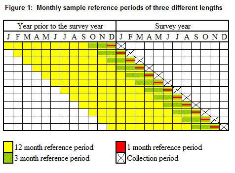
Description for Figure 1
This figure shows the sample reference periods of three different lengths for each of the twelve monthly collection periods from January to December.
For each monthly collection period, expenditures with a one-month reference period cover the month preceding the month of the collection period, expenditures with a three-month reference period cover the three months preceding the month of the collection period, and expenditures with a twelve-month reference period cover the twelve months preceding the month of the collection period. The following examples are based on the collection periods of January and December.
For the collection period of January of the survey year, expenditures with a one-month reference period cover the month of December of the year prior to the survey year, expenditures with a three-month reference period cover the period from October to December of the year prior to the survey year, and expenditures with a twelve-month reference period cover the period from January to December of the year prior to the survey year.
For the collection period of December of the survey year, expenditures with a one-month reference period cover the month of November of the survey year, expenditures with a three-month reference period cover the period from September to November of the survey year, and expenditures with a twelve-month reference period cover the period from December of the year prior to the survey year to November of the survey year.
Collected expenditures with a reference period of less than 12 months are annualized so that all expenditure amounts cover a period of 12 months. SHS estimates are produced by combining the data from the 12 monthly samples.
For annualized data from the 12 monthly samples that were combined to generate annual expenditure estimates (for expenditures with a recall period of 3 months or less), most of the expenditures were incurred during the survey reference year. This is also true for all expenditure data collected with the diary.
For expenditure items with a 12-month recall period, the collected expenses occurred between January of the year before the survey year and November of the survey year, depending on the collection month. For example, expenses collected in January cover the period from January to December of the year before the survey year, while expenses collected in December occurred between December of the year before the survey year and November of the survey year. For the estimates produced to represent a single 12-month period when the data from 12 monthly samples are combined, it must be assumed that expenditures incurred during the survey year are similar to those incurred during the previous year. This must be considered when making comparisons between estimates based on a 12-month recall period and those based on shorter periods.
The limits of the collection model used in producing expenditure estimates covering the same period (or the same year) are known, since the majority of countries use this methodology. Despite these limitations, continuous collection with reference periods adapted to the respondent’s ability to provide information is considered preferable to obtain data that reflect households’ true expenditures.
3.9 Comparability over time
The SHS has been conducted annually since 1997. This survey includes most of the content of its predecessors (the periodic Family Expenditure Survey and the Household Facilities and Equipment Survey). Prior to 2010, the SHS was primarily based on an interview during the first quarter of the year in which households reported expenditures incurred in the preceding calendar year, although some changes to the methodology and definitions were made between 1997 and 2009.
A new methodology, which combines a questionnaire and a diary to collect household expenditures, was introduced in the 10 provinces starting with the 2010 SHS. The recall periods have been shortened for several expenditure items and collection is now continuous throughout the year. Although the expenditure categories in the redesigned SHS are similar to those of previous years, the changes to data collection, processing and estimation methods have created a break in the data series. As a result, users are advised not to compare SHS data from 2010 onward with data prior to 2010, unless indicated otherwise.
The redesigned SHS incorporates a significant amount of content that was previously collected through the Food Expenditure Survey (FES), last conducted in 2001. Although there are some differences between the SHS and FES methodologies, food expenditure data in both surveys have been collected using an expenditure diary that households are asked to fill in for a period of two weeks. The content of the SHS diary is slightly less detailed than that of the FES diary (e.g., the weight and quantity of food items are not collected) in order to limit the SHS respondent’s burden.
The content of the SHS was also reviewed in 2010 to reduce the time required for the interview. A number of components regarding household equipment and dwelling characteristics as well as most of the questions regarding changes in household assets and liabilities have been dropped. Some definitions have also changed. As well, starting with the 2010 survey, the data related to household income and income tax come mainly from personal income tax data.
The new SHS design (applied in the 10 provinces since 2010) was introduced in the territories for the first time in the 2015 reference year. In prior years, coverage in the territories was near-complete and only remote communities were excluded. Starting in 2015, coverage in the three territories is limited to the capital cities due to operational and budget constraints as a result of adopting the new SHS design. As such, users are advised not to compare data for the territories from 2015 and later with those from previous years, unless otherwise noted.
Finally, for the 2010 to 2017 reference years, SHS estimates are based on weights calibrated to population estimates produced using data from the 2011 Census.
4. Data quality
Like all surveys, the SHS is subject to error, despite all the precautions taken in each step of the survey to prevent errors or reduce their impact. There are two types of errors: sampling and non-sampling.
4.1 Sampling errors
Sampling errors occur because inferences about the entire population are based on information obtained from only a sample of the population. The sample design, estimation method, sample size and data variability determine the size of the sampling error. The data variability for an expenditure item refers to the differences between members of the population in spending on that item. In general, the greater the differences between households, the larger the sampling error will be.
A common measure of sampling errors is the standard error (SE). The SE is the degree of variation in the estimates that results from selecting one particular sample over another. The SE expressed as a percentage of the estimate is called the coefficient of variation (CV). The CV is used to indicate the degree of uncertainty associated with an estimate. For example, if the estimated number of households with a given dwelling characteristic is 10,000 with a CV of 5%, then the actual number is between 9,500 and 10,500 households 68% of the time, and between 9,000 and 11,000 households 95% of the time.
The standard errors for the SHS are estimated using the bootstrap method (see reference [1] in Section 7). CVs are available for the national and provincial estimates as well as for the estimates by household type, age of reference person, household income quintile, household tenure and size of area of residence. For the northern territories, CVs are available for the estimates for the three capitals.
4.2 Data suppression
To ensure accuracy, estimates with a CV greater than or equal to 35% have been suppressed from published tables. Suppressed estimates still contribute to summary-level estimates. For example, if the expenditure estimate for a particular item of clothing were suppressed, this amount would still be included in the total estimate for clothing expenditure.
4.3 Non-sampling errors
Non-sampling errors occur because certain factors make it difficult to obtain accurate responses and to ensure that these responses retain their accuracy throughout processing. Unlike sampling errors, non-sampling errors are not easily quantified. Four sources of non-sampling errors can be identified: coverage errors, response errors, non‑response errors and processing errors.
4.3.1 Coverage errors
Coverage errors arise when sampling frame units do not adequately represent the target population. Such errors may occur during sample design or selection, or during data collection or processing.
4.3.2 Response errors
Response errors occur when respondents provide inaccurate information. Such errors may be due to many factors, including flawed design of the questionnaire, misinterpretation of questions by interviewers or respondents, or faulty reporting by respondents.
Response errors are the most difficult aspect of data quality to measure. In general, the accuracy of SHS data depends largely on the respondent’s ability to remember (recall) household expenditures and their willingness to consult records.
4.3.3 Non‑response errors
Errors due to non‑response occur when potential respondents do not provide the required information or when the information they provide is unusable. The main impact of non-response on data quality is that it can cause a bias in the estimates if the characteristics of non-respondents differ from those of respondents in a way that impacts the expenditures studied. While response rates can be calculated, they provide only an indication of data quality, since they do not measure the degree of bias present in the estimates. The magnitude of non-response can be considered a simple indicator of the risks of bias in the estimates.
At the national level (10 provinces only), the response rate for the 2017 SHS interview is 66.9%. The provincial response rates are shown in Table 1a. The table also shows the number of non-responding households grouped according to reason for non-response. Reasons include the inability to contact the household, the household’s refusal to participate in the survey and the inability to conduct an interview because of special circumstances (e.g., the respondent speaks neither official language or has a physical condition that precludes an interview). Respondents in the latter category are referred to as residual non‑respondents.
| Eligible sampled households | No contacts | Refusals | Residual non-respondents | Respondents | Response rateTable 1a Note 2 | |
|---|---|---|---|---|---|---|
| number | percentage | |||||
| Canada | 17,792 | 1,116 | 4,126 | 656 | 11,894 | 66.9 |
| Atlantic provinces | 5,738 | 357 | 1,259 | 252 | 3,870 | 67.4 |
| Newfoundland and Labrador | 1,577 | 124 | 321 | 47 | 1,085 | 68.8 |
| Prince Edward Island | 797 | 33 | 200 | 34 | 530 | 66.5 |
| Nova Scotia | 1,736 | 96 | 400 | 71 | 1,169 | 67.3 |
| New Brunswick | 1,628 | 104 | 338 | 100 | 1,086 | 66.7 |
| Quebec | 2,284 | 147 | 449 | 65 | 1,623 | 71.1 |
| Ontario | 2,562 | 128 | 672 | 125 | 1,637 | 63.9 |
| Prairie provinces | 5,033 | 324 | 1,241 | 130 | 3,338 | 66.3 |
| Manitoba | 1,671 | 112 | 385 | 57 | 1,117 | 66.8 |
| Saskatchewan | 1,628 | 102 | 442 | 26 | 1,058 | 65.0 |
| Alberta | 1,734 | 110 | 414 | 47 | 1,163 | 67.1 |
| British Columbia | 2,175 | 160 | 505 | 84 | 1,426 | 65.6 |
|
||||||
Some of the households selected to fill out a diary do not complete it or provide a diary that is considered unusable under the criteria outlined in section 3.5. For the 2017 SHS, the diary response rate among the interview-respondent households who were selected to fill out a diary is 62.9% (at the national level, including the provinces only). Provincial rates are provided in Table A1 of Appendix A. The final diary response rate (defined as the percentage of usable diaries relative to the number of households selected to fill out the diary) is 41.3% at the national level, and provincial rates are shown in Table 2a.
| Eligible sampled householdsTable 2a Note 2 | Interview non-respondentsTable 2a Note 3 | DiariesTable 2a Note 4 | Response rateTable 2a Note 6 | |||
|---|---|---|---|---|---|---|
| RefusalTable 2a Note 5 | Unusable | Usable | ||||
| number | percentage | |||||
| Canada | 8,948 | 3,063 | 2,048 | 138 | 3,699 | 41.3 |
| Atlantic provinces | 2,878 | 968 | 672 | 60 | 1,178 | 40.9 |
| Newfoundland and Labrador | 788 | 269 | 170 | 18 | 331 | 42.0 |
| Prince Edward Island | 410 | 139 | 105 | 5 | 161 | 39.3 |
| Nova Scotia | 865 | 290 | 191 | 25 | 359 | 41.5 |
| New Brunswick | 815 | 270 | 206 | 12 | 327 | 40.1 |
| Quebec | 1,147 | 336 | 286 | 10 | 515 | 44.9 |
| Ontario | 1,287 | 457 | 301 | 13 | 516 | 40.1 |
| Prairie provinces | 2,549 | 905 | 514 | 40 | 1,090 | 42.8 |
| Manitoba | 848 | 313 | 161 | 12 | 362 | 42.7 |
| Saskatchewan | 840 | 286 | 156 | 16 | 382 | 45.5 |
| Alberta | 861 | 306 | 197 | 12 | 346 | 40.2 |
| British Columbia | 1,087 | 397 | 275 | 15 | 400 | 36.8 |
|
||||||
The response rates vary from month to month. For the 10 provinces, monthly response rates for the interview and diary can be found in tables B1 and B2 of Appendix B. Interview and diary response rates by size of area of residence and dwelling type are shown in tables C1, C2, C3 and C4 of Appendix C, respectively.
The diary response rates of interview respondents can be found in tables D1, D2, D3 and D4 of Appendix D, broken down by various household characteristics, including household type, household tenure, age of the reference person and before-tax income quintile for the 10 provinces.
The interview response rates in the three territorial capitals are given in Table 1b below. Altogether, the three territorial capitals have an interview response rate equal to 64.4% for SHS 2017.
| Eligible sampled households | No contacts | Refusals | Residual non-respondents | Respondents | Response rateTable 1b Note 1 | |
|---|---|---|---|---|---|---|
| number | percentage | |||||
| Territorial capitals | 929 | 105 | 204 | 22 | 598 | 64.4 |
| Whitehorse | 472 | 40 | 130 | 13 | 289 | 61.2 |
| Yellowknife | 287 | 53 | 51 | 4 | 179 | 62.4 |
| Iqaluit | 170 | 12 | 23 | 5 | 130 | 76.5 |
|
||||||
In the three territorial capitals, all households selected for the interview are also selected to fill out a diary. Like in the provinces, some households do not complete it or provide a diary that is considered unusable under the criteria outlined in section 3.5. For the 2017 SHS, the final diary response rate in the northern capitals is 33.7%, as shown in table 2b.
| Eligible sampled households | Interview non-respondentsTable 2b Note 1 | DiariesTable 2b Note 2 | Response rateTable 2b Note 4 | |||
|---|---|---|---|---|---|---|
| RefusalTable 2b Note 3 | Unusable | Usable | ||||
| number | percentage | |||||
| Territorial capitals | 929 | 331 | 279 | 6 | 313 | 33.7 |
| Whitehorse | 472 | 183 | 152 | 2 | 135 | 28.6 |
| Yellowknife | 287 | 108 | 80 | 2 | 97 | 33.8 |
| Iqaluit | 170 | 40 | 47 | 2 | 81 | 47.6 |
|
||||||
For the northern capitals, the diary response rates among interview respondents are given in Table H1 of Appendix H. The interview and diary response rates by quarter are provided in Tables H2 and H3 of Appendix H.
For all selected households (provinces and territorial capitals), cases for which the respondent fails to answer some of the questions are referred to as partial non-response. Imputing missing values compensates for this partial non-response. Various imputation rates are shown in section 4.3.5.
There are also cases in which a household fails to enter data in the diary for each of the 14 days as required. Adjustment factors are thus calculated to take these non‑responded days into consideration.
4.3.4 Processing errors
Processing errors may occur in any of the data processing stages, including data entry, coding, editing, imputation of partial non-response, weighting and tabulation. Steps taken to reduce processing errors are described in section 3.5.
4.3.5 Imputation of partial non-responses
The residual bias remaining after the imputation of partial non-responses is difficult to measure. Its magnitude depends on the imputation method’s ability to produce unbiased estimates. The imputation rates provide an indication of the magnitude of partial non‑response.
Partial interview non-response may result from a lack of information or from an invalid response to a question. The national and provincial percentages of households for which certain expenditure categories required imputation due to partial interview non-response are shown in Table 3a. These percentages are shown for the three territorial capitals in Table 3b. These percentages are presented by number of imputed expenditure variables per household (out of all consumer expenditure data collected during the interview). Each of these tables contains two series of results: one series including expenditures for communication services (telephone, cell phone and Internet), television services (via cable, a satellite dish or a phone line), satellite radio services, and home security services, and the other excluding these expenses. This distinction has been made because these services are increasingly being purchased as a package. Households are often billed for bundled services, making it difficult or impossible for them to provide separate expenditure amounts for each service. Therefore, the total amount paid for the package is allocated to individual services through imputation, which significantly increases the number of households for which expenditures must be imputed.
| Number of variables imputed Table 3a Note 2 (out of 188) |
Number of variables imputed Table 3a Note 3 (out of 193) |
|||||||
|---|---|---|---|---|---|---|---|---|
| 1 | 2 to 9 | 10 or more | Total | 1 | 2 to 9 | 10 or more | Total | |
| percentage | ||||||||
| Canada | 19.6 | 34.2 | 2.4 | 56.2 | 8.6 | 66.8 | 4.3 | 79.7 |
| Newfoundland and Labrador | 20.0 | 31.9 | 1.2 | 53.1 | 5.6 | 76.7 | 3.9 | 86.2 |
| Prince Edward Island | 22.5 | 32.1 | 2.5 | 57.0 | 7.0 | 71.1 | 3.8 | 81.9 |
| Nova Scotia | 22.0 | 33.3 | 1.8 | 57.1 | 8.4 | 70.4 | 3.3 | 82.0 |
| New Brunswick | 18.7 | 23.5 | 1.4 | 43.6 | 5.3 | 71.5 | 2.9 | 79.8 |
| Quebec | 18.7 | 33.1 | 2.1 | 53.9 | 5.4 | 74.0 | 3.8 | 83.2 |
| Ontario | 20.2 | 32.4 | 2.0 | 54.6 | 10.6 | 60.8 | 3.1 | 74.5 |
| Manitoba | 15.2 | 50.2 | 6.1 | 71.5 | 9.6 | 63.6 | 9.3 | 82.5 |
| Saskatchewan | 21.3 | 36.2 | 1.5 | 59.0 | 12.9 | 62.1 | 3.3 | 78.4 |
| Alberta | 16.9 | 41.6 | 2.7 | 61.1 | 10.1 | 58.8 | 5.4 | 74.3 |
| British Columbia | 21.6 | 28.9 | 2.7 | 53.2 | 10.1 | 62.1 | 4.8 | 77.0 |
|
||||||||
| Number of variables imputed Table 3b Note 1 (out of 188) |
Number of variables imputed Table 3b Note 2 (out of 193) |
|||||||
|---|---|---|---|---|---|---|---|---|
| 1 | 2 to 9 | 10 or more | Total | 1 | 2 to 9 | 10 or more | Total | |
| percentage | ||||||||
| Territorial capitals | 17.7 | 41.1 | 3.2 | 62.0 | 12.4 | 56.5 | 4.5 | 73.4 |
| Whitehorse | 19.7 | 38.8 | 3.1 | 61.6 | 14.5 | 55.0 | 4.5 | 74.0 |
| Yellowknife | 13.4 | 41.9 | 1.1 | 56.4 | 7.3 | 60.9 | 2.8 | 70.9 |
| Iqaluit | 19.2 | 45.4 | 6.2 | 70.8 | 14.6 | 53.8 | 6.9 | 75.4 |
|
||||||||
Users of expenditure estimates related to communication, television, satellite radio or home security services should therefore take the high level of imputation for the expenditure data into account when examining these individual services. A measure of the impact of imputation on each individual service has been produced in Table E1 of Appendix E for the provinces and in Table H4 of Appendix H for the territorial capitals. This measure represents the proportion of the total value of the estimate obtained from imputed data.
For expenditure data from the diaries, imputation is used primarily to assign a value when the amount of a reported expenditure is missing, to assign a list of expenditure items (with individual costs) when only the total cost is provided (e.g., to assign grocery items and their individual costs when the respondent has provided only the total amount of the grocery bill), or to assign an expenditure code that is more detailed than the one that could be assigned using the information from the respondent (e.g., the type of bakery product). The imputation rates for each of these three types of imputation are shown in Table F1 of Appendix F for Canada and in Table H5 of Appendix H for the three territorial capitals. Each rate represents the proportion of imputed items relative to all expenditure items from the diaries.
The risks of bias associated with the imputed data depend largely on the level of detail at which the SHS data are used. For example, food expenditure data in the SHS are produced at a high level of detail to meet the needs of Food Expenditure Survey (last conducted in 2001) users. Food expenditures are categorized using a hierarchical system of more than 200 expenditure codes. For some reported expenditure items, the food product may have been known (e.g., dairy products or even milk), but the level of detail required (e.g., skim milk, 1% milk or 2% milk) had to be imputed. This type of imputation creates a risk of bias only in expenditure estimates at a very detailed level. In other cases, however, almost no information on the type of expenditure was available before imputation (e.g., it was known only that the expenditure was for a good). When so little information is available, the risks of bias in the estimates of the expenditure categories are more significant.
Restaurant expenditures are reported using a slightly different format in the second section of the diary. Imputation is used primarily to assign a value when the total amount of the restaurant expenditure or the cost of alcoholic beverages is missing, or when the type of meal (breakfast, lunch, dinner or snack and beverage) has not been specified. The imputation rate for each of these three types of imputation is shown in Table F2 of Appendix F for Canada and in Tables H6 of Appendix H for the territorial capitals.
Lastly, households have the option of either providing receipts or recording their expenditure information in the diary. Table 4a shows the percentage of expenditures reported using each method for food expenditures, restaurant expenditures, and expenditures for other goods and services for Canada and the three territorial capitals respectively.
| Expenditure category | Transcriptions | Receipts |
|---|---|---|
| percentage | ||
| Food | 21.6 | 78.4 |
| Restaurant | 82.3 | 17.7 |
| Other goods and services | 44.8 | 55.2 |
|
||
| Expenditure category | Transcriptions | Receipts |
|---|---|---|
| percentage | ||
| Food | 15.9 | 84.1 |
| Restaurant | 73.2 | 26.8 |
| Other goods and services | 37.0 | 63.0 |
4.4 The effect of large values
For any sample, estimates of totals, averages and standard errors can be affected by the presence or absence of large values in the sample. Large values are more likely to arise from positively skewed populations. Such values are found in the SHS and are taken into account when the final estimates are generated.
5. Derivation of data tables
This section shows how the SHS data tables, previously known as CANSIM tables (see Section 6), have been derived. It then explains the calculations used most frequently to manipulate the data. Users are advised to refer to this section before undertaking data analysis.
As mentioned in section 3.6, two different sets of weights are necessary for the SHS: one set for the interview and another set for the diary. These two weights are used to derive different estimates using the survey data.
5.1 Estimates of number of households
Estimates are generated using two sets of weights: one for the interview and the other for the diary. Adjustments made during weighting ensure that the estimated number of households at the provincial level is the same for both sets of weights for the following domains:
- Household sizes of one, two, and three or more persons. In 2017, two exceptions were made in the diary. For both Prince Edward Island and Alberta, two household sizes are used (one person, and two or more persons).
- Household income groups defined according to provincial quintiles.
By default, the estimate of the number of households for any aggregation of these domains is the same for both sets of weights.
For any other domain, an estimate of the number of households may differ somewhat between the two sets of weights, depending on the reliability of these estimates. The estimated number of households in the SHS tables has been produced using interview weights, as opposed to diary weights. The average household size is also estimated using the interview weights.
The estimated number of households and the average household size of the various domains for which expenditure estimates are produced in data tables are available in tables G1 and G2 of Appendix G for Canada and the provinces and in Table H7 of Appendix H for the territorial capitals.
5.2 Estimates of average expenditures per household
Estimates based on both interview and diary expenditure data are produced in two steps: estimates are produced separately for the interview data and the diary data, and are then added together.
For estimates of average expenditures per household, the interview average expenditures per household are first calculated using the weighted sum of expenditure data obtained from the interview divided by the sum of the interview weights. Similarly, the diary average expenditures per household are estimated using the weighted sum of expenditure data obtained from the diary divided by the sum of the diary weights. The two components are then added together to obtain the average expenditures per household. For domains in which the estimated number of households differs between the two sets of weights, average expenditures per household derived using this method of combining both sets of weights do not exactly match the combined interview and diary weighted sum of expenditures divided by the estimated number of households produced using the interview weights. Nevertheless, the approach ensures that the sum of the average expenditures per household for all categories equals the average total expenditure per household.
5.3 Examples of expenditure estimates
This section includes examples of expenditure estimates produced using a combination of interview and diary data. It also shows examples of the estimated number of households produced from the interview weights. These examples are provided to show how different expenditure estimates (presented in section 5.4) can be calculated using published SHS data.
The data tables available online include estimates of average expenditures per household. The estimated number of households and the average household size are also available at the national, regional and provincial levels. The estimated number of households and the average household size for other domains are not included in these tables, but are provided in tables G1 and G2 of Appendix G for Canada and the provinces and in Tables H7 of Appendix H for the three territorial capitals.
Table 5 shows the estimated number of households and average household size by household tenure as provided in the tables of Appendix G (not available in the data tables online), while Table 6 shows examples of average household expenditure estimates available to users through the SHS data tables.
| All households | Owner with mortgage | Owner without mortgage | Renter | |
|---|---|---|---|---|
| number | ||||
| Estimated number of households | 14,442,670 | 5,245,993 | 4,338,704 | 4,857,973 |
| Average household size | 2.47 | 3 | 2.2 | 2.14 |
| Note: Estimates in these tables are from the 2017 SHS and were calculated using weights based on population projections from the 2011 Census. | ||||
| All households | Owner with mortgage | Owner without mortgage | Renter | |
|---|---|---|---|---|
| dollars | ||||
| Total expendituresTable 6 Note 1 | 45,615 | 61,184 | 40,307 | 33,553 |
| Food expenditures | 8,527 | 9,899 | 8,720 | 6,871 |
| Food purchased from stores | 5,934 | 6,743 | 6,260 | 4,778 |
| Food purchased from restaurants | 2,593 | 3,156 | 2,460 | 2,092 |
| Shelter | 18,637 | 27,765 | 12,594 | 14,176 |
| Household furnishings and equipment | 2,314 | 3,068 | 2,517 | 1,327 |
| Clothing and accessories | 3,430 | 4,263 | 3,195 | 2,742 |
| Transportation | 12,707 | 16,189 | 13,281 | 8,437 |
|
||||
Tables 5 and 6 above are not available to users; however, the following section provides examples demonstrating how to produce other estimates using tables such as tables 7 and 8 above.
5.4 Calculating various estimates
The following section explains some of the calculation methods most commonly used to manipulate SHS expenditure estimates.
5.4.1 Average expenditures per person
To calculate the average expenditures per person for a given category, divide the average expenditures per household for that category (Table 6) by the average household size (found on the second line of Table 5). For example, the average food expenditures per person for renter households are calculated as follows:
Example:
When analyzing estimates of average expenditures per person, note that household composition (number of children and adults) is a significant factor in many expenditure patterns. As such, the method above provides only an approximation of the average per person. The SHS is not specifically designed to produce estimates of spending at the person level.
5.4.2 Percentage of average total household expenditures (budget share)
To calculate the budget share of an individual expenditure category as a percentage of average total household expenditures, divide the average expenditures per household for that category by the average total expenditures per household, and then multiply by 100. For example, using Table 6, the percentage of average total expenditures per household represented by the average expenditures on food per household, for renter households, is calculated by the following ratio:
Example:
5.4.3 Combining expenditure categories
The average expenditures per household for different expenditure categories can be added together in one column to create new subtotals. For example, the average expenditures on shelter and transportation combined per renter household are calculated as follows:
Example:
5.4.4 Aggregate expenditures
To calculate aggregate expenditures, multiply the average expenditures per household from one column for an expenditure category (Table 6) by the estimated number of households from the same column in Table 5. For example, the aggregate expenditures on food for renter households are calculated as follows:
Example:
Note: Since the average food expenditure comes from diary data alone, and the estimated number of households in the domain used differs slightly depending on whether it is calculated using the interview weights or the diary weights, this estimate of aggregate expenditures only approximates the value that would have been obtained using the weighted sum of expenditures. Indeed, if the estimated number of households used in the calculation were based on the diary weights (not available online), the estimate of aggregate food expenditures for renter households would be slightly different at $33,836,784,453.
The estimates of aggregate expenditures are exact for all domains for which the sum of the interview weights and the sum of the diary weights are the same (see section 5.1), as well as for all variables derived only from the interview.
5.4.5 Aggregate expenditures by combining data columns
To calculate aggregate expenditures for a given expenditure category for multiple columns, calculate the aggregate expenditures for this category for each column and then add them together.
For example, the aggregate expenditures on food by owner households (with or without a mortgage) are calculated as follows:
Example:
5.4.6 Average expenditures per household by combining data columns
To calculate the average expenditures for a given expenditure category for multiple columns, calculate the aggregate expenditures for this category for each column, add them together, and then divide the total by the sum of the estimated number of households in those columns (Table 7). For example, the average expenditures on food per owner household (with or without a mortgage) are calculated as follows:
Example:
5.4.7 Expenditure share of a subgroup among all households
Here the expenditure share is the percentage of the aggregate expenditures for a given expenditure category that belongs to a particular subgroup of households (e.g., the percentage of all food expenditures made by renter households). It is calculated by deriving the household subgroup’s aggregate expenditures for the expenditure category and dividing it by the aggregate expenditure for that expenditure category for all households. The result is then multiplied by 100. For example, the percentage of food expenditures made by renter households is calculated as follows:Example:
6. Related products and services
6.1 Data tables (formerly CANSIM)
Previously, Statistics Canada data was available via CANSIM (the Canadian Socioeconomic Information Management System), a database consisting of multidimensional cross-sectional tables. CANSIM tables were replaced by data tables with the same or similar content. All the content previously available has been integrated into the new data tables.
Eight tables presenting annual information from the Survey of Household Spending are available for Canada and the provinces. Table 11-10-0222-01 presents detailed household expenditure estimates, while tables 11-10-0223-01 to 11-10-0227-01 present data according to household income quintile, household type, household tenure, size of area of residence and age of the reference person, respectively. Table 11-10-0228-01 presents information on dwelling characteristics and household equipment. Finally, Table 11-10-0125-01 provides detailed food expenditure estimates.
Two tables are available with SHS estimates for the three territorial capitals. Table 11-10-0233-01 presents household expenditure estimates, while Table 11-10-0234-01 presents information on dwelling characteristics and household equipment.
6.2 Custom tabulations
For clients with more specialized data needs, custom tabulations can be produced to their specifications on a cost- recovery basis under the terms of a contract (subject to confidentiality restrictions). Detailed aggregate data on household expenditures are also available on a custom basis.
7. References
[1] Charlebois, J. and G. Dubreuil. 2011. Variance Estimation for the Redesigned Survey of Household Spending. Proceedings of the Survey Methods Section, Statistical Society of Canada Annual Meeting, June 2011.
Appendices
Appendix A - Diary response rates among interview respondents, Canada and provinces
Appendix B - Response rates by collection month, Canada
Appendix C - Response rates by size of area of residence and by dwelling type, Canada
Appendix G - Estimated number of households and average household size by domain, Canada
- Date modified: