Strategies for subsampling nonrespondents for economic programs
Section 3. Case study
This section presents the results of a simulation study
that evaluates the considered allocation procedures on empirical sample data
from the Annual Survey of Manufactures (ASM) from the 2010 and 2011 data
collections. For more information on the ASM, see
http://www.census.gov/manufacturing/asm.
The ASM is an establishment survey designed to produce
“sample estimates of statistics for all manufacturing establishments with one
or more paid employee(s)” (http://www.census.gov/manufacturing/ asm/); it is a
Pareto-PPS sample of approximately 50,000 establishments selected from a
universe of 328,500. Approximately 20,000 establishments are included with
certainty, and the remaining establishments are selected with probability
proportional to a composite measure of size. Selected units are in the sample
for the four years between censuses. Sampling strata are defined by six-digit
industry code using the North American Industry Classification System.
The ASM estimates totals with a difference estimator (Särndal
et al., 1992). To reduce respondent burden, units below a certain
threshold are dropped from the sampling frame entirely. Instead, their data are
imputed using administrative data values for selected items and industry-level
regression models for the remaining items. Similarly, the ASM imputes complete
records for unit nonrespondents. See http://www.census.gov/manufacturing/asm/
for additional information on the ASM methodology.
Because the items collected by the ASM questionnaire are
a subset of the EC’s manufacturing sector items, the ASM is often used to
pretest new EC processing or data collection procedures. With the ASM and the
EC, implementing a probability subsample of nonrespondents for NRFU represents
a major procedural change. The ASM NRFU procedures are very similar to the EC
procedures. Because a given company can comprise several establishments, the
sets of multi-unit (MU) establishments corresponding to the company can be
designated for phone follow-up as well as other company completeness checks. In
contrast, the NRFU procedures for the single unit (SU) establishments
establishments with one location and parent
company
differ. The largest SU establishments are
included with certainty (sampled with probability = 1) and may
receive a personal phone call in selected domains. The sampled SU
establishments (“SU noncertainty establishments”) receive some reminders, but
are very unlikely to receive a personal phone call.
Our simulation study examines one of the fourteen key
ASM items and employs the double expansion estimate and the two ratio
estimators described in the Appendix, not the difference estimator used in ASM
production estimates. Consequently, our results should not be extrapolated to
the ASM.
3.1 Simulation study design
Our simulation study compares the statistical properties
of total shipment estimates obtained from the three considered nonrespondent
subsampling designs over repeated samples, using three different estimators. Our sampling frame of nonrespondents is
derived from the fully imputed 2011 ASM sample and is limited to the SU
noncertainty establishments so that the overall ASM publication reliability requirements
are maintained. The ratio estimators employ the sample-based values of annual
payroll as an auxiliary variable. This variable is highly correlated with total
shipments, but is subject to imputation. Note that we use the complete ASM sample (all MU and SU
establishments) for the allocations but present the relative bias and MSE
results for the subsampled domains (SU noncertainty establishments) only.
For the SU noncertainty establishments, the first NRFU
attempt
consisting of a reminder letter
is historically very effective, so
nonrespondent subsample selection occurs before the second NRFU attempt. The
second NRFU attempt is generally more expensive (historically a package
re-mail, although reminder letters via certified mail will be used in future
collections). Nonrespondent subsampling of SU noncertainty establishments
occurs after the second contact
attempt (i.e., after the first NRFU attempt).
To perform the simulation, we removed all MU
establishments and SU certainty establishments from the ASM sample data to
create a frame, and then independently repeated the following procedure 5,000
times for each allocation procedure:
- Using the estimated response
propensities provided in Table 3.1, randomly induce nonresponse into the
sample using a MAR response mechanism.
- Sort the induced
nonrespondents by sampling weight.
- Select a stratified systematic
sample using the nonrespondent domain subsampling rates for a given allocation
strategy.
- Simulate unit response for
each round of NRFU. Table 3.1 provides the conditional response
propensities used for each distinct NRFU contact phase. These statistics use
paradata from the 2010 and 2011 ASM collections (Fink and Lineback, 2013).
Hereafter, we refer to these conditional probabilities as “nonrespondent
conversion rates”. If the unit responded, the mode of response is randomly
assigned using historical frequencies provided by subject matter experts. After assigning response status/response
mode to each unit, compute cumulative collection cost, URR, and estimates.
- For each allocation, repeat Step 4 until
either ten rounds of follow-up have been conducted or the total budget has been
expended. If funds are exhausted within a round, then NRFU ceases. Given that
the fixed budget assumes that
of the original set of nonrespondents will receive
NRFU, the budget can be exhausted under full follow-up. The total budget is
never expended before ten rounds of NRFU with nonrespondent subsampling, as the
cost-per-unit of mailing a reminder letter is quite low. Our choice of a
maximum of ten rounds of NRFU in the simulation was subjective; the purpose was
to demonstrate that subsampling would facilitate additional contact efforts at
no additional cost.
Table 3.1
Nonrespondent conversion rates for noncertainty single unit establishments by NRFU contact round used for simulation
Table summary
This table displays the results of Nonrespondent conversion rates for noncertainty single unit establishments by NRFU contact round used for simulation. The information is grouped by Domain (appearing as row headers), Initial Response Probability and Nonrespondent Conversion Rates for a given Round of Nonresponse Follow-up (appearing as column headers).
| Domain |
Initial Response Probability |
Nonrespondent Conversion Rates for a given Round of Nonresponse Follow-up |
| 1 |
2 |
3 |
4 |
5 |
6 |
7 |
8 |
9 |
10 |
| 1 |
0.31 |
0.27 |
0.15 |
0.17 |
0.24 |
0.12 |
0.06 |
0.03 |
0.03 |
0.03 |
0.03 |
| 2 |
0.44 |
0.32 |
0.24 |
0.15 |
0.36 |
0.18 |
0.09 |
0.05 |
0.05 |
0.05 |
0.05 |
| 3 |
0.39 |
0.28 |
0.24 |
0.18 |
0.11 |
0.06 |
0.03 |
0.02 |
0.02 |
0.02 |
0.02 |
| 4 |
0.35 |
0.36 |
0.17 |
0.19 |
0.18 |
0.09 |
0.05 |
0.02 |
0.02 |
0.02 |
0.02 |
| 5 |
0.25 |
0.19 |
0.13 |
0.10 |
0.17 |
0.09 |
0.04 |
0.02 |
0.02 |
0.02 |
0.02 |
| 6 |
0.27 |
0.13 |
0.29 |
0.02 |
0.02 |
0.02 |
0.02 |
0.02 |
0.02 |
0.02 |
0.02 |
| 7 |
0.44 |
0.34 |
0.23 |
0.20 |
0.25 |
0.13 |
0.06 |
0.03 |
0.03 |
0.03 |
0.03 |
| 8 |
0.38 |
0.45 |
0.12 |
0.33 |
0.25 |
0.13 |
0.06 |
0.03 |
0.03 |
0.03 |
0.03 |
| 9 |
0.39 |
0.30 |
0.23 |
0.13 |
0.25 |
0.13 |
0.06 |
0.03 |
0.03 |
0.03 |
0.03 |
| 10 |
0.75 |
1.00 |
0.00 |
0.00 |
0.00 |
0.00 |
0.00 |
0.00 |
0.00 |
0.00 |
0.00 |
| 11 |
0.28 |
0.23 |
0.12 |
0.18 |
0.15 |
0.07 |
0.04 |
0.02 |
0.02 |
0.02 |
0.02 |
| 12 |
0.36 |
0.30 |
0.21 |
0.15 |
0.31 |
0.16 |
0.08 |
0.04 |
0.04 |
0.04 |
0.04 |
| 13 |
0.39 |
0.22 |
0.19 |
0.13 |
0.23 |
0.12 |
0.06 |
0.03 |
0.03 |
0.03 |
0.03 |
| 14 |
0.37 |
0.36 |
0.16 |
0.06 |
0.45 |
0.22 |
0.11 |
0.06 |
0.06 |
0.06 |
0.06 |
| 15 |
0.41 |
0.32 |
0.22 |
0.19 |
0.26 |
0.13 |
0.06 |
0.03 |
0.03 |
0.03 |
0.03 |
| 16 |
0.40 |
0.34 |
0.22 |
0.23 |
0.32 |
0.16 |
0.08 |
0.04 |
0.04 |
0.04 |
0.04 |
| 17 |
0.34 |
0.26 |
0.18 |
0.10 |
0.21 |
0.11 |
0.05 |
0.03 |
0.03 |
0.03 |
0.03 |
| 18 |
0.40 |
0.31 |
0.18 |
0.10 |
0.18 |
0.09 |
0.04 |
0.02 |
0.02 |
0.02 |
0.02 |
| 19 |
0.37 |
0.29 |
0.20 |
0.19 |
0.23 |
0.11 |
0.06 |
0.03 |
0.03 |
0.03 |
0.03 |
| 20 |
0.40 |
0.28 |
0.21 |
0.15 |
0.18 |
0.09 |
0.04 |
0.02 |
0.02 |
0.02 |
0.02 |
| 21 |
0.36 |
0.27 |
0.20 |
0.14 |
0.23 |
0.11 |
0.06 |
0.03 |
0.03 |
0.03 |
0.03 |
The nonrespondent conversion rates in the majority of
domains follow the same pattern: a decaying response probability followed by a
slight increase in the fourth round due to a longer collection period. Domain
10 does not follow this pattern; it contained only four units that all
responded before subsampling began. After the 4th round of NRFU, the nonrespondent
conversion rates are reduced by half until they achieve the minimum allowable
value of 0.02. The pattern reflects the findings of Olson and Groves (2012).
(Olson and Groves (2012) postulate that the response propensities change over
the collection cycle, especially as data collection protocols are modified.
With the ASM, the reminder letters become more stringent at each NRFU contact
phase. Likewise, the authors demonstrate that response propensities decline
over the collection phase when a stable data collection protocol is used, as
reflected in nonrespondent conversion rates). Mail and phone response
propensity estimates were provided by subject matter experts,
as were approximate costs by mode and an overall budget figure.
To evaluate the statistical properties of
each allocation method for each estimator, we computed the
relative bias and the mean squared error. The relative bias (RBE) for each
estimate of total shipments at NRFU phase
for a given sampling overall interval
allocation method
eventual response probability
and estimator
(DE, SR, CR) is
where
is the estimated total and
is the population total shipments value.
The mean squared error at NRFU phase
for a given sampling interval, allocation
method and estimator is
Since our
simulation induces MAR response, the DE estimates should be approximately
unbiased over repeated samples, whereas the two ratio estimates should not be.
However, the DE estimates are expected to have large variance; using ratio
estimators with a positively correlated auxiliary variable is expected to
reduce this variance (i.e., increase the precision). Thus, examining the MSE
provides insight into the bias-variance tradeoff.
3.2 Allocation
The simulation study uses data from the 2011 ASM
collection. Input parameters for allocation were estimated from 2010 ASM
collection data. Recall that the target URR applies to the entire ASM program
and is not restricted to the subsampling domains - in our case, SU noncertainty
establishments. Consequently, the certainty SU and MU unit counts obtained from
the 2010 ASM data are included in the allocation programs in the
as constants; the remainder of the
represents the estimated count of responding
SU noncertainty establishments after the first round of NRFU is completed. To
ensure that each nonrespondent sampling domain contained sufficient numbers of
units to obtain a feasible solution, we used three-digit industry as NRFU
sampling domain instead of the six-digit industry used for the ASM sample
design [Note: the determination subsampling domain was determined collaborative
with the ASM program managers and methodologists].
Both
quadratic programs require an estimated probability of eventually responding to
follow-up
to compute the
(overall and by domain). To assess the
sensitivity of the allocation procedure, we tested ten different constant
values
keeping the value constant across all domains.
A similar approach can be taken when historic paradata are not available. In
addition, we estimate the
directly from the 2010 ASM data. These
estimates vary by 20-percent at three-digit industry level. However, the median
of these is nearly 50-percent. Consequently, the allocation obtained using the
estimated (historic-data)
values are very similar to those obtained with
Approximately
$21,000 was allotted for NRFU of SU noncertainty establishments after
subsampling. With full follow-up, the expected final unit response rate was
approximately 79%. Using data from the 2007 EC, Bechtel and Thompson (2013) found
that the target industry unit response rates of 70% could only be achieved in a
subsample if the average unit response rate in
the majority of EC industries was 60% or larger before follow-up begins. With the ASM, the response rate prior to
subsampling was approximately 57%. Instead, we select an overall
subsample, which would save approximately
50-percent of the allotted budget after five completed rounds of NRFU at the
cost of a decrease expected response rate (69%). The additional five rounds of
NRFU added approximately $4,000 to the total cost without commensurate
increases in response rate (70%). A larger subsample would be preferable in
terms of quality, but is not cost effective.
For
allocation, we obtain the
allowing the
to vary by domain. The maximum URR is always
achieved with the
quadratic program. Table 3.2 presents the
target URRs and the allocation subsampling rates obtained from the
quadratic program. A dash (-) indicates no
subsample is selected for NRFU (a sampling interval of
If
all units in the domain are selected for NRFU
(full follow-up). A label of
<value>
indicates that the eventual probability of respondent is the same constant
value in all domains; values estimated from historical data are labeled as
Est.
Recall that
includes all respondent units in the ASM
sample, not just the noncertainty single units that are eligible for
subsampling. Consequently, selected domains have achieved their target URRs before subsampling and are not
considered as subsampling candidates in the allocation programs.
As
the probability of eventually responding increases, this allocation tends to
select smaller subsamples in increasing numbers of domains. When the probability
of an eventual response
is small (20-percent or less), then the
allocations sensibly tend towards no subsampling or full follow-up, focusing on
obtaining sample from the few domains with the poorest response rates. As the probability
of an eventual response increases, the amount of subsampling tends to increase
as well. At 70-percent, almost half of the domains are allocated at least one
sampled unit, thus spreading the allocated sample across several domains
instead of concentrating in a few domains that have exceptionally poor response
rates. Note that rates below 20-percent are (hopefully) unrealistic as are
rates greater than 70-percent. Domain 10 has
highly variable sampling rates regardless; because all four units responded
before subsampling, the quadratic program selected any sampling rate because, in effect, it always subsamples zero
cases.
Table 3.2
Allocations (Sampling Intervals) (Program
Level
)
Table summary
This table displays the results of Allocations (Sampling Intervals) (Program Level . The information is grouped by Domain (appearing as row headers), (appearing as column headers).
| Domain |
|
| q = 10 |
q = 20 |
q = 30 |
q = 40 |
q = 50 |
q = 60 |
q = 70 |
q = 80 |
q = 90 |
q = 100 |
qh = Est |
| 1 |
- |
- |
- |
- |
- |
- |
- |
81.63 |
9.23 |
5.40 |
- |
| 2 |
- |
- |
- |
- |
- |
- |
3.88 |
2.26 |
1.71 |
1.44 |
- |
| 3 |
- |
- |
9.32 |
3.40 |
2.58 |
2.19 |
1.98 |
1.86 |
1.77 |
1.71 |
2.12 |
| 4 |
1.00 |
1.00 |
1.00 |
1.00 |
1.00 |
1.00 |
1.00 |
1.00 |
1.06 |
1.13 |
1.00 |
| 5 |
1.00 |
1.00 |
1.00 |
1.00 |
1.00 |
1.00 |
1.00 |
1.00 |
1.00 |
1.00 |
1.00 |
| 6 |
1.00 |
1.00 |
1.00 |
1.00 |
1.00 |
1.00 |
1.00 |
1.00 |
1.00 |
1.00 |
- |
| 7 |
- |
- |
- |
- |
- |
- |
- |
14.95 |
9.26 |
7.10 |
- |
| 8 |
- |
- |
- |
- |
- |
- |
- |
- |
- |
- |
- |
| 9 |
1.00 |
1.00 |
1.22 |
1.44 |
1.61 |
1.76 |
1.89 |
2.01 |
2.12 |
2.22 |
1.62 |
| 10 |
1.03 |
30.26 |
30.37 |
30.26 |
30.46 |
29.90 |
30.51 |
29.04 |
1.00 |
10.03 |
10.04 |
| 11 |
- |
- |
- |
- |
- |
- |
- |
- |
- |
- |
- |
| 12 |
- |
- |
- |
- |
- |
- |
- |
- |
- |
- |
- |
| 13 |
- |
- |
- |
- |
5.00 |
2.94 |
2.29 |
2.01 |
1.88 |
1.78 |
2.91 |
| 14 |
- |
- |
- |
- |
- |
- |
- |
- |
- |
- |
- |
| 15 |
7.86 |
4.45 |
3.22 |
2.57 |
2.42 |
2.32 |
2.28 |
2.30 |
2.35 |
2.40 |
2.38 |
| 16 |
1.00 |
1.35 |
1.46 |
1.46 |
1.49 |
1.51 |
1.53 |
1.57 |
1.62 |
1.66 |
1.66 |
| 17 |
1.00 |
1.00 |
1.00 |
1.00 |
1.00 |
1.00 |
1.00 |
1.00 |
1.00 |
1.00 |
1.00 |
| 18 |
- |
- |
- |
- |
- |
- |
- |
- |
- |
37.95 |
- |
| 19 |
1.00 |
1.00 |
1.00 |
1.00 |
1.00 |
1.00 |
1.00 |
1.00 |
1.00 |
1.00 |
1.00 |
| 20 |
1.00 |
1.00 |
1.00 |
1.16 |
1.34 |
1.49 |
1.63 |
1.75 |
1.87 |
1.97 |
1.35 |
| 21 |
1.00 |
1.00 |
1.00 |
1.00 |
1.00 |
1.00 |
1.00 |
1.00 |
1.00 |
1.00 |
1.00 |
|
72.5% |
72.9% |
73.3% |
73.7% |
74.1% |
74.4% |
74.8% |
75.2% |
75.6% |
76.0% |
74.3% |
Unlike
the
quadratic program, the
quadratic program did not always obtain a
solution for a given target URR because of the domain-level constraints on the
target URRs. When this occurred, we incrementally lowered the target response
rate until a feasible solution could be obtained. Table 3.3 presents the
target URRs and the allocations obtained from the
quadratic program.
Both
the allocation methods tend to designate the same domains for either no
subsampling or for full follow-up. However, the two methods produce very
different allocations for the same
in the subsampled domains. The
allocations avoid subsampling in domains that
have already achieved their maximum estimated target URR, regardless of the
probability of eventually obtaining a response, with 40- to 50-percent of the
domains not being subsampled when
Otherwise, the subsampling tends to be split
between full follow-up (all units selected) or subsampling at an approximately
sampling rate. In short, the
allocations yield domain subsampling intervals
that can differ considerably from the overall interval, as the allocation seeks
to equalize the target URR in each domain. The resultant variability in
sampling intervals can lead to large increases in sampling variance. Because
the
objective function seeks to equalize sampling
intervals, the domain subsampling intervals tend to be less variable and are
generally close to the overall sampling interval.
Table 3.3
Allocations (Sampling Intervals) (Program
Level
Table summary
This table displays the results of Allocations (Sampling Intervals) (Program Level . The information is grouped by Domain (appearing as row headers), (Target (appearing as column headers).
| Domain |
(Target ) |
| q = 10 |
q = 20 |
q = 30 |
q = 40 |
q = 50 |
q = 60 |
q = 70 |
q = 80 |
q = 90 |
q = 100 |
q = Est |
| 1 |
- |
- |
- |
- |
- |
- |
- |
- |
- |
- |
- |
| 2 |
- |
- |
- |
- |
- |
- |
- |
- |
2.00 |
2.00 |
- |
| 3 |
- |
- |
- |
- |
1.99 |
2.00 |
2.00 |
2.00 |
2.00 |
2.01 |
1.99 |
| 4 |
1.00 |
1.00 |
1.00 |
1.00 |
1.00 |
1.00 |
1.01 |
1.10 |
1.18 |
1.26 |
1.00 |
| 5 |
1.00 |
1.00 |
1.00 |
1.00 |
1.00 |
1.00 |
1.00 |
1.00 |
1.00 |
1.00 |
1.00 |
| 6 |
1.00 |
1.00 |
1.00 |
1.00 |
1.00 |
1.00 |
1.00 |
1.00 |
1.00 |
1.00 |
1.00 |
| 7 |
- |
- |
- |
- |
- |
- |
- |
- |
- |
2.06 |
- |
| 8 |
- |
- |
- |
- |
- |
- |
- |
- |
- |
- |
- |
| 9 |
1.00 |
1.32 |
1.44 |
1.72 |
1.90 |
1.99 |
1.97 |
1.96 |
1.96 |
2.09 |
1.90 |
| 10 |
- |
- |
- |
- |
- |
- |
- |
- |
- |
- |
- |
| 11 |
- |
- |
- |
- |
- |
- |
- |
- |
- |
- |
- |
| 12 |
- |
- |
- |
- |
- |
- |
- |
- |
- |
- |
- |
| 13 |
- |
- |
- |
- |
- |
1.99 |
1.99 |
1.98 |
1.98 |
2.04 |
- |
| 14 |
- |
- |
- |
- |
- |
- |
- |
- |
- |
- |
- |
| 15 |
2.52 |
2.23 |
2.36 |
1.90 |
1.76 |
1.97 |
1.92 |
1.90 |
1.90 |
2.27 |
1.76 |
| 16 |
2.17 |
2.08 |
1.71 |
1.83 |
1.90 |
1.97 |
1.97 |
1.96 |
1.96 |
2.09 |
1.90 |
| 17 |
1.00 |
1.00 |
1.00 |
1.00 |
1.00 |
1.00 |
1.00 |
1.00 |
1.00 |
1.00 |
1.00 |
| 18 |
- |
- |
- |
- |
- |
- |
- |
- |
- |
- |
- |
| 19 |
- |
2.01 |
1.00 |
1.00 |
1.00 |
1.00 |
1.00 |
1.00 |
1.00 |
1.00 |
1.00 |
| 20 |
1.00 |
1.00 |
1.11 |
1.36 |
1.57 |
1.75 |
1.90 |
1.97 |
1.97 |
2.06 |
1.59 |
| 21 |
1.00 |
1.00 |
1.00 |
1.00 |
1.00 |
1.00 |
1.00 |
1.00 |
1.00 |
1.00 |
1.00 |
|
71.0% |
71.4% |
72.3% |
72.7% |
73.1% |
73.4% |
73.8% |
74.2% |
74.6% |
75.0% |
73.3% |
3.3 Results
Our baseline closely mimics the NRFU procedures used in
the 2012 ASM NRFU
four phases of full follow-up
but can include an additional incomplete fifth
round when the planned budget was not depleted to retain programming
consistency. For other values of
NRFU is concluded after ten rounds regardless
of the remaining funds.
Table 3.4 presents the relative bias of the
estimates (RBE) and the mean squared error (MSE) results obtained with full
NRFU and the
allocation for each considered estimator. In
all cases, the unbiased double expansion (DE) estimator yields unbiased
estimates, whereas the ratio estimators are slightly biased as expected. With
subsampling, the relative bias of the ratio estimators increases, whereas the
DE estimator remains unbiased. Regardless of estimator, the additional stage of
subsampling increases the sampling variance and consequently the MSE; the bias
tends to remain unaffected because the subsampled units are a representative
subsample at each round of follow-up.
With equal probability subsampling
a subsample may contain a few sampled cases in
one or more domains. Although the subsampling weighting adjustment is not
variable, the nonresponse adjustment factors can be quite large. The optimal
allocations are designed to equalize response rates across domains, which can
lead to occasionally “oversampling” in low-responding domains. Table 3.5
presents the RBE and the MSE for the
optimal allocations, using three different
constant values of
and the domain specific rates estimated from
historical data
Estimated).
In all scenarios, the DE estimates are unbiased, the CR estimates are slightly
biased, and the SR estimates are the most biased. This repeats the RBE pattern
shown in the
allocation results. Moreover, the RBE
estimates do not appear to be overly sensitive to values of
used in allocation. Again, even with the
additional rounds of NRFU, the bias of the subsamples’ estimates is larger than
that obtained with full follow-up of nonrespondents. In all cases, the MSE of
the estimates obtained from the optimal allocations are smaller than those
obtained with the
allocations.
Regardless of estimator, the bias decreases when
eventually probability of responding is low. This seems a bit counterintuitive
but is in fact a direct consequence of the subsampling allocation procedure.
When the probability of obtaining an eventual response is low, the
allocation tends to subsample all or no units
in a domain. With full follow-up, all responding units within the same domain
have the same nonresponse adjustment. With a subsample, only the responding subsampled units’ weights are adjusted for
nonresponse and subsampling, in turn occasionally creating extremely variable
weights within domain. As the probability of an eventual response increases,
then the optimal allocation has sample in more domains, and finer adjustments
are possible. With that said, the CR estimators tend to produce the lowest
MSEs, regardless of allocation.
Table 3.4
Summary of relative bias in percent of the estimate and MSE for
allocations in x1012
Table summary
This table displays the results of Summary of relative bias in percent of the estimate and MSE for
allocations in x1012
Relative Bias of the Estimate,
Mean Squared Error, K = 1 (Full), K = 2, DE, CR and SR, calculated using Percent and x10^12 units of measure (appearing as column headers).
| Contact |
Relative Bias of the Estimate |
Mean Squared Error |
| Percent |
x10^12 |
| K = 1 (Full) |
K = 2 |
K = 1 (Full) |
K = 2 |
| DE |
CR |
SR |
DE |
CR |
SR |
DE |
CR |
SR |
DE |
CR |
SR |
| 2 |
0.01 |
0.03 |
0.10 |
0.00 |
0.51 |
1.43 |
4.96 |
2.60 |
5.56 |
37.53 |
26.34 |
70.49 |
| 3 |
0.00 |
0.03 |
0.08 |
-0.01 |
0.29 |
0.77 |
3.67 |
1.96 |
4.17 |
19.82 |
13.80 |
28.88 |
| 4 |
0.00 |
0.01 |
0.06 |
-0.02 |
0.14 |
0.40 |
2.55 |
1.39 |
3.03 |
11.75 |
8.30 |
14.87 |
| 5 |
0.01 |
0.02 |
0.04 |
-0.01 |
0.12 |
0.32 |
2.48 |
1.39 |
2.87 |
9.94 |
7.10 |
12.12 |
| 6 |
The is an empty cell |
The is an empty cell |
The is an empty cell |
-0.01 |
0.11 |
0.29 |
The is an empty cell |
The is an empty cell |
The is an empty cell |
9.36 |
6.75 |
11.16 |
| 7 |
The is an empty cell |
The is an empty cell |
The is an empty cell |
0.00 |
0.11 |
0.28 |
The is an empty cell |
The is an empty cell |
The is an empty cell |
9.09 |
6.63 |
10.63 |
| 8 |
The is an empty cell |
The is an empty cell |
The is an empty cell |
0.00 |
0.11 |
0.27 |
The is an empty cell |
The is an empty cell |
The is an empty cell |
8.80 |
6.48 |
10.23 |
| 9 |
The is an empty cell |
The is an empty cell |
The is an empty cell |
0.00 |
0.10 |
0.25 |
The is an empty cell |
The is an empty cell |
The is an empty cell |
8.51 |
6.32 |
9.95 |
| 10 |
The is an empty cell |
The is an empty cell |
The is an empty cell |
0.00 |
0.10 |
0.25 |
The is an empty cell |
The is an empty cell |
The is an empty cell |
8.27 |
6.19 |
9.74 |
Table 3.5
Summary of relative bias of the estimate and MSE for optimal allocations
Table summary
This table displays the results of Summary of relative bias of the estimate and MSE for optimal allocations. The information is grouped by Contact (appearing as row headers),
(Target , Percent, x10^12, q = 0.30, q = 0.50, q = 0.70 and q = Estimated (appearing as column headers).
| Contact |
(Target ) |
(Target ) |
| Percent |
x10^12 |
| q = 0.30 |
q = 0.50 |
q = 0.70 |
q = Estimated |
q = 0.30 |
q = 0.50 |
q = 0.70 |
q = Estimated |
| DE |
CR |
SR |
DE |
CR |
SR |
DE |
CR |
SR |
DE |
CR |
SR |
DE |
CR |
SR |
DE |
CR |
SR |
DE |
CR |
SR |
DE |
CR |
SR |
| 2 |
-0.01 |
0.06 |
0.20 |
0.01 |
0.07 |
0.36 |
0.01 |
0.08 |
0.31 |
-0.01 |
0.08 |
0.32 |
12.55 |
6.77 |
16.03 |
14.35 |
7.48 |
17.6 |
14.31 |
7.44 |
17.15 |
14.39 |
7.79 |
17.05 |
| 3 |
0.00 |
0.05 |
0.16 |
0.01 |
0.05 |
0.26 |
0.01 |
0.07 |
0.23 |
0.01 |
0.07 |
0.23 |
8.88 |
5.13 |
10.87 |
9.80 |
5.43 |
11.32 |
9.57 |
5.42 |
11.36 |
9.75 |
5.47 |
10.98 |
| 4 |
0.00 |
0.05 |
0.14 |
0.01 |
0.05 |
0.18 |
0.01 |
0.06 |
0.19 |
0.01 |
0.06 |
0.17 |
7.00 |
4.28 |
8.15 |
7.61 |
4.45 |
8.28 |
7.31 |
4.43 |
8.44 |
7.53 |
4.44 |
8.05 |
| 5 |
0.00 |
0.05 |
0.14 |
0.01 |
0.05 |
0.18 |
0.01 |
0.05 |
0.17 |
0.00 |
0.06 |
0.15 |
6.61 |
4.07 |
7.41 |
7.02 |
4.17 |
7.44 |
6.80 |
4.13 |
7.60 |
6.94 |
4.14 |
7.42 |
| 6 |
0.01 |
0.05 |
0.13 |
0.02 |
0.05 |
0.17 |
0.01 |
0.05 |
0.17 |
0.00 |
0.06 |
0.15 |
6.45 |
3.97 |
7.16 |
6.78 |
4.09 |
7.18 |
6.62 |
4.03 |
7.25 |
6.75 |
4.05 |
7.15 |
| 7 |
0.01 |
0.05 |
0.13 |
0.01 |
0.05 |
0.17 |
0.01 |
0.05 |
0.16 |
0.00 |
0.06 |
0.15 |
6.37 |
3.92 |
7.05 |
6.68 |
4.06 |
7.08 |
6.55 |
3.97 |
7.07 |
6.67 |
4.02 |
7.03 |
| 8 |
0.01 |
0.05 |
0.13 |
0.01 |
0.05 |
0.16 |
0.01 |
0.05 |
0.16 |
0.00 |
0.05 |
0.14 |
6.34 |
3.90 |
6.94 |
6.57 |
4.01 |
6.97 |
6.45 |
3.93 |
6.95 |
6.57 |
3.98 |
6.93 |
| 9 |
0.01 |
0.05 |
0.13 |
0.01 |
0.05 |
0.16 |
0.01 |
0.05 |
0.16 |
0.00 |
0.05 |
0.14 |
6.28 |
3.87 |
6.86 |
6.50 |
3.98 |
6.89 |
6.39 |
3.90 |
6.86 |
6.47 |
3.94 |
6.84 |
| 10 |
0.00 |
0.05 |
0.13 |
0.01 |
0.05 |
0.15 |
0.01 |
0.05 |
0.15 |
0.00 |
0.05 |
0.14 |
6.23 |
3.85 |
6.78 |
6.40 |
3.91 |
6.76 |
6.35 |
3.87 |
6.75 |
6.42 |
3.89 |
6.73 |
The
allocation procedure is designed to reduce the
variability in the subsampled units’ adjustment weights. Table 3.6
presents the relative bias of the estimate and MSE for the
optimal allocation method. The
estimators display the same pattern as before.
The DE estimates are unbiased, the CR estimates are nearly unbiased and the SR
estimates are slightly biased.
The MSE estimates for the
method follow a similar pattern as the
method, as expected due to the similarities
between corresponding
and
allocations. These results appear to be
relatively insensitive to assumed eventual probability of response
The historical-data estimated conversion rates
produce similar results to an assumed
0.50.
In many cases, the
method produces the least biased estimates.
However, bias is only a single component of the MSE, and the
allocations tend to have smaller expected
number of respondents in several strata than their
counterparts. Moreover, the
allocations have smaller sampling variances by
design, ultimately yielding estimates with lower MSEs than their
counterparts.
Figures 3.1 and 3.2 plot the RBEs and MSEs obtained
at each round of NRFU for the CR estimator (our “best” estimator) using the
obtained from historical data for each of the
considered optimal allocation methods along with the benchmark values (labeled
as “Full Follow-up”). In Figure 3.1, the benchmark estimates are the least
biased. However, this extremely low bias is in part a consequence of our
nonresponse model, which is uniform within domain and NRFU phase. Neither of
the optimal allocation estimates attained the benchmark estimate levels, but
they become very close after seven rounds of NRFU and the RBEs of the
and
CR estimates are less than one tenth of one percent (0.06% and
0.05% respectively). In summary, subsampling with either optimal allocation
strategy yielded trivial biases increases over full follow-up.
Table 3.6
Summary of relative bias of the estimate and MSE for optimal allocations
Table summary
This table displays the results of Summary of relative bias of the estimate and MSE for optimal allocations. The information is grouped by Contact (appearing as row headers), (Target , Percent, x10^12, q = 0.30, q = 0.50, q = 0.70 and q = Estimated (appearing as column headers).
| Contact |
(Target |
(Target |
| Percent |
x10^12 |
| q = 0.30 |
q = 0.50 |
q = 0.70 |
q = Estimated |
q = 0.30 |
q = 0.50 |
q = 0.70 |
q = Estimated |
| DE |
CR |
SR |
DE |
CR |
SR |
DE |
CR |
SR |
DE |
CR |
SR |
DE |
CR |
SR |
DE |
CR |
SR |
DE |
CR |
SR |
DE |
CR |
SR |
| 2 |
0.03 |
0.08 |
0.24 |
0.03 |
0.09 |
0.31 |
0.00 |
0.08 |
0.33 |
0.01 |
0.07 |
0.30 |
12.86 |
7.19 |
15.85 |
13.81 |
7.42 |
16.80 |
15.09 |
8.34 |
18.00 |
13.43 |
7.19 |
16.07 |
| 3 |
0.03 |
0.05 |
0.20 |
0.03 |
0.08 |
0.22 |
0.00 |
0.05 |
0.22 |
0.01 |
0.06 |
0.21 |
8.74 |
5.04 |
10.26 |
9.32 |
5.38 |
10.82 |
10.45 |
5.89 |
11.38 |
9.25 |
5.30 |
10.69 |
| 4 |
0.02 |
0.04 |
0.16 |
0.03 |
0.07 |
0.18 |
0.00 |
0.05 |
0.17 |
0.01 |
0.05 |
0.17 |
6.92 |
4.07 |
7.65 |
7.26 |
4.26 |
7.92 |
7.84 |
4.60 |
8.19 |
7.22 |
4.33 |
7.93 |
| 5 |
0.02 |
0.04 |
0.15 |
0.03 |
0.06 |
0.17 |
0.01 |
0.05 |
0.16 |
0.01 |
0.05 |
0.16 |
6.50 |
3.85 |
7.07 |
6.77 |
4.05 |
7.33 |
7.23 |
4.28 |
7.47 |
6.65 |
4.06 |
7.21 |
| 6 |
0.02 |
0.05 |
0.14 |
0.02 |
0.06 |
0.16 |
0.01 |
0.05 |
0.15 |
0.00 |
0.05 |
0.15 |
6.32 |
3.80 |
6.80 |
6.57 |
3.94 |
7.02 |
7.02 |
4.19 |
7.28 |
6.45 |
3.95 |
6.91 |
| 7 |
0.02 |
0.05 |
0.14 |
0.02 |
0.05 |
0.16 |
0.01 |
0.05 |
0.15 |
0.01 |
0.05 |
0.15 |
6.23 |
3.76 |
6.69 |
6.49 |
3.88 |
6.91 |
6.90 |
4.15 |
7.16 |
6.31 |
3.91 |
6.78 |
| 8 |
0.02 |
0.05 |
0.14 |
0.02 |
0.05 |
0.16 |
0.01 |
0.05 |
0.15 |
0.01 |
0.04 |
0.14 |
6.21 |
3.73 |
6.61 |
6.39 |
3.84 |
6.82 |
6.78 |
4.10 |
7.06 |
6.23 |
3.87 |
6.68 |
| 9 |
0.02 |
0.05 |
0.14 |
0.02 |
0.05 |
0.15 |
0.01 |
0.05 |
0.14 |
0.01 |
0.04 |
0.14 |
6.16 |
3.70 |
6.54 |
6.35 |
3.79 |
6.71 |
6.68 |
4.05 |
6.93 |
6.15 |
3.83 |
6.57 |
| 10 |
0.02 |
0.05 |
0.14 |
0.02 |
0.05 |
0.16 |
0.01 |
0.05 |
0.15 |
0.01 |
0.04 |
0.14 |
6.10 |
3.66 |
6.43 |
6.24 |
3.74 |
6.62 |
6.60 |
3.98 |
6.87 |
6.11 |
3.80 |
6.48 |
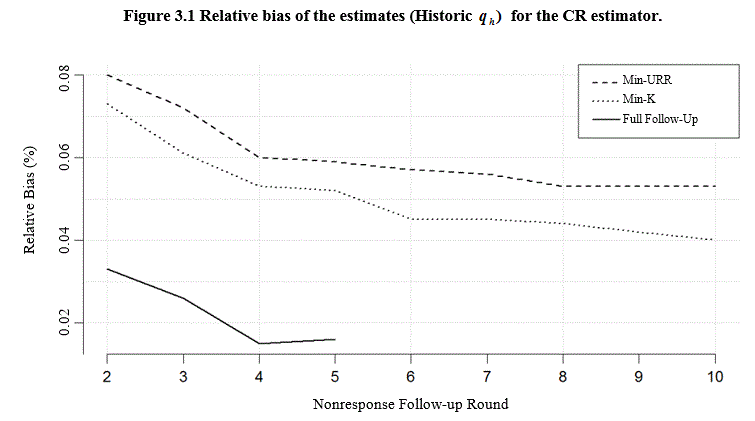
Description for Figure 3.1
Figure presenting the relative bias observed (Historic for the CR estimator, for each of the considered optimal allocation methods and along with the benchmark values (labeled as “Full Follow-up”). The relative bias, in percentage, is on the y-axis, ranging from 0.02 to 0.08. The nonresponse follow-up round is on the x-axis, ranging from 2 to 10. The benchmark estimates show the lowest relative bias. Estimates obtained with have a relative bias lower than the ones obtained from
Figure 3.2 plots MSE values by NRFU round using the
CR estimator. The targeted nonresponse sampling strategy used for the
allocation appears to reduce the overall
error. We believe that this is due to two factors. First, the
allocation procedure samples larger
proportions of nonrespondents in low responding areas than obtained with the
allocations. Second, the quadratic formula for
the
allocation includes a constraint on the domain
response rates, lowering the overall target response but reducing the
variability in the proportion of respondents by domain. Ultimately, this
approach yields similar response rates across sampling domains, indicative of a
representative sample (Wagner, 2012; Schouten, Cobben and Bethlehem, 2009).
Note that the increased MSE is not trivial with nonrespondent subsampling, even
when using an adjustment procedure that benefits from a strong covariate in the
ratio adjustment procedure. This is an acknowledged price paid for
nonrespondent subsampling (Biemer, 2010). However, this additional variance
component is measurable. If the measured component is too large, the program
managers can subsample less (use a larger
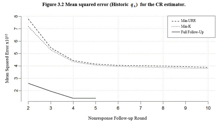
Description for Figure 3.2
Figure presenting the mean squared error observed (Historic for the CR estimator, for each of the considered optimal allocation methods and along with the benchmark values (labeled as “Full Follow-up”). The mean squared error (x 1012) is on the y-axis, ranging from 2 to 8. The nonresponse follow-up round is on the x-axis, ranging from 2 to 10. The benchmark estimates show the lowest MSE. Estimates obtained with have a MSE lower than the ones obtained from
3.4 Discussion
Given a sophisticated allocation method, a ratio
estimator employing a highly correlated auxiliary variable, and a fairly large
subsample, this case study shows that nonrespondent subsampling does not overly
penalize quality to save cost. The additional stage of sampling increased the
MSE for the studied variable, but the level was reduced by the judicious choice
of estimator. Of course, we consider only one variable in our simulation, and
this variable may or may not “behave” similarly to other survey items. One
referee suggested the usage of an R-indicator (Schouten et al., 2009) or
balance indicator (Särndal and Lundquist, 2014) to assess the overall
representativeness of the respondent sets in a field survey setting. This might
be useful at later stages of data collection (after nonrespondent subsampling
and during NRFU), but would not provide any further insight into the degree of
bias reduction on any collected item, as we can do in this simulation setting.
Of the three considered allocation methods, the
method had the worst performance, often
selecting a very small probability subsample when not needed and consequently
increasing the sampling variance without reducing the bias. Of the three
considered allocation methods, the
allocation was the most effective in realizing
acceptable response rates and achieving reliable estimates; the larger bias
caused by the varying domain sampling intervals is generally offset by the
reduced sampling variance. However, implementation of the
allocation can be more challenging than the
For both optimal allocation procedures, we tested four
different eventual probabilities of response to assess the sensitivity of the
allocation procedures to these inputs. By comparing allocations obtained with a
constant assumed input value to those obtained using the empirical estimates,
we found that the realized allocations could over- or under- sample in selected
domain, and the domain response rates could vary more than expected when the
actual (survey) values are quite different from the input values. Consequently,
we recommend using values estimated from historic paradata whenever possible.
If reducing cost is the overall goal, then we note that
additional NRFU contact attempts beyond the fifth contact did not improve the
bias or MSE of the subsampled estimates in our case study. Of course, if the
achieved cost reduction for a
subsample with up to ten NRFU contact attempts
is acceptable, the funds allocated to these final contact attempts might be
better expended earlier in the collection cycles using other contact
strategies.
