Strategies for subsampling nonrespondents for economic programs
Section 2. Methodology

2.1  Survey design and estimation

The general framework for our research is the two-phase sample design shown in Figure 2.1. The first stage is a stratified probability sample with a total sample size of n MathType@MTEF@5@5@+= feaagKart1ev2aqatCvAUfeBSjuyZL2yd9gzLbvyNv2CaerbuLwBLn hiov2DGi1BTfMBaeXatLxBI9gBaebbnrfifHhDYfgasaacH8rrps0l bbf9q8WrFfeuY=Hhbbf9y8WrFr0xc9vqFj0db9qqvqFr0dXdHiVc=b YP0xH8peuj0dYddrpe0db9Wqpepic9qr=xfr=xfr=xmeaabaqaciGa caGaaeqabaqaaeaadaaakeaacaWGUbaaaa@32B2@ from a finite population (frame) of size N , MathType@MTEF@5@5@+= feaagKart1ev2aqatCvAUfeBSjuyZL2yd9gzLbvyNv2CaerbuLwBLn hiov2DGi1BTfMBaeXatLxBI9gBaebbnrfifHhDYfgasaacH8rrps0l bbf9q8WrFfeuY=Hhbbf9y8WrFr0xc9vqFj0db9qqvqFr0dXdHiVc=b YP0xH8peuj0dYddrpe0db9Wqpepic9qr=xfr=xfr=xmeaabaqaciGa caGaaeqabaqaaeaadaaakeaacaWGobGaaiilaaaa@3342@ performed before data collection begins. The survey is conducted, and units either respond or do not. During the data collection, response rates are monitored in H MathType@MTEF@5@5@+= feaagKart1ev2aqatCvAUfeBSjuyZL2yd9gzLbvyNv2CaerbuLwBLn hiov2DGi1BTfMBaeXatLxBI9gBaebbnrfifHhDYfgasaacH8rrps0l bbf9q8WrFfeuY=Hhbbf9y8WrFr0xc9vqFj0db9qqvqFr0dXdHiVc=b YP0xH8peuj0dYddrpe0db9Wqpepic9qr=xfr=xfr=xmeaabaqaciGa caGaaeqabaqaaeaadaaakeaacaWGibaaaa@328C@ domains, where the domains do not necessarily equal the sampling strata. For example, total response rates might be monitored by three-digit industry classification, although these industry sampling strata are further broken down by size class. Furthermore, the domains could be independent of the original sampling strata e.g., race or sex categories (resembling post-strata). Hereafter, the term “domain” refers to the nonrespondent subsampling strata, indexed by h ( h = 1 , 2 , , H ) . MathType@MTEF@5@5@+= feaagKart1ev2aqatCvAUfeBSjuyZL2yd9gzLbvyNv2CaerbuLwBLn hiov2DGi1BTfMBaeXatLxBI9gBaebbnrfifHhDYfgasaacH8rrps0l bbf9q8WrFfeuY=Hhbbf9y8WrFr0xc9vqFj0db9qqvqFr0dXdHiVc=b YP0xH8peuj0dYddrpe0db9Wqpepic9qr=xfr=xfr=xmeaabaqaciGa caGaaeqabaqaaeaadaaakeaacaWGObWaaeWaaeaacaWGObGaeyypa0 JaaGymaiaacYcacaaIYaGaaiilaiablAciljaacYcacaWGibaacaGL OaGaayzkaaGaaiOlaaaa@3C50@

The second stage of probability sampling occurs at a predetermined point in the data collection cycle when we select an overall 1 in K MathType@MTEF@5@5@+= feaagKart1ev2aqatCvAUfeBSjuyZL2yd9gzLbvyNv2CaerbuLwBLn hiov2DGi1BTfMBaeXatLxBI9gBaebbnrfifHhDYfgasaacH8rrps0l bbf9q8WrFfeuY=Hhbbf9y8WrFr0xc9vqFj0db9qqvqFr0dXdHiVc=b YP0xH8peuj0dYddrpe0db9Wqpepic9qr=xfr=xfr=xmeaabaqaciGa caGaaeqabaqaaeaadaaakeaacaaIXaGaeyOeI0IaaeyAaiaab6gacq GHsislcaWGlbaaaa@3701@ subsample of size m 1 MathType@MTEF@5@5@+= feaagKart1ev2aqatCvAUfeBSjuyZL2yd9gzLbvyNv2CaerbuLwBLn hiov2DGi1BTfMBaeXatLxBI9gBaebbnrfifHhDYfgasaacH8rrps0l bbf9q8WrFfeuY=Hhbbf9y8WrFr0xc9vqFj0db9qqvqFr0dXdHiVc=b YP0xH8peuj0dYddrpe0db9Wqpepic9qr=xfr=xfr=xmeaabaqaciGa caGaaeqabaqaaeaadaaakeaacaWGTbWaaSbaaSqaaiaaigdaaeqaaa aa@3398@ from the m MathType@MTEF@5@5@+= feaagKart1ev2aqatCvAUfeBSjuyZL2yd9gzLbvyNv2CaerbuLwBLn hiov2DGi1BTfMBaeXatLxBI9gBaebbnrfifHhDYfgasaacH8rrps0l bbf9q8WrFfeuY=Hhbbf9y8WrFr0xc9vqFj0db9qqvqFr0dXdHiVc=b YP0xH8peuj0dYddrpe0db9Wqpepic9qr=xfr=xfr=xmeaabaqaciGa caGaaeqabaqaaeaadaaakeaacaWGTbaaaa@32B1@ nonrespondents (a two-phase sample); this predetermined point can be a fixed calendar date or via a responsive/adaptive design protocol. The value of K MathType@MTEF@5@5@+= feaagKart1ev2aqatCvAUfeBSjuyZL2yd9gzLbvyNv2CaerbuLwBLn hiov2DGi1BTfMBaeXatLxBI9gBaebbnrfifHhDYfgasaacH8rrps0l bbf9q8WrFfeuY=Hhbbf9y8WrFr0xc9vqFj0db9qqvqFr0dXdHiVc=b YP0xH8peuj0dYddrpe0db9Wqpepic9qr=xfr=xfr=xmeaabaqaciGa caGaaeqabaqaaeaadaaakeaacaWGlbaaaa@328F@ is determined by the program managers, who take into account the overall budget for NRFU (assumed fixed), mandated performance measures (e.g., response rates, coefficient of variation requirements), and other operational considerations such as length of collection period and available resources. Our allocation procedure determines the 1 in K h MathType@MTEF@5@5@+= feaagKart1ev2aqatCvAUfeBSjuyZL2yd9gzLbvyNv2CaerbuLwBLn hiov2DGi1BTfMBaeXatLxBI9gBaebbnrfifHhDYfgasaacH8rrps0l bbf9q8WrFfeuY=Hhbbf9y8WrFr0xc9vqFj0db9qqvqFr0dXdHiVc=b YP0xH8peuj0dYddrpe0db9Wqpepic9qr=xfr=xfr=xmeaabaqaciGa caGaaeqabaqaaeaadaaakeaacaaIXaGaeyOeI0IaaeyAaiaab6gacq GHsislcaWGlbWaaSbaaSqaaiaadIgaaeqaaaaa@381A@ systematic subsample of size m 1 h MathType@MTEF@5@5@+= feaagKart1ev2aqatCvAUfeBSjuyZL2yd9gzLbvyNv2CaerbuLwBLn hiov2DGi1BTfMBaeXatLxBI9gBaebbnrfifHhDYfgasaacH8rrps0l bbf9q8WrFfeuY=Hhbbf9y8WrFr0xc9vqFj0db9qqvqFr0dXdHiVc=b YP0xH8peuj0dYddrpe0db9Wqpepic9qr=xfr=xfr=xmeaabaqaciGa caGaaeqabaqaaeaadaaakeaacaWGTbWaaSbaaSqaaiaaigdacaWGOb aabeaaaaa@3485@ from the m h MathType@MTEF@5@5@+= feaagKart1ev2aqatCvAUfeBSjuyZL2yd9gzLbvyNv2CaerbuLwBLn hiov2DGi1BTfMBaeXatLxBI9gBaebbnrfifHhDYfgasaacH8rrps0l bbf9q8WrFfeuY=Hhbbf9y8WrFr0xc9vqFj0db9qqvqFr0dXdHiVc=b YP0xH8peuj0dYddrpe0db9Wqpepic9qr=xfr=xfr=xmeaabaqaciGa caGaaeqabaqaaeaadaaakeaacaWGTbWaaSbaaSqaaiaadIgaaeqaaa aa@33CA@ nonrespondents in each domain. Only the sampled m 1 h MathType@MTEF@5@5@+= feaagKart1ev2aqatCvAUfeBSjuyZL2yd9gzLbvyNv2CaerbuLwBLn hiov2DGi1BTfMBaeXatLxBI9gBaebbnrfifHhDYfgasaacH8rrps0l bbf9q8WrFfeuY=Hhbbf9y8WrFr0xc9vqFj0db9qqvqFr0dXdHiVc=b YP0xH8peuj0dYddrpe0db9Wqpepic9qr=xfr=xfr=xmeaabaqaciGa caGaaeqabaqaaeaadaaakeaacaWGTbWaaSbaaSqaaiaaigdacaWGOb aabeaaaaa@3485@ units receive NRFU.

Our objective is to estimate Y , MathType@MTEF@5@5@+= feaagKart1ev2aqatCvAUfeBSjuyZL2yd9gzLbvyNv2CaerbuLwBLn hiov2DGi1BTfMBaeXatLxBI9gBaebbnrfifHhDYfgasaacH8rrps0l bbf9q8WrFfeuY=Hhbbf9y8WrFr0xc9vqFj0db9qqvqFr0dXdHiVc=b YP0xH8peuj0dYddrpe0db9Wqpepic9qr=xfr=xfr=xmeaabaqaciGa caGaaeqabaqaaeaadaaakeaacaWGzbGaaiilaaaa@334D@ the population total of characteristic y . MathType@MTEF@5@5@+= feaagKart1ev2aqatCvAUfeBSjuyZL2yd9gzLbvyNv2CaerbuLwBLn hiov2DGi1BTfMBaeXatLxBI9gBaebbnrfifHhDYfgasaacH8rrps0l bbf9q8WrFfeuY=Hhbbf9y8WrFr0xc9vqFj0db9qqvqFr0dXdHiVc=b YP0xH8peuj0dYddrpe0db9Wqpepic9qr=xfr=xfr=xmeaabaqaciGa caGaaeqabaqaaeaadaaakeaacaWG5bGaaiOlaaaa@336F@ This estimate is Y ^ = Y ^ R 1 + Y ^ R 2 MathType@MTEF@5@5@+= feaagKart1ev2aqatCvAUfeBSjuyZL2yd9gzLbvyNv2CaerbuLwBLn hiov2DGi1BTfMBaeXatLxBI9gBaebbnrfifHhDYfgasaacH8rrps0l bbf9q8WrFfeuY=Hhbbf9y8WrFr0xc9vqFj0db9qqvqFr0dXdHiVc=b YP0xH8peuj0dYddrpe0db9Wqpepic9qr=xfr=xfr=xmeaabaqaciGa caGaaeqabaqaaeaadaaakeaaqaaaaaaaaaWdbiqadMfapaGbaKaape Gaeyypa0Jabmywa8aagaqcamaaBaaaleaapeGaamOuaiaaigdaa8aa beaak8qacqGHRaWkceWGzbWdayaajaWaaSbaaSqaa8qacaWGsbGaaG OmaaWdaeqaaaaa@3AA3@ where Y ^ R 1 MathType@MTEF@5@5@+= feaagKart1ev2aqatCvAUfeBSjuyZL2yd9gzLbvyNv2CaerbuLwBLn hiov2DGi1BTfMBaeXatLxBI9gBaebbnrfifHhDYfgasaacH8rrps0l bbf9q8WrFfeuY=Hhbbf9y8WrFr0xc9vqFj0db9qqvqFr0dXdHiVc=b YP0xH8peuj0dYddrpe0db9Wqpepic9qr=xfr=xfr=xmeaabaqaciGa caGaaeqabaqaaeaadaaakeaaqaaaaaaaaaWdbiqadMfapaGbaKaada WgaaWcbaWdbiaadkfacaaIXaaapaqabaaaaa@34B9@ is estimated from the r 1 h MathType@MTEF@5@5@+= feaagKart1ev2aqatCvAUfeBSjuyZL2yd9gzLbvyNv2CaerbuLwBLn hiov2DGi1BTfMBaeXatLxBI9gBaebbnrfifHhDYfgasaacH8rrps0l bbf9q8WrFfeuY=Hhbbf9y8WrFr0xc9vqFj0db9qqvqFr0dXdHiVc=b YP0xH8peuj0dYddrpe0db9Wqpepic9qr=xfr=xfr=xmeaabaqaciGa caGaaeqabaqaaeaadaaakeaaqaaaaaaaaaWdbiaadkhapaWaaSbaaS qaa8qacaaIXaGaamiAaaWdaeqaaaaa@34D8@ first-stage sample respondents and Y ^ R 2 MathType@MTEF@5@5@+= feaagKart1ev2aqatCvAUfeBSjuyZL2yd9gzLbvyNv2CaerbuLwBLn hiov2DGi1BTfMBaeXatLxBI9gBaebbnrfifHhDYfgasaacH8rrps0l bbf9q8WrFfeuY=Hhbbf9y8WrFr0xc9vqFj0db9qqvqFr0dXdHiVc=b YP0xH8peuj0dYddrpe0db9Wqpepic9qr=xfr=xfr=xmeaabaqaciGa caGaaeqabaqaaeaadaaakeaaqaaaaaaaaaWdbiqadMfapaGbaKaada WgaaWcbaWdbiaadkfacaaIYaaapaqabaaaaa@34BA@ is estimated from the r 2 h MathType@MTEF@5@5@+= feaagKart1ev2aqatCvAUfeBSjuyZL2yd9gzLbvyNv2CaerbuLwBLn hiov2DGi1BTfMBaeXatLxBI9gBaebbnrfifHhDYfgasaacH8rrps0l bbf9q8WrFfeuY=Hhbbf9y8WrFr0xc9vqFj0db9qqvqFr0dXdHiVc=b YP0xH8peuj0dYddrpe0db9Wqpepic9qr=xfr=xfr=xmeaabaqaciGa caGaaeqabaqaaeaadaaakeaaqaaaaaaaaaWdbiaadkhapaWaaSbaaS qaa8qacaaIYaGaamiAaaWdaeqaaaaa@34D9@ second-stage sample respondents (see Figure 2.1). Nonresponse adjustments to the r 2 h MathType@MTEF@5@5@+= feaagKart1ev2aqatCvAUfeBSjuyZL2yd9gzLbvyNv2CaerbuLwBLn hiov2DGi1BTfMBaeXatLxBI9gBaebbnrfifHhDYfgasaacH8rrps0l bbf9q8WrFfeuY=Hhbbf9y8WrFr0xc9vqFj0db9qqvqFr0dXdHiVc=b YP0xH8peuj0dYddrpe0db9Wqpepic9qr=xfr=xfr=xmeaabaqaciGa caGaaeqabaqaaeaadaaakeaaqaaaaaaaaaWdbiaadkhapaWaaSbaaS qaa8qacaaIYaGaamiAaaWdaeqaaaaa@34D9@ subsampled (responding) units assume a missing at random response (MAR) mechanism, treated as a Bernoulli sample (Särndal, Swensson and Wretman, 1992, Chapter 15; Kott, 1994). We consider three different adjustment-to-sample reweighting estimators of Y ^ R 2 MathType@MTEF@5@5@+= feaagKart1ev2aqatCvAUfeBSjuyZL2yd9gzLbvyNv2CaerbuLwBLn hiov2DGi1BTfMBaeXatLxBI9gBaebbnrfifHhDYfgasaacH8rrps0l bbf9q8WrFfeuY=Hhbbf9y8WrFr0xc9vqFj0db9qqvqFr0dXdHiVc=b YP0xH8peuj0dYddrpe0db9Wqpepic9qr=xfr=xfr=xmeaabaqaciGa caGaaeqabaqaaeaadaaakeaaqaaaaaaaaaWdbiqadMfapaGbaKaada WgaaWcbaWdbiaadkfacaaIYaaapaqabaaaaa@34BA@ (Kalton and Flores-Cervantes, 2003): the double reweighted expansion (DE) estimator (Binder, Babyak, Brodeur, Hidiroglou and Wisner, 2000; Shao and Thompson, 2009; Haziza, Thompson and Yung, 2010), a separate ratio (SR) estimator that adjusts for unit nonresponse using a covariate that is highly correlated with both response propensity and the survey characteristic of interest (Shao and Thompson, 2009; Haziza et al., 2010), and a combined ratio (CR) estimator (Binder et al., 2000). Formulae are provided in the Appendix.

Figure 2.1 Nonrespondent subsample from probability sample, selected during data collection (two-phase sample design). Unsampled nonrespondents do not receive NRFU

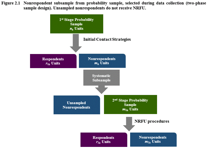
Description for Figure 2.1

Figure illustrating the two-phase sample design. First of all, a first stage probability sample is drawn (size n h ). MathType@MTEF@5@5@+= feaagKart1ev2aqatCvAUfeBSjuyZL2yd9gzLbvyNv2CaerbuLwBLn hiov2DGi1BTfMBaeXatLxBI9gBaerbd9wDYLwzYbItLDharqqtubsr 4rNCHbGeaGqipu0Je9sqqrpepC0xbbL8F4rqqrFfpeea0xe9Lq=Jc9 vqaqpepm0xbba9pwe9Q8fs0=yqaqpepae9pg0FirpepeKkFr0xfr=x fr=xb9adbaqaaeGaciGaaiaabeqaamaabaabaaGcbaGaamOBamaaBa aaleaacaWGObaabeaakiaacMcacaGGUaaaaa@394C@ Initial contact strategies are put in place. There are r 1h MathType@MTEF@5@5@+= feaagKart1ev2aqatCvAUfeBSjuyZL2yd9gzLbvyNv2CaerbuLwBLn hiov2DGi1BTfMBaeXatLxBI9gBaerbd9wDYLwzYbItLDharqqtubsr 4rNCHbGeaGqipu0Je9sqqrpepC0xbbL8F4rqqrFfpeea0xe9Lq=Jc9 vqaqpepm0xbba9pwe9Q8fs0=yqaqpepae9pg0FirpepeKkFr0xfr=x fr=xb9adbaqaaeGaciGaaiaabeqaamaabaabaaGcbaGaamOCamaaBa aaleaacaaIXaGaamiAaaqabaaaaa@38A2@ respondent to this first stage and m h MathType@MTEF@5@5@+= feaagKart1ev2aqatCvAUfeBSjuyZL2yd9gzLbvyNv2CaerbuLwBLn hiov2DGi1BTfMBaeXatLxBI9gBaerbd9wDYLwzYbItLDharqqtubsr 4rNCHbGeaGqipu0Je9sqqrpepC0xbbL8F4rqqrFfpeea0xe9Lq=Jc9 vqaqpepm0xbba9pwe9Q8fs0=yqaqpepae9pg0FirpepeKkFr0xfr=x fr=xb9adbaqaaeGaciGaaiaabeqaamaabaabaaGcbaGaamyBamaaBa aaleaacaWGObaabeaaaaa@37E2@ nonrespondents which will be subsampled using a systematic design. The size of this second stage probability sample is m 1h . MathType@MTEF@5@5@+= feaagKart1ev2aqatCvAUfeBSjuyZL2yd9gzLbvyNv2CaerbuLwBLn hiov2DGi1BTfMBaeXatLxBI9gBaerbd9wDYLwzYbItLDharqqtubsr 4rNCHbGeaGqipu0Je9sqqrpepC0xbbL8F4rqqrFfpeea0xe9Lq=Jc9 vqaqpepm0xbba9pwe9Q8fs0=yqaqpepae9pg0FirpepeKkFr0xfr=x fr=xb9adbaqaaeGaciGaaiaabeqaamaabaabaaGcbaGaamyBamaaBa aaleaacaaIXaGaamiAaaqabaGccaGGUaaaaa@3959@ These units receive the NRFU procedures. Among these sampled units, there are r 2h MathType@MTEF@5@5@+= feaagKart1ev2aqatCvAUfeBSjuyZL2yd9gzLbvyNv2CaerbuLwBLn hiov2DGi1BTfMBaeXatLxBI9gBaerbd9wDYLwzYbItLDharqqtubsr 4rNCHbGeaGqipu0Je9sqqrpepC0xbbL8F4rqqrFfpeea0xe9Lq=Jc9 vqaqpepm0xbba9pwe9Q8fs0=yqaqpepae9pg0FirpepeKkFr0xfr=x fr=xb9adbaqaaeGaciGaaiaabeqaamaabaabaaGcbaGaamOCamaaBa aaleaacaaIYaGaamiAaaqabaaaaa@38A3@ respondents and m 2h MathType@MTEF@5@5@+= feaagKart1ev2aqatCvAUfeBSjuyZL2yd9gzLbvyNv2CaerbuLwBLn hiov2DGi1BTfMBaeXatLxBI9gBaerbd9wDYLwzYbItLDharqqtubsr 4rNCHbGeaGqipu0Je9sqqrpepC0xbbL8F4rqqrFfpeea0xe9Lq=Jc9 vqaqpepm0xbba9pwe9Q8fs0=yqaqpepae9pg0FirpepeKkFr0xfr=x fr=xb9adbaqaaeGaciGaaiaabeqaamaabaabaaGcbaGaamyBamaaBa aaleaacaaIYaGaamiAaaqabaaaaa@389E@ nonrespondents.

These estimators require a minimum of r 2 h = 1 MathType@MTEF@5@5@+= feaagKart1ev2aqatCvAUfeBSjuyZL2yd9gzLbvyNv2CaerbuLwBLn hiov2DGi1BTfMBaeXatLxBI9gBaebbnrfifHhDYfgasaacH8rrps0l bbf9q8WrFfeuY=Hhbbf9y8WrFr0xc9vqFj0db9qqvqFr0dXdHiVc=b YP0xH8peuj0dYddrpe0db9Wqpepic9qr=xfr=xfr=xmeaabaqaciGa caGaaeqabaqaaeaadaaakeaacaWGYbWaaSbaaSqaaiaaikdacaWGOb aabeaakiabg2da9iaaigdaaaa@3656@ in each domain and a minimum of r 2 h = 2 MathType@MTEF@5@5@+= feaagKart1ev2aqatCvAUfeBSjuyZL2yd9gzLbvyNv2CaerbuLwBLn hiov2DGi1BTfMBaeXatLxBI9gBaebbnrfifHhDYfgasaacH8rrps0l bbf9q8WrFfeuY=Hhbbf9y8WrFr0xc9vqFj0db9qqvqFr0dXdHiVc=b YP0xH8peuj0dYddrpe0db9Wqpepic9qr=xfr=xfr=xmeaabaqaciGa caGaaeqabaqaaeaadaaakeaacaWGYbWaaSbaaSqaaiaaikdacaWGOb aabeaakiabg2da9iaaikdaaaa@3657@ for variance estimation. These minimal conditions may not hold for several reasons. During the early stages of NRFU collection, an insufficient number of the subsampled units might respond in a given domain. Alternatively, the allocation procedure could determine that no subsampling is required in one or more domains. Lastly, the allocation procedure could require 100-percent follow-up (all units subsampled) in selected domains; henceforth, we refer to 100-percent follow-up/no subsampling as “full follow-up”. In these cases, the estimation procedure ignores the last stage of sampling as if it did not occur and produces estimates for domain h MathType@MTEF@5@5@+= feaagKart1ev2aqatCvAUfeBSjuyZL2yd9gzLbvyNv2CaerbuLwBLn hiov2DGi1BTfMBaeXatLxBI9gBaebbnrfifHhDYfgasaacH8rrps0l bbf9q8WrFfeuY=Hhbbf9y8WrFr0xc9vqFj0db9qqvqFr0dXdHiVc=b YP0xH8peuj0dYddrpe0db9Wqpepic9qr=xfr=xfr=xmeaabaqaciGa caGaaeqabaqaaeaadaaakeaacaWGObaaaa@32AC@ using the collapsed estimator formulae provided in the Appendix.

2.2  Allocation strategies

When all nonresponding cases are subjected to NRFU, respondent contact strategies focus on improving overall response rates. Analysts might focus primarily on obtaining responses from soft refusal cases that they believe have similar characteristics to previous respondents (“quick wins”), although this phenomenon is more likely when the survey collection is performed in the field, as with household or agricultural surveys, and perhaps is less likely for internet or mail collections. With business surveys, the size of the unit is a factor in the NRFU procedures as discussed in Section 1.

Our objective is to obtain a realized set of respondents that approximates a random subsample of the originally selected sample via a probability sample of nonrespondents. With a probability sample, the targeted cases represent a cross-section of the nonrespondent population. By focusing contact efforts on the subsample, we hope to decrease the effects of nonresponse bias on the estimated totals by obtaining data from all types of nonresponding units. Moreover, weighting or imputation methods may be more effective at reducing the nonresponse bias effects with a probability subsample of nonrespondents (Brick, 2013). Even though they do not receive additional NRFU, the unsampled nonrespondent cases may provide responses later in the collection cycle. If so, an unbiased estimation procedure would not include the unsampled late responses in the final estimate assuming that all subsampled units respond, as these units are represented by the subsampled cases. However, this procedure is extremely distasteful to many survey managers. Instead, we include their data in the tabulations as if they had responded before subsampling. This does induce bias in the estimate. In practice, we ensure that this situation occurs infrequently by subsampling late in the data collection cycle.

With a business survey that keeps track of little or no demographic information, most of the information on the nonrespondents such as industry and unit size (e.g., total payroll, total receipts) is obtained from the sampling frame. Sorting the nonrespondents within prespecified domains by unit size and selecting a systematic sample should yield a subsample that resembles the originally designed sample in terms of unit size composition. This is especially important for business surveys where responses tend to be obtained from the larger units (Thompson and Washington, 2013). The choice of subsampling domain is determined by overall survey objectives such as publication levels or by the adjustment cell design (e.g., weighting cells or imputation classes), although computations are considerably simplified when the domain of interest is the original sampling strata. In the EC, the industry is the domain of interest.

We consider two allocation approaches: (1) equal-probability sampling; and (2) optimized allocation with constraints on unit response rates and sample size in predetermined domains. Equal probability sampling is easy to implement and should have the lowest sampling variance among considered nonrespondent subsampling allocation strategies, since the subsampling weight adjustment will be a constant value in all domains. However, since the same proportion of nonrespondents is sampled in each domain, the subsample may not be large enough to offset nonresponse bias effects on totals in low-responding domains. We refer to the allocations obtained by equal probability sampling as Constant K , MathType@MTEF@5@5@+= feaagKart1ev2aqatCvAUfeBSjuyZL2yd9gzLbvyNv2CaerbuLwBLn hiov2DGi1BTfMBaeXatLxBI9gBaebbnrfifHhDYfgasaacH8rrps0l bbf9q8WrFfeuY=Hhbbf9y8WrFr0xc9vqFj0db9qqvqFr0dXdHiVc=b YP0xH8peuj0dYddrpe0db9Wqpepic9qr=xfr=xfr=xmeaabaqaciGa caGaaeqabaqaaeaadaaakeaacaqGdbGaae4Baiaab6gacaqGZbGaae iDaiaabggacaqGUbGaaeiDaiaayIW7cqGHsislcaaMi8Uaam4saiaa cYcaaaa@3EB0@ where K MathType@MTEF@5@5@+= feaagKart1ev2aqatCvAUfeBSjuyZL2yd9gzLbvyNv2CaerbuLwBLn hiov2DGi1BTfMBaeXatLxBI9gBaebbnrfifHhDYfgasaacH8rrps0l bbf9q8WrFfeuY=Hhbbf9y8WrFr0xc9vqFj0db9qqvqFr0dXdHiVc=b YP0xH8peuj0dYddrpe0db9Wqpepic9qr=xfr=xfr=xmeaabaqaciGa caGaaeqabaqaaeaadaaakeaacaWGlbaaaa@328F@ refers to the overall sampling interval ( 1 in K ) . MathType@MTEF@5@5@+= feaagKart1ev2aqatCvAUfeBSjuyZL2yd9gzLbvyNv2CaerbuLwBLn hiov2DGi1BTfMBaeXatLxBI9gBaebbnrfifHhDYfgasaacH8rrps0l bbf9q8WrFfeuY=Hhbbf9y8WrFr0xc9vqFj0db9qqvqFr0dXdHiVc=b YP0xH8peuj0dYddrpe0db9Wqpepic9qr=xfr=xfr=xmeaabaqaciGa caGaaeqabaqaaeaadaaakeaadaqadaqaaiaaigdacqGHsislcaqGPb GaaeOBaiabgkHiTiaadUeaaiaawIcacaGLPaaacaGGUaaaaa@393C@

Our optimized allocation methods address the above concern by concentrating NRFU efforts in domains that have low response rates, attempting to select sufficient cases to achieve the performance benchmarks. This strategy may decrease the nonresponse bias in the totals if the response mechanism is MAR, conditional on the auxiliary variables used to define the domains; see Wagner (2012). However, it can increase the variance, as the subsampling intervals will differ and the weights will become more variable. To minimize the additional sampling variance caused by differing sampling intervals, the domain nonrespondent subsampling intervals should be close to the overall nonrespondent subsampling interval. To control costs, the allocation should not select more units for NRFU than budgeted. Recall that the federal survey environment requires that target response rates be achieved or nearly achieved, which makes all domains “equally” important from a data collection viewpoint.

To describe the allocation procedures, we introduce additional notation:

Unit response rate:                   URR = h ( r 1 h + r 2 h ) h n h MathType@MTEF@5@5@+= feaagKart1ev2aaatCvAUfeBSjuyZL2yd9gzLbvyNv2CaerbuLwBLn hiov2DGi1BTfMBaeXatLxBI9gBaebbnrfifHhDYfgasaacH8rrps0l bbf9q8WrFfeuY=Hhbbf9y8WrFr0xc9vqFj0db9qqvqFr0dXdHiVc=b YP0xH8peuj0dYddrpe0db9Wqpepic9qr=xfr=xfr=xmeaabaqaciGa caGaaeqabaqaaeaadaaakeaacaqGvbGaaeOuaiaabkfacqGH9aqpda WcaaqaamaaqababaWaaeWaaeaaqaaaaaaaaaWdbiaadkhapaWaaSba aSqaa8qacaaIXaGaamiAaaWdaeqaaOWdbiabgUcaRiaadkhapaWaaS baaSqaa8qacaaIYaGaamiAaaWdaeqaaaGccaGLOaGaayzkaaaaleaa caWGObaabeqdcqGHris5aaGcbaWaaabeaeaapeGaamOBa8aadaWgaa WcbaWdbiaadIgaa8aabeaaaeaacaWGObaabeqdcqGHris5aaaaaaa@45E1@

Target response rate:                URR T = h r 1 h + ( q h m h / K ) h n h MathType@MTEF@5@5@+= feaagKart1ev2aaatCvAUfeBSjuyZL2yd9gzLbvyNv2CaerbuLwBLn hiov2DGi1BTfMBaeXatLxBI9gBaebbnrfifHhDYfgasaacH8rrps0l bbf9q8WrFfeuY=Hhbbf9y8WrFr0xc9vqFj0db9qqvqFr0dXdHiVc=b YP0xH8peuj0dYddrpe0db9Wqpepic9qr=xfr=xfr=xmeaabaqaciGa caGaaeqabaqaaeaadaaakeaacaqGvbGaaeOuaiaabkfadaahaaWcbe qaaiaabsfaaaGccqGH9aqpdaWcaaqaamaaqababaGaamOCamaaBaaa leaacaaIXaGaamiAaaqabaGccqGHRaWkdaqadaqaaabaaaaaaaaape WaaSGbaeaacaWGXbWaaSbaaSqaaiaadIgaaeqaaOGaamyBamaaBaaa leaacaWGObaabeaaaOqaaiaadUeaaaaapaGaayjkaiaawMcaaaWcba GaamiAaaqab0GaeyyeIuoaaOqaamaaqababaWdbiaad6gapaWaaSba aSqaa8qacaWGObaapaqabaaabaGaamiAaaqab0GaeyyeIuoaaaaaaa@48D0@

Target domain response rate:    URR h T = r 1 h + ( q h m h / K h ) n h MathType@MTEF@5@5@+= feaagKart1ev2aaatCvAUfeBSjuyZL2yd9gzLbvyNv2CaerbuLwBLn hiov2DGi1BTfMBaeXatLxBI9gBaebbnrfifHhDYfgasaacH8rrps0l bbf9q8WrFfeuY=Hhbbf9y8WrFr0xc9vqFj0db9qqvqFr0dXdHiVc=b YP0xH8peuj0dYddrpe0db9Wqpepic9qr=xfr=xfr=xmeaabaqaciGa caGaaeqabaqaaeaadaaakeaacaqGvbGaaeOuaiaabkfadaqhaaWcba GaamiAaaqaaiaabsfaaaGccqGH9aqpdaWcaaqaaabaaaaaaaaapeGa amOCa8aadaWgaaWcbaWdbiaaigdacaWGObaapaqabaGccqGHRaWkda qadaqaamaalyaabaGaamyCamaaBaaaleaacaWGObaabeaakiaad2ga daWgaaWcbaGaamiAaaqabaaakeaacaWGlbWaaSbaaSqaaiaadIgaae qaaaaaaOGaayjkaiaawMcaaaqaa8qacaWGUbWdamaaBaaaleaapeGa amiAaaWdaeqaaaaaaaa@4560@

with r 1 h MathType@MTEF@5@5@+= feaagKart1ev2aqatCvAUfeBSjuyZL2yd9gzLbvyNv2CaerbuLwBLn hiov2DGi1BTfMBaeXatLxBI9gBaebbnrfifHhDYfgasaacH8rrps0l bbf9q8WrFfeuY=Hhbbf9y8WrFr0xc9vqFj0db9qqvqFr0dXdHiVc=b YP0xH8peuj0dYddrpe0db9Wqpepic9qr=xfr=xfr=xmeaabaqaciGa caGaaeqabaqaaeaadaaakeaacaWGYbWaaSbaaSqaaiaaigdacaWGOb aabeaaaaa@348A@ units of the n h MathType@MTEF@5@5@+= feaagKart1ev2aqatCvAUfeBSjuyZL2yd9gzLbvyNv2CaerbuLwBLn hiov2DGi1BTfMBaeXatLxBI9gBaebbnrfifHhDYfgasaacH8rrps0l bbf9q8WrFfeuY=Hhbbf9y8WrFr0xc9vqFj0db9qqvqFr0dXdHiVc=b YP0xH8peuj0dYddrpe0db9Wqpepic9qr=xfr=xfr=xmeaabaqaciGa caGaaeqabaqaaeaadaaakeaacaWGUbWaaSbaaSqaaiaadIgaaeqaaa aa@33CB@ originally sampled units responding before subsampling, leaving m h MathType@MTEF@5@5@+= feaagKart1ev2aqatCvAUfeBSjuyZL2yd9gzLbvyNv2CaerbuLwBLn hiov2DGi1BTfMBaeXatLxBI9gBaebbnrfifHhDYfgasaacH8rrps0l bbf9q8WrFfeuY=Hhbbf9y8WrFr0xc9vqFj0db9qqvqFr0dXdHiVc=b YP0xH8peuj0dYddrpe0db9Wqpepic9qr=xfr=xfr=xmeaabaqaciGa caGaaeqabaqaaeaadaaakeaacaWGTbWaaSbaaSqaaiaadIgaaeqaaa aa@33CA@ units available for subsampling in each domain. The unit response rate (URR) is the actual proportion of responding sampled units (Thompson and Oliver, 2012) and does not include an adjustment for subsampling. The target response rate ( URR T ) MathType@MTEF@5@5@+= feaagKart1ev2aqatCvAUfeBSjuyZL2yd9gzLbvyNv2CaerbuLwBLn hiov2DGi1BTfMBaeXatLxBI9gBaebbnrfifHhDYfgasaacH8rrps0l bbf9q8WrFfeuY=Hhbbf9y8WrFr0xc9vqFj0db9qqvqFr0dXdHiVc=b YP0xH8peuj0dYddrpe0db9Wqpepic9qr=xfr=xfr=xmeaabaqaciGa caGaaeqabaqaaeaadaaakeaadaqadaqaaiaabwfacaqGsbGaaeOuam aaCaaaleqabaGaaeivaaaaaOGaayjkaiaawMcaaaaa@36D8@ used for allocation is the expected maximum obtainable URR for a given overall subsampling rate K , MathType@MTEF@5@5@+= feaagKart1ev2aqatCvAUfeBSjuyZL2yd9gzLbvyNv2CaerbuLwBLn hiov2DGi1BTfMBaeXatLxBI9gBaebbnrfifHhDYfgasaacH8rrps0l bbf9q8WrFfeuY=Hhbbf9y8WrFr0xc9vqFj0db9qqvqFr0dXdHiVc=b YP0xH8peuj0dYddrpe0db9Wqpepic9qr=xfr=xfr=xmeaabaqaciGa caGaaeqabaqaaeaadaaakeaacaWGlbGaaiilaaaa@333F@ with q h MathType@MTEF@5@5@+= feaagKart1ev2aqatCvAUfeBSjuyZL2yd9gzLbvyNv2CaerbuLwBLn hiov2DGi1BTfMBaeXatLxBI9gBaebbnrfifHhDYfgasaacH8rrps0l bbf9q8WrFfeuY=Hhbbf9y8WrFr0xc9vqFj0db9qqvqFr0dXdHiVc=b YP0xH8peuj0dYddrpe0db9Wqpepic9qr=xfr=xfr=xmeaabaqaciGa caGaaeqabaqaaeaadaaakeaacaWGXbWaaSbaaSqaaiaadIgaaeqaaa aa@33CE@ representing the conditional probability of ultimately responding to the census/survey in domain h , MathType@MTEF@5@5@+= feaagKart1ev2aqatCvAUfeBSjuyZL2yd9gzLbvyNv2CaerbuLwBLn hiov2DGi1BTfMBaeXatLxBI9gBaebbnrfifHhDYfgasaacH8rrps0l bbf9q8WrFfeuY=Hhbbf9y8WrFr0xc9vqFj0db9qqvqFr0dXdHiVc=b YP0xH8peuj0dYddrpe0db9Wqpepic9qr=xfr=xfr=xmeaabaqaciGa caGaaeqabaqaaeaadaaakeaacaWGObGaaiilaaaa@335C@ given that the unit did not respond prior to subsampling. In the allocation procedure, q h MathType@MTEF@5@5@+= feaagKart1ev2aqatCvAUfeBSjuyZL2yd9gzLbvyNv2CaerbuLwBLn hiov2DGi1BTfMBaeXatLxBI9gBaebbnrfifHhDYfgasaacH8rrps0l bbf9q8WrFfeuY=Hhbbf9y8WrFr0xc9vqFj0db9qqvqFr0dXdHiVc=b YP0xH8peuj0dYddrpe0db9Wqpepic9qr=xfr=xfr=xmeaabaqaciGa caGaaeqabaqaaeaadaaakeaacaWGXbWaaSbaaSqaaiaadIgaaeqaaa aa@33CE@ can be modeled from historical data if available or can be assumed constant for a new survey or for sensitivity analyses.

We formulate optimized allocation as a quadratic program and consider two different objective functions. The first quadratic program minimizes the squared deviation of the target response rate in each domain URR h T MathType@MTEF@5@5@+= feaagKart1ev2aqatCvAUfeBSjuyZL2yd9gzLbvyNv2CaerbuLwBLn hiov2DGi1BTfMBaeXatLxBI9gBaebbnrfifHhDYfgasaacH8rrps0l bbf9q8WrFfeuY=Hhbbf9y8WrFr0xc9vqFj0db9qqvqFr0dXdHiVc=b YP0xH8peuj0dYddrpe0db9Wqpepic9qr=xfr=xfr=xmeaabaqaciGa caGaaeqabaqaaeaadaaakeaaqaaaaaaaaaWdbiaabwfacaqGsbGaae Oua8aadaqhaaWcbaWdbiaadIgaa8aabaWdbiaabsfaaaaaaa@3690@ from the overall target unit response rate URR T , MathType@MTEF@5@5@+= feaagKart1ev2aqatCvAUfeBSjuyZL2yd9gzLbvyNv2CaerbuLwBLn hiov2DGi1BTfMBaeXatLxBI9gBaebbnrfifHhDYfgasaacH8rrps0l bbf9q8WrFfeuY=Hhbbf9y8WrFr0xc9vqFj0db9qqvqFr0dXdHiVc=b YP0xH8peuj0dYddrpe0db9Wqpepic9qr=xfr=xfr=xmeaabaqaciGa caGaaeqabaqaaeaadaaakeaacaqGvbGaaeOuaiaabkfadaahaaWcbe qaaiaabsfaaaGccaaMb8Uaaiilaaaa@3789@ subject to linear constraints on the size of nonrespondent sample. This objective function is analogous to the numerator of the Pearson chi-square goodness-of-fit test.

The second quadratic program minimizes the squared deviation in domain sampling intervals from the overall sampling interval ( K ) MathType@MTEF@5@5@+= feaagKart1ev2aqatCvAUfeBSjuyZL2yd9gzLbvyNv2CaerbuLwBLn hiov2DGi1BTfMBaeXatLxBI9gBaebbnrfifHhDYfgasaacH8rrps0l bbf9q8WrFfeuY=Hhbbf9y8WrFr0xc9vqFj0db9qqvqFr0dXdHiVc=b YP0xH8peuj0dYddrpe0db9Wqpepic9qr=xfr=xfr=xmeaabaqaciGa caGaaeqabaqaaeaadaaakeaadaqadaqaaiaadUeaaiaawIcacaGLPa aaaaa@3418@ subject to linear constraints on the unit response rates in each domain and on the number of sampled nonrespondents. Thus, although the optimization procedure allows the sampling intervals to vary by domain, the program tries to avoid potentially large increases in variance caused by the deliberately introduced “disproportionate sampling fractions” referred to in Kish (1992). We refer to the allocations obtained from these quadratic programs as Min URR MathType@MTEF@5@5@+= feaagKart1ev2aqatCvAUfeBSjuyZL2yd9gzLbvyNv2CaerbuLwBLn hiov2DGi1BTfMBaeXatLxBI9gBaebbnrfifHhDYfgasaacH8rrps0l bbf9q8WrFfeuY=Hhbbf9y8WrFr0xc9vqFj0db9qqvqFr0dXdHiVc=b YP0xH8peuj0dYddrpe0db9Wqpepic9qr=xfr=xfr=xmeaabaqaciGa caGaaeqabaqaaeaadaaakeaacaqGnbGaaeyAaiaab6gacaaMi8Uaey OeI0IaaGjcVlaabwfacaqGsbGaaeOuaaaa@3AFD@ and Min K MathType@MTEF@5@5@+= feaagKart1ev2aqatCvAUfeBSjuyZL2yd9gzLbvyNv2CaerbuLwBLn hiov2DGi1BTfMBaeXatLxBI9gBaebbnrfifHhDYfgasaacH8rrps0l bbf9q8WrFfeuY=Hhbbf9y8WrFr0xc9vqFj0db9qqvqFr0dXdHiVc=b YP0xH8peuj0dYddrpe0db9Wqpepic9qr=xfr=xfr=xmeaabaqaciGa caGaaeqabaqaaeaadaaakeaacaqGnbGaaeyAaiaab6gacaaMi8Uaey OeI0IaaGjcVlaadUeaaaa@394B@ respectively.

Both quadratic programs are primarily deterministic. However, recall that at the allocation stage, we must estimate the number of subsampled units that will eventually respond in each domain. Both quadratic programs use Constraints (1) through (3) in Table 2.1. Constraint (4) is included in the Min K MathType@MTEF@5@5@+= feaagKart1ev2aqatCvAUfeBSjuyZL2yd9gzLbvyNv2CaerbuLwBLn hiov2DGi1BTfMBaeXatLxBI9gBaebbnrfifHhDYfgasaacH8rrps0l bbf9q8WrFfeuY=Hhbbf9y8WrFr0xc9vqFj0db9qqvqFr0dXdHiVc=b YP0xH8peuj0dYddrpe0db9Wqpepic9qr=xfr=xfr=xmeaabaqaciGa caGaaeqabaqaaeaadaaakeaacaqGnbGaaeyAaiaab6gacaaMi8Uaey OeI0IaaGjcVlaadUeaaaa@394B@ allocation to ensure that the optimization solution is not K h = K MathType@MTEF@5@5@+= feaagKart1ev2aqatCvAUfeBSjuyZL2yd9gzLbvyNv2CaerbuLwBLn hiov2DGi1BTfMBaeXatLxBI9gBaebbnrfifHhDYfgasaacH8rrps0l bbf9q8WrFfeuY=Hhbbf9y8WrFr0xc9vqFj0db9qqvqFr0dXdHiVc=b YP0xH8peuj0dYddrpe0db9Wqpepic9qr=xfr=xfr=xmeaabaqaciGa caGaaeqabaqaaeaadaaakeaacaWGlbWaaSbaaSqaaiaadIgaaeqaaO Gaeyypa0Jaam4saaaa@3588@ for all domain h . MathType@MTEF@5@5@+= feaagKart1ev2aqatCvAUfeBSjuyZL2yd9gzLbvyNv2CaerbuLwBLn hiov2DGi1BTfMBaeXatLxBI9gBaebbnrfifHhDYfgasaacH8rrps0l bbf9q8WrFfeuY=Hhbbf9y8WrFr0xc9vqFj0db9qqvqFr0dXdHiVc=b YP0xH8peuj0dYddrpe0db9Wqpepic9qr=xfr=xfr=xmeaabaqaciGa caGaaeqabaqaaeaadaaakeaacaWGObGaaiOlaaaa@335E@ There are two limiting scenarios (preconditions) that are addressed before the Min K MathType@MTEF@5@5@+= feaagKart1ev2aqatCvAUfeBSjuyZL2yd9gzLbvyNv2CaerbuLwBLn hiov2DGi1BTfMBaeXatLxBI9gBaebbnrfifHhDYfgasaacH8rrps0l bbf9q8WrFfeuY=Hhbbf9y8WrFr0xc9vqFj0db9qqvqFr0dXdHiVc=b YP0xH8peuj0dYddrpe0db9Wqpepic9qr=xfr=xfr=xmeaabaqaciGa caGaaeqabaqaaeaadaaakeaacaqGnbGaaeyAaiaab6gacaaMi8Uaey OeI0IaaGjcVlaadUeaaaa@394B@ optimization. First, domains whose URR h   T URR T MathType@MTEF@5@5@+= feaagKart1ev2aqatCvAUfeBSjuyZL2yd9gzLbvyNv2CaerbuLwBLn hiov2DGi1BTfMBaeXatLxBI9gBaebbnrfifHhDYfgasaacH8rrps0l bbf9q8WrFfeuY=Hhbbf9y8WrFr0xc9vqFj0db9qqvqFr0dXdHiVc=b YP0xH8peuj0dYddrpe0db9Wqpepic9qr=xfr=xfr=xmeaabaqaciGa caGaaeqabaqaaeaadaaakeaaqaaaaaaaaaWdbiaabwfacaqGsbGaae Oua8aadaqhaaWcbaWdbiaadIgacaGGGcaapaqaa8qacaqGubaaaOGa eyyzImRaaeyvaiaabkfacaqGsbWdamaaCaaaleqabaWdbiaabsfaaa aaaa@3D29@ before subsampling must be removed from the optimization problem ( K h = ) . MathType@MTEF@5@5@+= feaagKart1ev2aqatCvAUfeBSjuyZL2yd9gzLbvyNv2CaerbuLwBLn hiov2DGi1BTfMBaeXatLxBI9gBaebbnrfifHhDYfgasaacH8rrps0l bbf9q8WrFfeuY=Hhbbf9y8WrFr0xc9vqFj0db9qqvqFr0dXdHiVc=b YP0xH8peuj0dYddrpe0db9Wqpepic9qr=xfr=xfr=xmeaabaqaciGa caGaaeqabaqaaeaadaaakeaadaqadaqaaiaadUeadaWgaaWcbaGaam iAaaqabaGccqGH9aqpcqGHEisPaiaawIcacaGLPaaacaGGUaaaaa@3864@ Second, if the estimated unit response rate cannot be possibly achieved in a given domain for an assumed q h , MathType@MTEF@5@5@+= feaagKart1ev2aqatCvAUfeBSjuyZL2yd9gzLbvyNv2CaerbuLwBLn hiov2DGi1BTfMBaeXatLxBI9gBaebbnrfifHhDYfgasaacH8rrps0l bbf9q8WrFfeuY=Hhbbf9y8WrFr0xc9vqFj0db9qqvqFr0dXdHiVc=b YP0xH8peuj0dYddrpe0db9Wqpepic9qr=xfr=xfr=xmeaabaqaciGa caGaaeqabaqaaeaadaaakeaacaWGXbWaaSbaaSqaaiaadIgaaeqaaO Gaaiilaaaa@3488@ then all units in the domain are selected for NRFU ( K h = 1 ) . MathType@MTEF@5@5@+= feaagKart1ev2aqatCvAUfeBSjuyZL2yd9gzLbvyNv2CaerbuLwBLn hiov2DGi1BTfMBaeXatLxBI9gBaebbnrfifHhDYfgasaacH8rrps0l bbf9q8WrFfeuY=Hhbbf9y8WrFr0xc9vqFj0db9qqvqFr0dXdHiVc=b YP0xH8peuj0dYddrpe0db9Wqpepic9qr=xfr=xfr=xmeaabaqaciGa caGaaeqabaqaaeaadaaakeaadaqadaqaaiaadUeadaWgaaWcbaGaam iAaaqabaGccqGH9aqpcaaIXaaacaGLOaGaayzkaaGaaiOlaaaa@37AE@ The Min K MathType@MTEF@5@5@+= feaagKart1ev2aqatCvAUfeBSjuyZL2yd9gzLbvyNv2CaerbuLwBLn hiov2DGi1BTfMBaeXatLxBI9gBaebbnrfifHhDYfgasaacH8rrps0l bbf9q8WrFfeuY=Hhbbf9y8WrFr0xc9vqFj0db9qqvqFr0dXdHiVc=b YP0xH8peuj0dYddrpe0db9Wqpepic9qr=xfr=xfr=xmeaabaqaciGa caGaaeqabaqaaeaadaaakeaacaqGnbGaaeyAaiaab6gacaaMi8Uaey OeI0IaaGjcVlaadUeaaaa@394B@ optimization is applied to the remaining domains, requiring that these subsampled domains have expected URRs that meet or exceed the target URRs.

Using sample data containing respondents and nonrespondents, along with different specified values for q h , MathType@MTEF@5@5@+= feaagKart1ev2aqatCvAUfeBSjuyZL2yd9gzLbvyNv2CaerbuLwBLn hiov2DGi1BTfMBaeXatLxBI9gBaebbnrfifHhDYfgasaacH8rrps0l bbf9q8WrFfeuY=Hhbbf9y8WrFr0xc9vqFj0db9qqvqFr0dXdHiVc=b YP0xH8peuj0dYddrpe0db9Wqpepic9qr=xfr=xfr=xmeaabaqaciGa caGaaeqabaqaaeaadaaakeaacaWGXbWaaSbaaSqaaiaadIgaaeqaaO Gaaiilaaaa@3488@ we use the SAS® PROC NLP (The data analysis for this paper was generated using SAS software. Copyright, SAS Institute Inc. SAS and all other SAS Institute Inc. product or service names are registered trademarks or trademarks of SAS Institute Inc., Cary, NC, USA.) to solve the quadratic programs (obtaining the set of K h MathType@MTEF@5@5@+= feaagKart1ev2aqatCvAUfeBSjuyZL2yd9gzLbvyNv2CaerbuLwBLn hiov2DGi1BTfMBaeXatLxBI9gBaebbnrfifHhDYfgasaacH8rrps0l bbf9q8WrFfeuY=Hhbbf9y8WrFr0xc9vqFj0db9qqvqFr0dXdHiVc=b YP0xH8peuj0dYddrpe0db9Wqpepic9qr=xfr=xfr=xmeaabaqaciGa caGaaeqabaqaaeaadaaakeaacaWGlbWaaSbaaSqaaiaadIgaaeqaaO Gaaiykaiaac6caaaa@3511@ ). The realized allocations are not integer values, and the real valued intervals ( K h ) MathType@MTEF@5@5@+= feaagKart1ev2aqatCvAUfeBSjuyZL2yd9gzLbvyNv2CaerbuLwBLn hiov2DGi1BTfMBaeXatLxBI9gBaebbnrfifHhDYfgasaacH8rrps0l bbf9q8WrFfeuY=Hhbbf9y8WrFr0xc9vqFj0db9qqvqFr0dXdHiVc=b YP0xH8peuj0dYddrpe0db9Wqpepic9qr=xfr=xfr=xmeaabaqaciGa caGaaeqabaqaaeaadaaakeaadaqadaqaaiaadUeadaWgaaWcbaGaam iAaaqabaaakiaawIcacaGLPaaaaaa@353B@ were input to SAS® PROC SURVEYSELECT to select stratified systematic subsamples of nonrespondents. As noted by one reviewer, this yields a solution that is randomly rounded but constrained at the overall required sample size, and there may be some impact on reliability due to rounding error. Such effects were not studied in this paper.

Table 2.1
Optimized allocation quadratic programs
Table summary
This table displays the results of Optimized allocation quadratic programs (équation) and Purpose (appearing as column headers).
MinURR MathType@MTEF@5@5@+= feaagKart1ev2aqatCvAUfeBSjuyZL2yd9gzLbvyNv2CaerbuLwBLn hiov2DGi1BTfMBaeXatLxBI9gBaebbnrfifHhDYfgasaacPqpw0le9 v8qqaqFD0xXdHaVhbbf9y8WrFr0xc9vqFj0db9qqvqFr0dXdHiVc=b YP0xH8peuj0dYddrpe0db9Wqpepic9qr=xfr=xfr=xmeqabeqadiWa ceGabeqabeqabeqadeaakeaacaqGnbGaaeyAaiaab6gacaaMi8Uaey OeI0IaaGjcVlaabwfacaqGsbGaaeOuaaaa@3D2A@ MinK MathType@MTEF@5@5@+= feaagKart1ev2aqatCvAUfeBSjuyZL2yd9gzLbvyNv2CaerbuLwBLn hiov2DGi1BTfMBaeXatLxBI9gBaebbnrfifHhDYfgasaacPqpw0le9 v8qqaqFD0xXdHaVhbbf9y8WrFr0xc9vqFj0db9qqvqFr0dXdHiVc=b YP0xH8peuj0dYddrpe0db9Wqpepic9qr=xfr=xfr=xmeqabeqadiWa ceGabeqabeqabeqadeaakeaacaqGnbGaaeyAaiaab6gacaaMi8Uaey OeI0IaaGjcVlaadUeaaaa@3B78@ Purpose
Objective Function min h ( URR h T URR T ) 2 MathType@MTEF@5@5@+= feaagKart1ev2aqatCvAUfeBSjuyZL2yd9gzLbvyNv2CaerbuLwBLn hiov2DGi1BTfMBaeXatLxBI9gBaebbnrfifHhDYfgasaacPqpw0le9 v8qqaqFD0xXdHaVhbbf9y8WrFr0xc9vqFj0db9qqvqFr0dXdHiVc=b YP0xH8peuj0dYddrpe0db9Wqpepic9qr=xfr=xfr=xmeaabaqaciGa caGaaeqabaqaaeaadaaakeaaqaaaaaaaaaWdbiaab2gacaqGPbGaae OBamaawafabeWcpaqaa8qacaWGObaabeqdpaqaa8qacqGHris5aaGc daqadaWdaeaapeGaaeivaiaabkfacaqGubWdamaaDaaaleaapeGaam iAaaWdaeaapeGaae4qaaaakiabgkHiTiaabsfacaqGsbGaaeiva8aa daahaaWcbeqaa8qacaqGdbaaaaGccaGLOaGaayzkaaWdamaaCaaale qabaWdbiaaikdaaaaaaa@4616@ min h ( K h K ) 2 =min h ( m h m 1h K ) 2 MathType@MTEF@5@5@+= feaagKart1ev2aqatCvAUfeBSjuyZL2yd9gzLbvyNv2CaerbuLwBLn hiov2DGi1BTfMBaeXatLxBI9gBaebbnrfifHhDYfgasaacPqpw0le9 v8qqaqFD0xXdHaVhbbf9y8WrFr0xc9vqFj0db9qqvqFr0dXdHiVc=b YP0xH8peuj0dYddrpe0db9Wqpepic9qr=xfr=xfr=xmeaabaqaciGa caGaaeqabaqaaeaadaaakeaaqaaaaaaaaaWdbiaab2gacaqGPbGaae OBamaawafabeWcpaqaa8qacaWGObaabeqdpaqaa8qacqGHris5aaGc daqadaWdaeaapeGaam4sa8aadaWgaaWcbaWdbiaadIgaa8aabeaak8 qacqGHsislcaWGlbaacaGLOaGaayzkaaWdamaaCaaaleqabaWdbiaa ikdaaaGcpaGaeyypa0Zdbiaab2gacaqGPbGaaeOBamaawafabeWcpa qaa8qacaWGObaabeqdpaqaa8qacqGHris5aaGcdaqadaWdaeaapeWa aSaaa8aabaWdbiaad2gapaWaaSbaaSqaa8qacaWGObaapaqabaaake aapeGaamyBa8aadaWgaaWcbaWdbiaaigdacaWGObaapaqabaaaaOWd biabgkHiTiaadUeaaiaawIcacaGLPaaapaWaaWbaaSqabeaapeGaaG Omaaaaaaa@5226@
Constraints (1) K h m h / h m 1h MathType@MTEF@5@5@+= feaagKart1ev2aaatCvAUfeBSjuyZL2yd9gzLbvyNv2CaerbuLwBLn hiov2DGi1BTfMBaeXatLxBI9gBaebbnrfifHhDYfgasaacPqpw0le9 v8qqaqFD0xXdHaVhbbf9y8WrFr0xc9vqFj0db9qqvqFr0dXdHiVc=b YP0xH8peuj0dYddrpe0db9Wqpepic9qr=xfr=xfr=xmeaabaqaciGa caGaaeqabaqaaeaadaaakeaaqaaaaaaaaaWdbiaadUeacqGHKjYOda WcgaqaamaavababeWcpaqaa8qacaWGObaabeqdpaqaa8qacqGHris5 aaGccaWGTbWdamaaBaaaleaapeGaamiAaaWdaeqaaaGcpeqaamaava babeWcpaqaa8qacaWGObaabeqdpaqaa8qacqGHris5aaGccaaMc8Ua amyBa8aadaWgaaWcbaWdbiaaigdacaWGObaapaqabaaaaaaa@43AC@ Selected sample size cannot exceed overall 1-in-K sample size
(2) m h / m 1h 1 MathType@MTEF@5@5@+= feaagKart1ev2aaatCvAUfeBSjuyZL2yd9gzLbvyNv2CaerbuLwBLn hiov2DGi1BTfMBaeXatLxBI9gBaebbnrfifHhDYfgasaacPqpw0le9 v8qqaqFD0xXdHaVhbbf9y8WrFr0xc9vqFj0db9qqvqFr0dXdHiVc=b YP0xH8peuj0dYddrpe0db9Wqpepic9qr=xfr=xfr=xmeaabaqaciGa caGaaeqabaqaaeaadaaakeaaqaaaaaaaaaWdbmaalyaabaGaamyBa8 aadaWgaaWcbaWdbiaadIgaa8aabeaaaOWdbeaacaWGTbWdamaaBaaa leaapeGaaGymaiaadIgaa8aabeaaaaGcpeGaeyyzImRaaGymaaaa@3BF9@ Domain subsample cannot exceed number of nonrespondents in the strata
(3) m 1h 0 MathType@MTEF@5@5@+= feaagKart1ev2aaatCvAUfeBSjuyZL2yd9gzLbvyNv2CaerbuLwBLn hiov2DGi1BTfMBaeXatLxBI9gBaebbnrfifHhDYfgasaacPqpw0le9 v8qqaqFD0xXdHaVhbbf9y8WrFr0xc9vqFj0db9qqvqFr0dXdHiVc=b YP0xH8peuj0dYddrpe0db9Wqpepic9qr=xfr=xfr=xmeaabaqaciGa caGaaeqabaqaaeaadaaakeaaqaaaaaaaaaWdbiaad2gapaWaaSbaaS qaa8qacaaIXaGaamiAaaWdaeqaaOWdbiabgwMiZkaaicdaaaa@398F@ Non-negativity constraint
(4) Not Applicable r 1h + q h m h n h < URR T K h =1 r 1h n h URR T K h = URR h T URR T otherwise MathType@MTEF@5@5@+= feaagKart1ev2aaatCvAUfeBSjuyZL2yd9gzLbvyNv2CaerbuLwBLn hiov2DGi1BTfMBaeXatLxBI9gBaebbnrfifHhDYfgasaacPqpw0le9 v8qqaqFD0xXdHaVhbbf9y8WrFr0xc9vqFj0db9qqvqFr0dXdHiVc=b YP0xH8peuj0dYddrpe0db9Wqpepic9qr=xfr=xfr=xmeaabaqaciGa caGaaeqabaqaaeaadaaakeaafaqaaeWacaaabaaeaaaaaaaaa8qada WcaaWdaeaapeGaamOCa8aadaWgaaWcbaWdbiaaigdacaWGObaapaqa baGcpeGaey4kaSIaamyCa8aadaWgaaWcbaWdbiaadIgaa8aabeaak8 qacaWGTbWdamaaBaaaleaapeGaamiAaaWdaeqaaaGcbaWdbiaad6ga paWaaSbaaSqaa8qacaWGObaapaqabaaaaOWdbiabgYda8iaabwfaca qGsbGaaeOua8aadaahaaWcbeqaa8qacaqGubaaaaGcpaqaa8qacaWG lbWdamaaBaaaleaapeGaamiAaaWdaeqaaOWdbiabg2da9iaaigdaa8 aabaWdbmaalaaapaqaa8qacaWGYbWdamaaBaaaleaapeGaaGymaiaa dIgaa8aabeaaaOqaa8qacaWGUbWdamaaBaaaleaapeGaamiAaaWdae qaaaaak8qacqGHLjYScaqGvbGaaeOuaiaabkfapaWaaWbaaSqabeaa peGaaeivaaaaaOWdaeaapeGaam4sa8aadaWgaaWcbaWdbiaadIgaa8 aabeaak8qacqGH9aqpcqGHEisPa8aabaWdbiaabwfacaqGsbGaaeOu a8aadaqhaaWcbaWdbiaadIgaa8aabaWdbiaabsfaaaGccqGHLjYSca qGvbGaaeOuaiaabkfapaWaaWbaaSqabeaapeGaaeivaaaaaOWdaeaa peGaae4BaiaabshacaqGObGaaeyzaiaabkhacaqG3bGaaeyAaiaabo hacaqGLbaaaaaa@6ACD@ Ensures that all domains achieve target URR as feasible.

Date modified: