Bayesian spatial models for estimating means of sampled and non-sampled small areas
Section 2. Some spatial alternatives to the independent FH model
2.1 Incorporating spatial random effects
Let be the -component vector with the direct estimates of
small areas, and be the diagonal matrix with the sampling variances of
the direct estimates. We denote by the -component vector of small area means. Also,
let
be the -component vector of auxiliary variables
(including the intercept term) for the small area, and A special case of the HB model given in
(1.2)-(1.4) can be expressed as
where is the -component regression coefficient vector, is the model error variance, and is the identity matrix of order The uniform prior (2.3) on the model
parameters is a popularly used noninformative prior, and the resulting
posterior pdf is proper provided that See Berger
(1985) and Datta and Smith (2003) for detailed discussion.
The model (2.2) assumes that are independently distributed over the small
areas with common random effects variance In many small area estimation problems,
however, the area characteristic of interest is closely related to geographical
factors such as population size, ethnicity, age-group and education level. When
available covariates do not fully explain such spatial association, the
independence and equal variance assumptions of random effects fail, and
inference based on the hierarchical model (2.1)-(2.3) may generate unreliable
estimates, consequently resulting in erroneous decisions. Figure 2.1
illustrates spatial associations of the 1990 Census 4-person family median
incomes of (scaled by $1,000) the states of the U.S., including the District of
Columbia. Simulated data with the same Moran’s I value are also displayed for
comparison, where Moran’s I is a measure for spatial autocorrelation. The
simulated data are generated under the SAR model (defined below) with 0.8 matching the location and scale with the
Census data. The two panels demonstrate the existence of spatial dependence in
the 1990 Census 4-person family median incomes. In practice, covariates capable
of fully capturing existing spatial variation are not always available, and the
problem can be exacerbated if lurking variables exist, as they introduce
additional variability that cannot be explained by the independently and
identically distributed (i.i.d.) random effects.
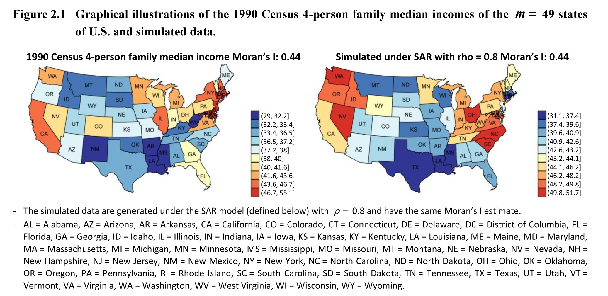
Description of Figure 2.1
Figure illustrating the spatial associations of the 4-person family median incomes of 49 states of the U.S., including the District of Columbia, from the 1990 Census (on the left) and from simulated data (on the right). The legends at the right of each figure indicate the color coding by median income bracket scaled by $1,000. The two figures demonstrate the existence of spatial dependence in the 1990 Census 4-person family median incomes.
To address this issue, we
propose to use spatially correlated random effects. Let
be the adjacency matrix which plays an
important role in capturing spatial dependency. In particular, if the and small areas are connected via geographical
boundary or through other mechanisms (for example, air traffic), and otherwise. Also, for The off-diagonal entries, need not be binary; they can take other
positive values, such as the “length” of the geographical border or volumes of
air traffic between the two areas. Since the adjacency matrix is symmetric, its eigenvalues are real. We
denote the largest eigenvalue of by such that Since is non-null and we get as a result that Let be the sum of the row of and
Assuming that diagonal elements of are positive, i.e., all small areas have at
least 1 neighboring area, we define Since is a row stochastic matrix, all of its
eigenvalues are between -1 and 1, with at least one of them is 1. Consequently,
Moreover, and have the same set of eigenvalues, and the
latter matrix is symmetric. So all the eigenvalues of are real, and will be negative. We consider four alternative
spatial dependencies associated with random effects, which are represented by
the following positive definite precision matrices (excluding the scale
parameter
where is the spatial dependence parameter that
represents the strength of spatial dependence (Hodges, 2019, Chapter 5.2)
and is defined as Since the eigenvalues of are between 0 (the smallest eigenvalue) and (the largest eigenvalue, the matrix is nonnegative definite. Each precision matrix
is guaranteed to be positive definite as long as is in the range specified in the respective
definition.
The adjacency matrix of the simultaneous autoregressive (SAR) model
(Whittle, 1954) is
row-normalized so that can vary from -1 to 1 while preserving the
positive definiteness (Banerjee,
Carlin and Gelfand, 2003,
Chapter 4.4). The model (2.5) is a simple version of conditional
autoregressive (CAR) model (Rao and
Molina, 2015, Chapter 9.6.2), where diagonal entries of the
precision matrix are all equal to one. Even though the diagonal elements of a
precision matrix are all equal, the diagonal elements of the inverse may not be
all equal, leading to heteroscedasticity of random effects. We call this model
the simple conditional autoregressive (SCAR) model. The model (2.6) is widely
used conditional autoregressive model (CAR; Banerjee et al., 2003; Besag and Kooperberg, 1995; You and Zhou,
2011), where diagonal entries of the precision matrix are the number of
neighborhoods of the corresponding area. The upper limit of is and in the case of the model with is referred to as the intrinsic autoregressive
(IAR) model (Banerjee et al.,
2003, Chapter 4.3). The model (2.7) is a conditional autoregressive model, which we call
Leroux’s
conditional autoregressive (LCAR), whose precision matrix is given by
the convex combination of and This model has been considered by Leroux, Lei
and Breslow (2000); MacNab (2003); You
and Zhou (2011), where the diagonal element of is the number of neighborhoods of the small area, and the off-diagonal element is -1 if the and the small areas are connected and 0 otherwise.
The conditional autoregressive
models, SCAR, CAR, and LCAR, assume that depends only on neighboring small area means.
In other words, is correlated with only through the means of surrounding areas.
On the contrary, the SAR model assumes that is dependent on all other concurrently, but has stronger (weaker) correlations for
neighboring (remote) areas. The independent FH model can be viewed as a special
case of the SAR, SCAR, or LCAR model with For notational convenience, we include the
independent FH model as part of our model by taking its precision matrix although it is free from
We consider the following HB spatial models
incorporating the five spatial dependencies defined in (2.4)-(2.7):
where is the model scale parameter, and are suitable functions of and and are the lower and upper bounds of under the model. We avoid the term “model error variance”
for as diagonal entries of vary across small areas and are not
necessarily all one.
2.2 Estimation of population means of non-sampled
small areas
In this section, we consider the
case when, in the survey, there are several non-sampled small areas that have
no direct estimates. In many applications, limited resources frequently
preclude the inclusion of many subpopulations in the sample, resulting in
non-sampled small areas. In this section, we consider the case when, in the
survey, there are several non-sampled small areas that have no direct
estimates. In many applications, limited resources frequently preclude the
inclusion of many subpopulations in the sample, resulting in non-sampled small
areas. Non-sampled small areas are sometimes referred to as misaligned areas (Trevisani and Gelfand, 2013) when
they arise from domain misalignment between the direct estimate and auxiliary
variables. For any of these non-sampled areas, the prediction of its mean from
any non-spatial model is only based on its synthetic estimator. We propose to
exploit spatial dependencies in predicting area means of non-sampled small
areas. The predictions of the proposed models are obtained by modifying its
synthetic estimator, using the vector of regression residuals, with more
emphasis on the regression residuals of the neighboring areas.
Without loss of generality, let
there be non-sampled small areas and be the direct estimates of the sampled small areas. Based on the direct
estimates of sampled areas, we consider the following HB
models:
where and which is the subvector of corresponding to the sampled areas.
2.3 Propriety of the posterior distributions
In this section, we establish
propriety of the posterior distributions of spatial small area models given in
(2.8)-(2.10) and (2.11)-(2.13). Let
be the indicator function taking the value 1
when its argument is true and 0 otherwise. We first provide general conditions
for the posterior propriety of the proposed models.
Theorem 1. For all the HB spatial models
given in (2.8)-(2.10) and (2.11)-(2.13), the posterior probability density
functions are proper if the following conditions hold for some positive
constant
- (a)
- (b)
- (c)
where for (2.8)-(2.10), and for (2.11)-(2.13).
If
is a proper pdf, then (a) holds true
automatically, and (b) is satisfied if The condition is obvious since at least observations are needed to estimate components of when no substantive information about it is
available. Also, any bounded function of satisfies in Theorem 1 as their supports are all
bounded. In particular, under the popular family of noninformative priors
the posterior pdfs are proper under the following
conditions.
Corollary 1. For any of the HB spatial
models given in (2.8)-(2.9) and (2.11)-(2.12) with the prior in (2.14), the
posterior pdf is proper as long as and
For the uniform prior
with (which
will be used in this paper), the propriety of the posterior distributions for
models (2.8)-(2.9) are guaranteed as long as the number of small areas is
greater than For the
models incorporating non-sampled areas given in (2.11)-(2.12), the second
condition of Corollary 1.1 becomes and
thus, the posterior pdfs are proper as long as the number of non-sampled areas
is fewer than or at
least areas
have sample.
