
Multilevel time series modelling of antenatal care coverage in Bangladesh at disaggregated administrative levels
Section 6. Results
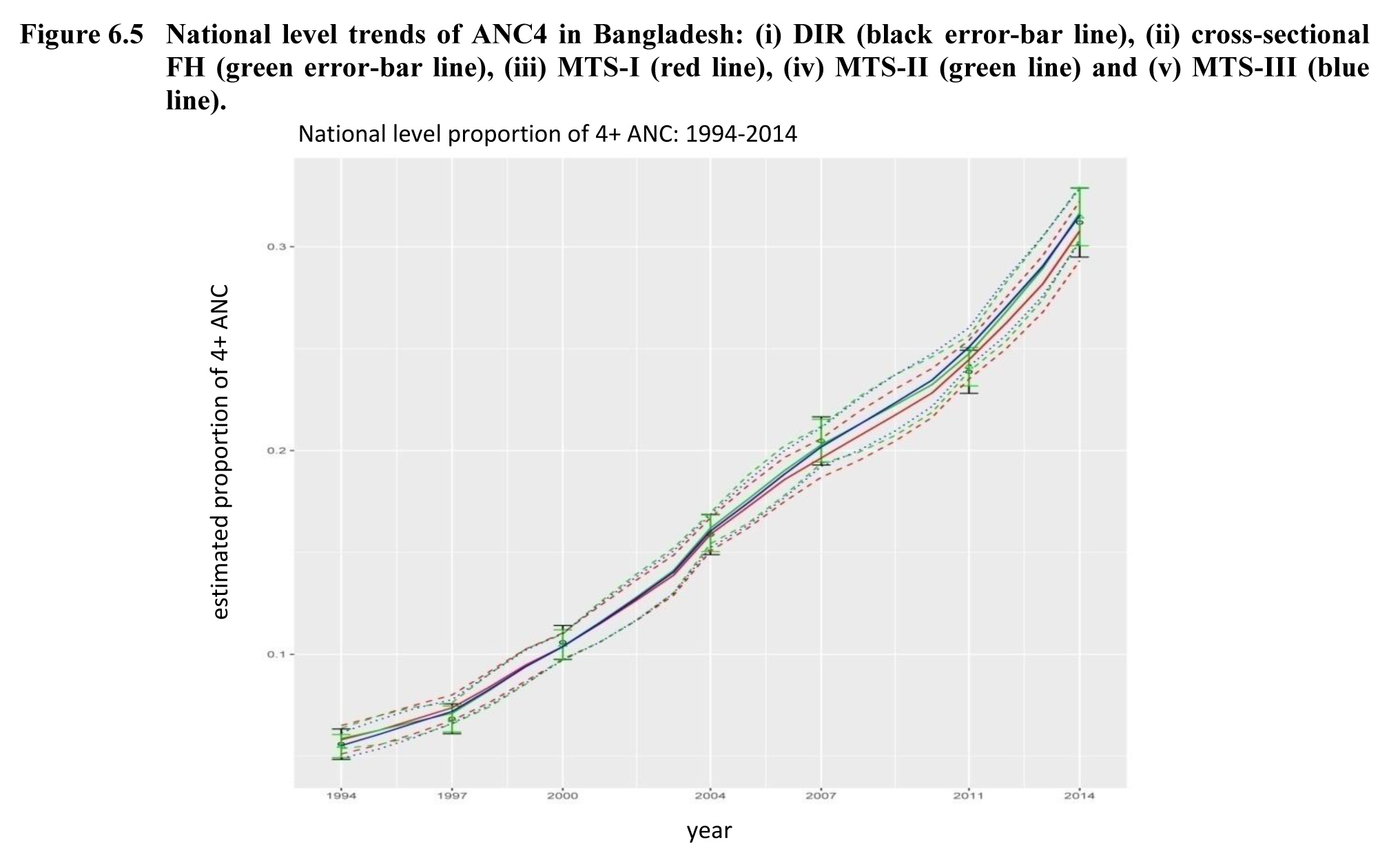
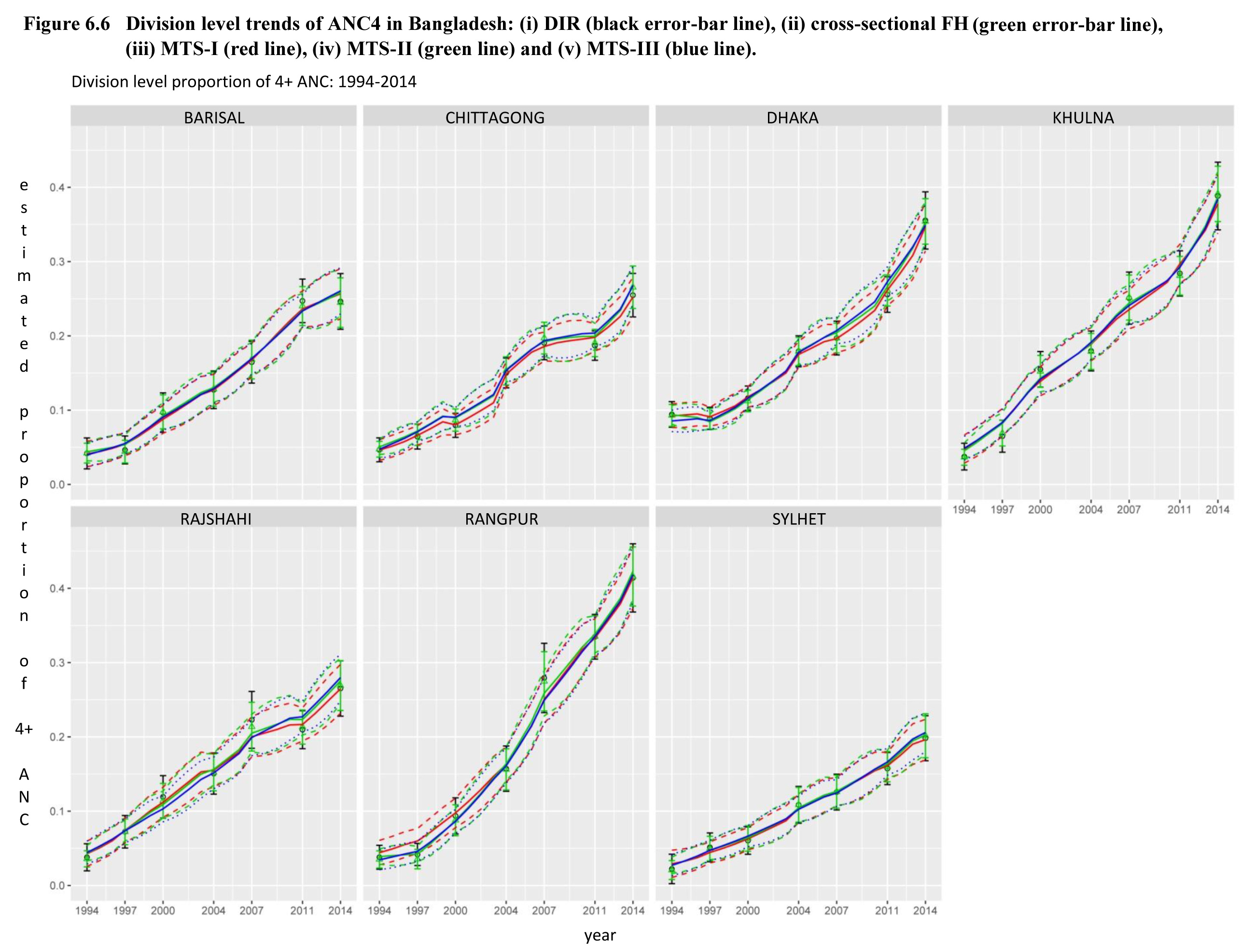
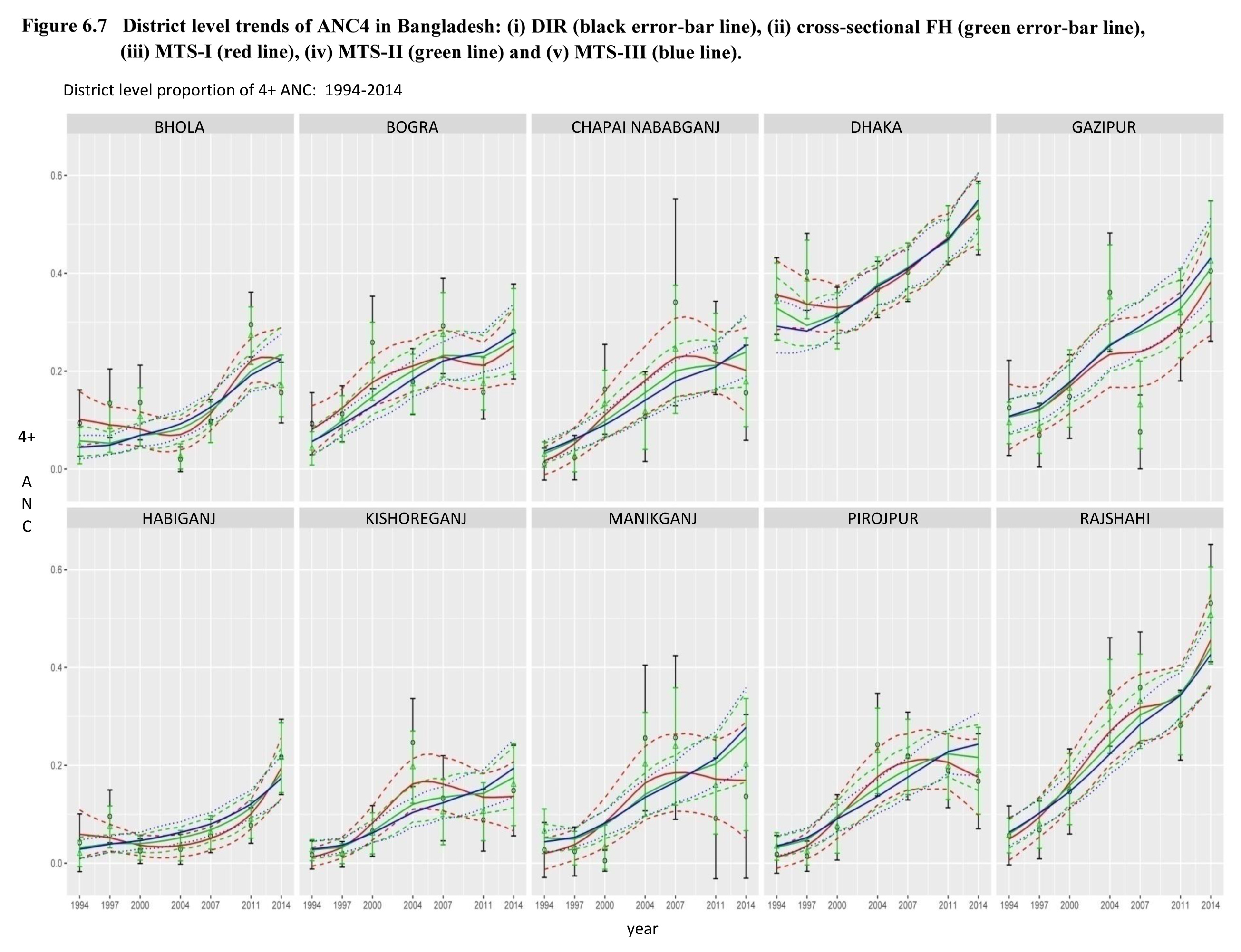
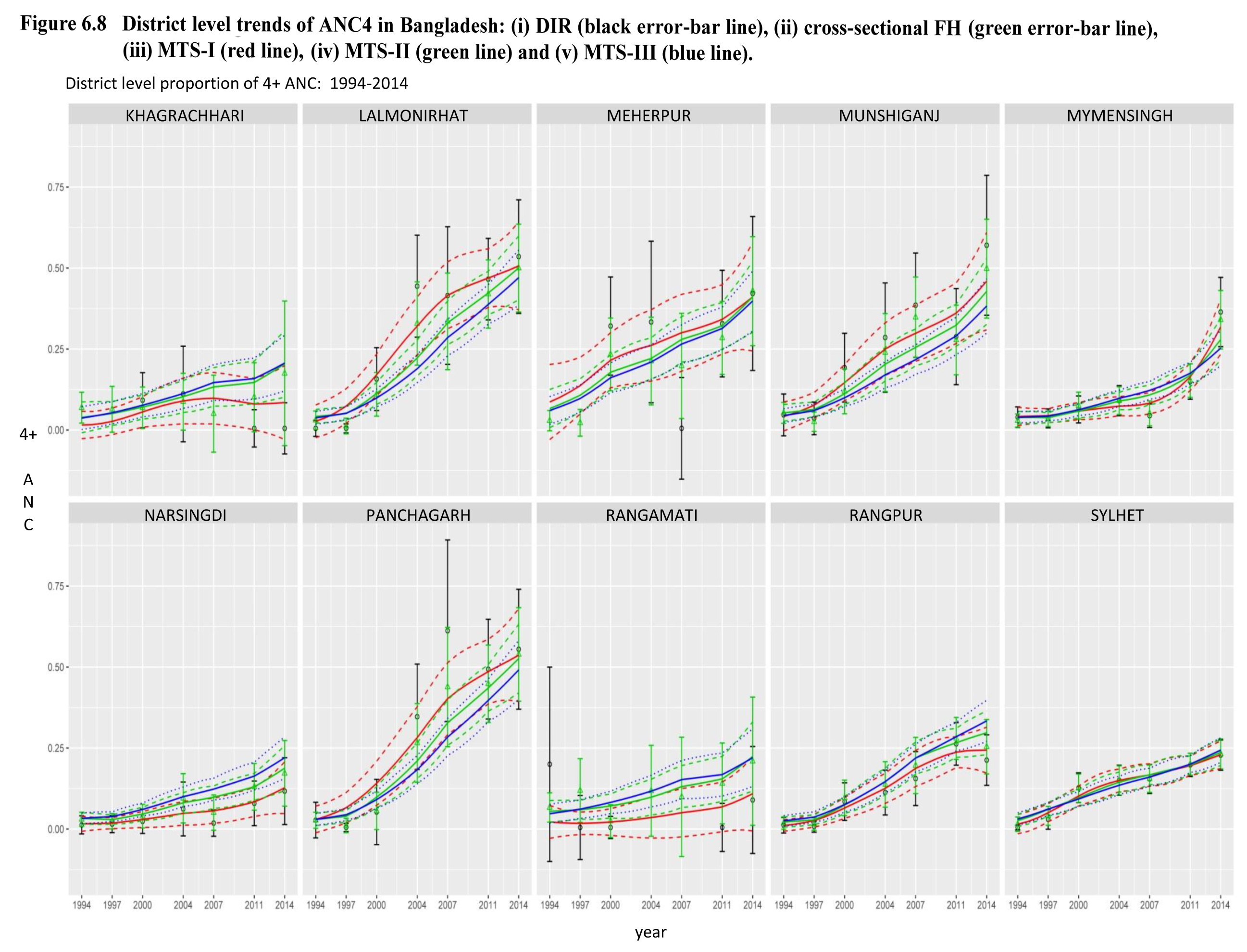
The trends of ANC0 and ANC4 shown in the figures consist of five types of estimates with their approximate 95% confidence intervals: (i) weighted direct estimates (DIR) at the surveyed year (black error-bar line), (ii) cross-sectional FH estimates at the surveyed year (green error-bar line), (iii) estimates based on MTS-I model (red line), (iv) estimates based on MTS-II (green line) and (v) estimates based on MTS-III model (blue line).
6.1 ANC0
The national level trends of ANC0 are shown in Figure 6.1. The figure shows that the DIR and cross-sectional FH estimates are very similar at the survey years with approximately equal 95% CI. This can be expected for figures at the national level, since the gain in precision obtained with a small area prediction model with respect to a direct estimator becomes smaller as the sample size increases. During the initial period 1994-2000, the national level trend based on the MTS-I model follows the DIR and cross-sectional FH estimates, while the trends based on MTS-II and MTS-III models are slightly higher. For the period 2004-2010, the trend based on MTS-I model is slightly higher than the trends based on MTS-II and MTS-III models. The differences are, however, very small.
The trends at division level, shown in Figure 6.2, indicate that the trends under MTS-I are very similar to those based on MTS-II and MTS-III models with some small exceptions in Dhaka, Khulna and Rajshahi divisions. The differences in Dhaka and Khulna division may cause most of the differences in the national level trends.
The trends based on the MTS-II and MTS-III models are almost identical at national and division levels. This is supported by the estimated variance components of the division-level smooth-trend random component under the developed two models about 0.020) given in Table 6.1. However, there are more substantial differences in the trends under MTS-II and MTS-III at the district level, see Figures 6.3 and 6.4. See Das, van den Brakel, Boonstra and Haslett (2021) for plots for all districts. The trends based on the MTS-III model are smoother than those based on the MTS-II model, which is a result of the smaller values of the estimated variance component under MTS-III (see Table 6.1).
| Model | ||||||
|---|---|---|---|---|---|---|
| MTS-I | 0.083 (0.013) | 0.054 (0.007) | 0.168 (0.171) | 0.068 (0.032) | 0.019 (0.003) | 0.024 (0.002) |
| MTS-II | 0.069 (0.012) | 0.033 (0.004) | 0.254 (0.180) | 0.071 (0.028) | 0.020 (0.003) | 0.013 (0.002) |
| MTS-III | 0.062 (0.013) | 0.027 (0.013) | 0.227 (0.201) | 0.067 (0.030) | 0.020 (0.003) | 0.009 (0.001) |
The trends at the district level have a tendency to follow the pattern of their respective division level trend shown in Figure 6.2. This is particularly the case for domains with a relatively small number of observations such as districts Bandarban, Khagrachnari and Rangamati in Figure 6.3 that belong to Chittagong division in Figure 6.2. To reduce this tendency, an MTS model was developed by removing smooth trend component at division level in Table 5.1. This, however, resulted in highly smooth unrealistic trends at the national and divisional levels. In a similar way, to examine the need for a spatial component, MTS models were developed with and without considering the spatial component ( in Table 5.1). It is observed that the spatial component makes the estimates more plausible for those districts with small or zero sample sizes. See for example the trends of Bandarban and Rangamati districts of Chittagong division.
The MTS-I model shows upward trends for some districts during the period of 1994-2000. These developments are unplausible from a subject matter point of view and are nicely corrected by the MTS-II and MTS-III models that use the FH estimates as input series. See for example Noakhali, Bandarban, Rangamati, Narayanganj, Rajbari, and Narail districts in Figure 6.3. Some districts have volatile trends according to the DIR estimates and MTS-I model during the whole period mainly due to variation in the sample size. See for example, Bandarban, Bhola, Khagrachhari, Kishoreganj and Rangamati in Figure 6.3, Chapai Nababganj, Feni, Jhalokati, Joypurhat, and Pabna districts in Figure 6.4. From a subject matter point of view a smooth decreasing trend for ANC0 coverage is expected. In particular the turning points that are visible in several districts arround 2007 and 2011 are not expected. The trends based on the MTS-II and MTS-III models ignore most of these volatilities and show reasonable smooth trends for these districts and are therefore more realistic compared to MTS-I. Nevertheless, the fits of all three models are compatible with the observed data. MTS-II appears to be a nice compromise between models I and III.
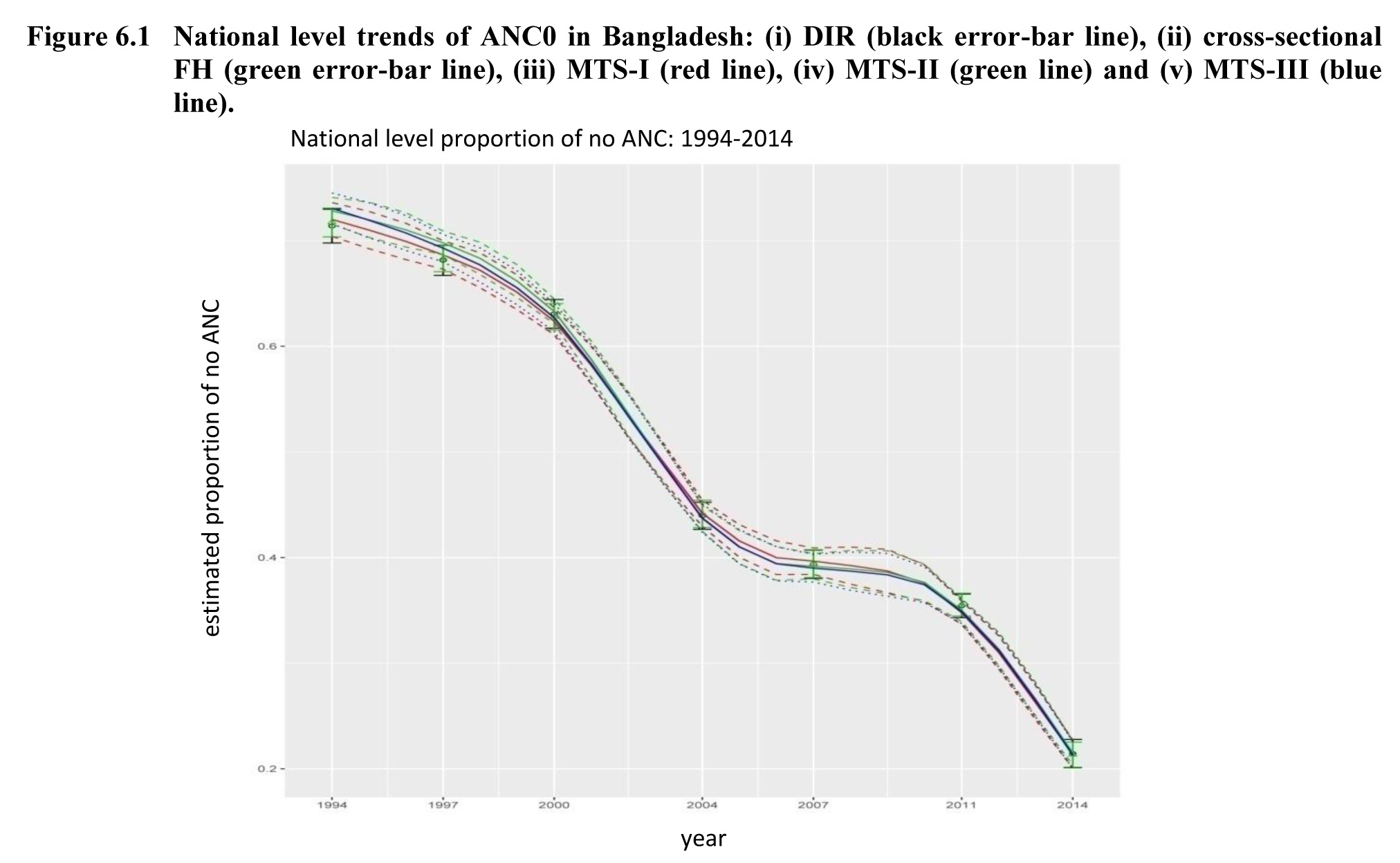
Description of Figure 6.1
Figure presenting the estimated proportions trends of no antenatal care (ANC0) at the national level in Bangladesh (on y-axis) by year (on x-axis), from 1994 to 2014. On the graph, we find the following five models: (i) DIR (black error-bar line); (ii) cross-sectional FH (green error-bar line); (iii) MTS-I (red line); (iv) MTS-II (green line); and (v) MTS-III (blue line). The figure shows that the DIR and cross-sectional FH estimates are very similar at the survey years with approximately equal 95% CI. During the initial period 1994-2000, the national level trend based on the MTS-I model follows the DIR and cross-sectional FH estimates, while the trends based on MTS-II and MTS-III models are slightly higher. For the period 2004-2010, the trend based on MTS-I model is slightly higher than the trends based on MTS-II and MTS-III models. The differences are, however, very small.
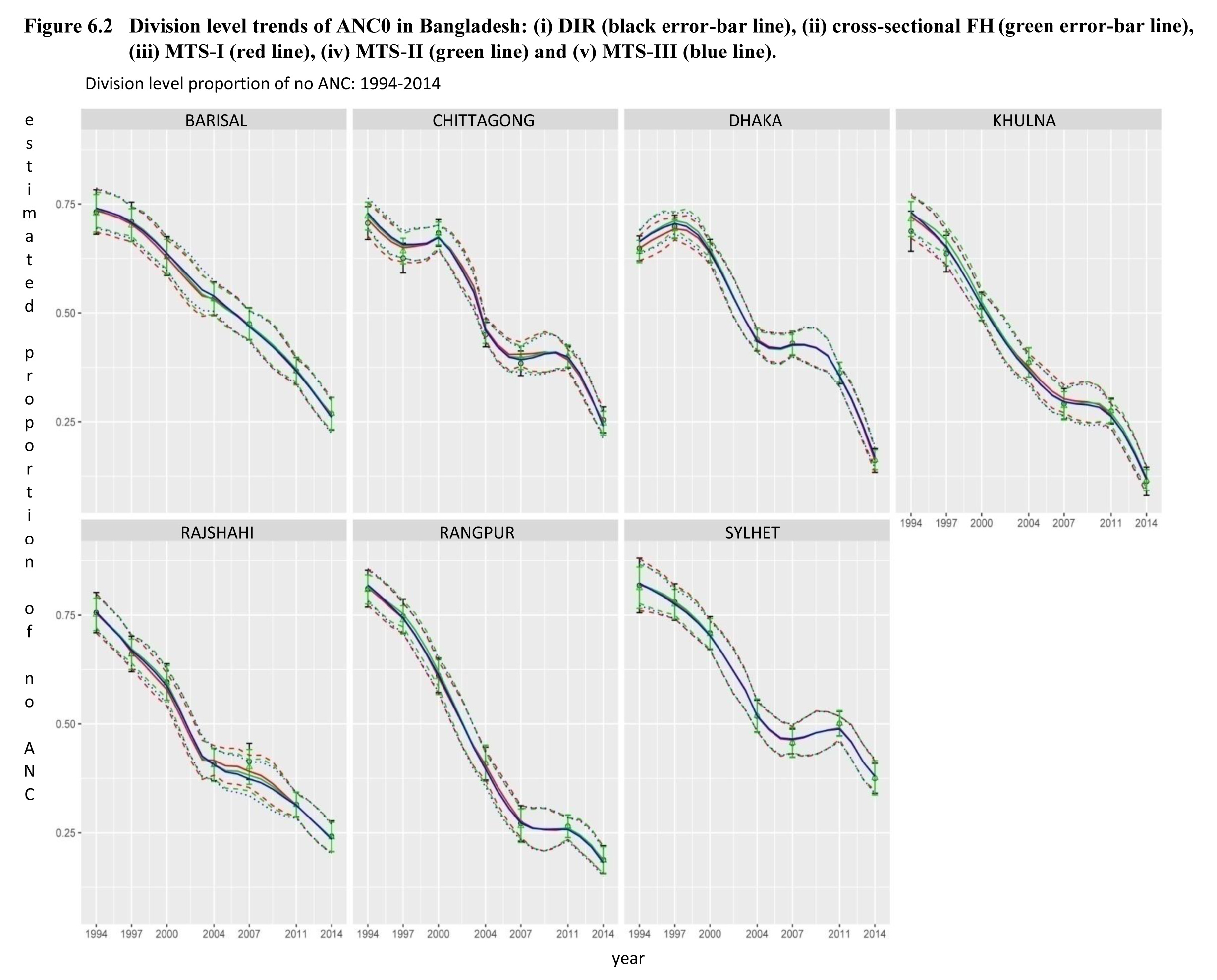
Description of Figure 6.2
Figure presenting the estimated proportions trends of no antenatal care (ANC0) at the division level in Bangladesh (on y-axis) by year (on x-axis), from 1994 to 2014. Each graph represents a division. On the graphs, we find the following five models: (i) DIR (black error-bar line); (ii) cross-sectional FH (green error-bar line); (iii) MTS-I (red line); (iv) MTS-II (green line); and (v) MTS-III (blue line). The trends under MTS-I are very similar to those based on MTS-II and MTS-III models with some small exceptions in Dhaka, Khulna and Rajshahi divisions. The differences in Dhaka and Khulna division may cause most of the differences in the national level trends. The trends based on the MTS-II and MTS-III models are almost identical at national and division levels.
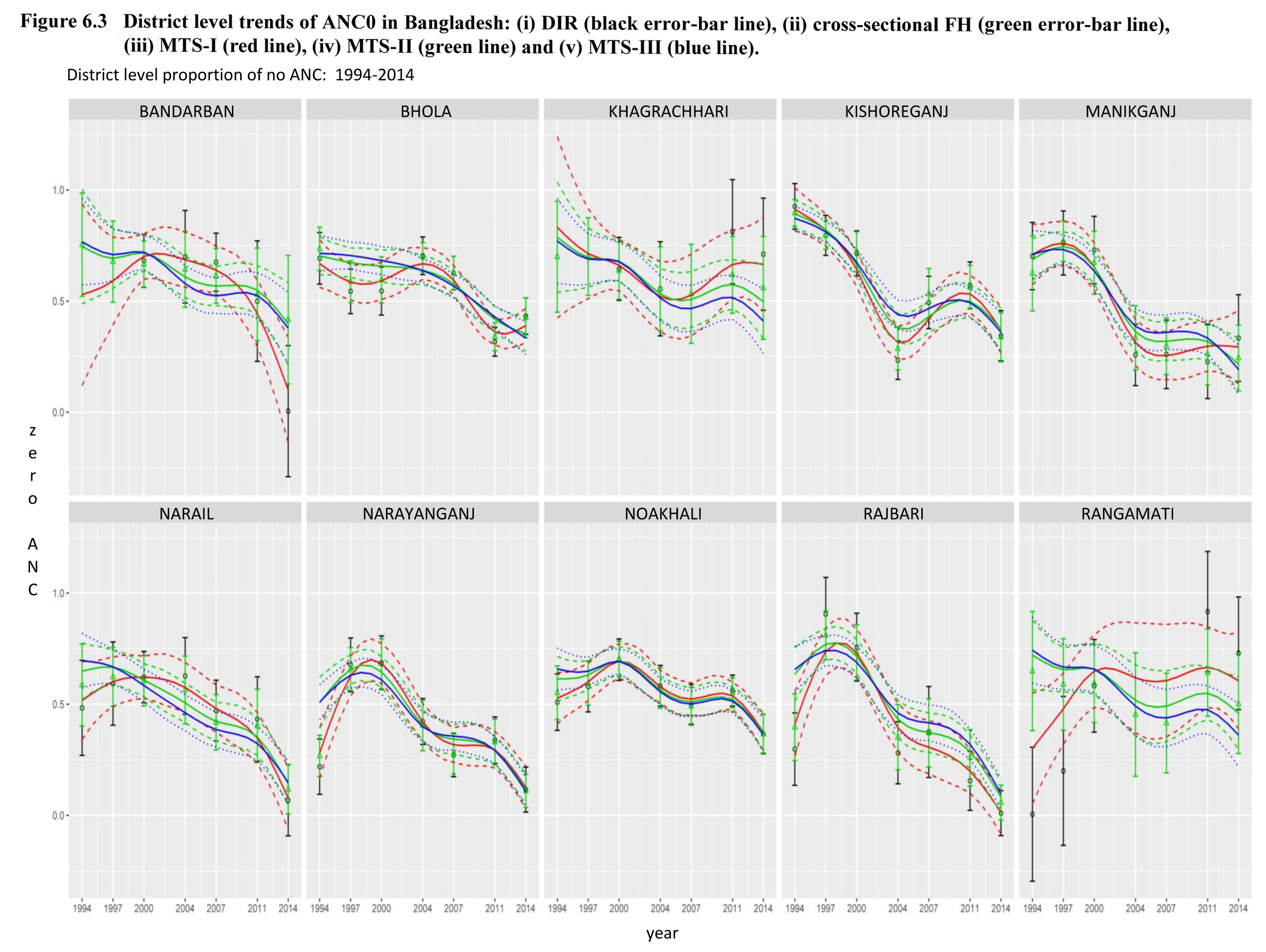
Description of Figure 6.3
Figure presenting the estimated proportions trends of no antenatal care (ANC0) at the district level in Bangladesh (on y-axis) by year (on x-axis), from 1994 to 2014. Each graph represents a district. On the graphs, we find the following five models: (i) DIR (black error-bar line); (ii) cross-sectional FH (green error-bar line); (iii) MTS-I (red line); (iv) MTS-II (green line); and (v) MTS-III (blue line). There are more substantial differences in the trends under MTS-II and MTS-III at the district level. The trends based on the MTS-III model are smoother than those based on the MTS-II model. The trends at the district level have a tendency to follow the pattern of their respective division level trend shown in Figure 6.2. This is particularly the case for domains with a relatively small number of observations such as districts Bandarban, Khagrachnari and Rangamati that belong to Chittagong division in Figure 6.2. In most cases models MTS-II and MTS-III behave similarly. However, model MTS-III, which accounts for correlation among the cross-sectional FH estimates, slightly under estimates the trend in some districts (such as Khagrachari, Rangamati, and Shirajganj districts) compared to the cross-sectional FH estimates.
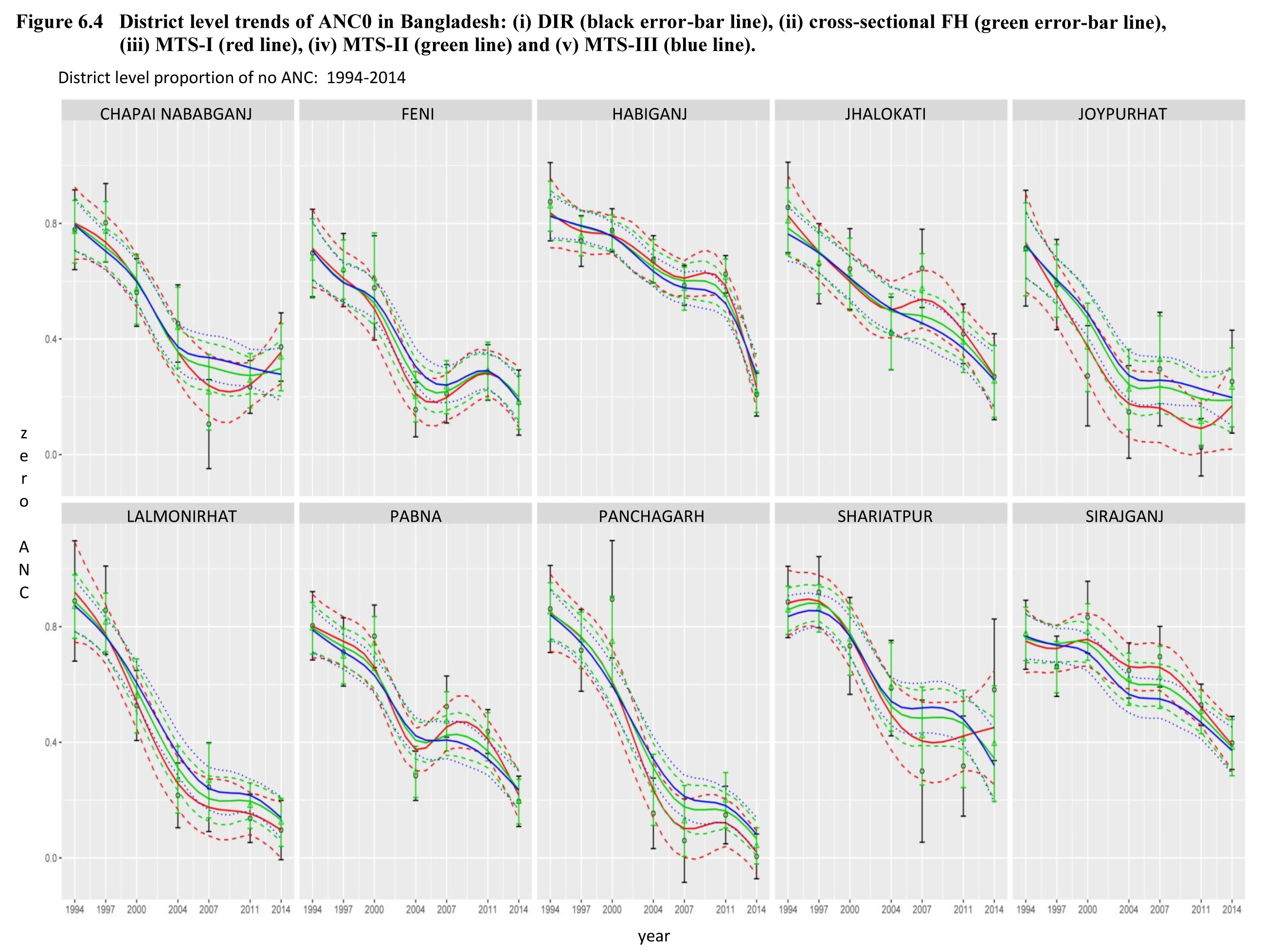
Description of Figure 6.4
Figure presenting the estimated proportions trends of no antenatal care (ANC0) at the district level in Bangladesh (on y-axis) by year (on x-axis), from 1994 to 2014. Each graph represents a district. Figure 6.4 is the continuation of Figure 6.3. On the graphs, we find the following five models: (i) DIR (black error-bar line); (ii) cross-sectional FH (green error-bar line); (iii) MTS-I (red line); (iv) MTS-II (green line); and (v) MTS-III (blue line). There are more substantial differences in the trends under MTS-II and MTS-III at the district level. The trends based on the MTS-III model are smoother than those based on the MTS-II model. The trends at the district level have a tendency to follow the pattern of their respective division level trend shown in Figure 6.2. In most cases models MTS-II and MTS-III behave similarly. However, model MTS-III, which accounts for correlation among the cross-sectional FH estimates, overestimates ANC0 for some districts (such as Chapai Nababganj, Lalmonirhat and Shariatpur districts) compared to the cross-sectional FH estimates.
In most cases models MTS-II and MTS-III behave similarly. However, model MTS-III, which accounts for correlation among the cross-sectional FH estimates, overestimates ANC0 for some districts (such as Chapai Nababganj, Lalmonirhat and Shariatpur districts in Figure 6.4) and also slightly underestimate the trend in some districts (such as Khagrachari, Rangamati, and Shirajganj districts in Figure 6.3) compared to the cross-sectional FH estimates. Again MTS-II seeks a compromise between smooth trends under MTS-III and more volatile trends under MTS-I in most of the districts and appears to be the preferred model for estimating trends of ANC0.
6.2 ANC4
The national level trend of ANC4 shown in Figure 6.5 shows a linear upward increase from 6% in 1994 to about 31% in 2014. Like ANC0, the DIR and cross-sectional FH estimates of ANC4 are very similar at the survey years with approximately equal 95% CI. Trends estimated from the MTS-I (red line), MTS-II (green line) and MTS-III (blue line) show very similar patterns. Compared to the DIR and cross-sectional FH estimates, the trend of MTS-I is slightly lower in 2007 and 2014. Trends under MTS-II and MTS-III in survey year 2011 are somewhat larger compared to the DIR and cross-sectional FH estimates. The trends at division level are shown in Figure 6.6. The three MTS models give very similar trend estimates. Some differences occur in Chittagong, Dhaka and Rangpur divisions. With MTS-I the trend is slightly higher compared to the DIR and FH estimates for Rangpur division over the 1994-2000 period. For MTS-II and MTS-III, the trend is somewhat higher in Rajshahi division during 2011-2014 period compared to the DIR and FH estimates. All three MTS models show slightly bow-shaped 95% CI bands in between two subsequent survey years, which indicates slightly higher uncertainty during the non-survey years compared to the survey years.
Description of Figure 6.5
Figure presenting the estimated proportions trends of at least four antenatal cares (ANC4) at the national level in Bangladesh (on y-axis) by year (on x-axis), from 1994 to 2014. On the graph, we find the following five models: (i) DIR (black error-bar line); (ii) cross-sectional FH (green error-bar line); (iii) MTS-I (red line); (iv) MTS-II (green line); and (v) MTS-III (blue line). The DIR and cross-sectional FH estimates of ANC4 are very similar at the survey years with approximately equal 95% CI. Trends estimated from the MTS-I, MTS-II and MTS-III show very similar patterns. Compared to the DIR and cross-sectional FH estimates, the trend of MTS-I is slightly lower in 2007 and 2014. Trends under MTS-II and MTS-III in survey year 2011 are somewhat larger compared to the DIR and cross-sectional FH estimates.
Description of Figure 6.6
Figure presenting the estimated proportions trends of at least four antenatal cares (ANC4) at the division level in Bangladesh (on y-axis) by year (on x-axis), from 1994 to 2014. Each graph represents a division. On the graphs, we find the following five models: (i) DIR (black error-bar line); (ii) cross-sectional FH (green error-bar line); (iii) MTS-I (red line); (iv) MTS-II (green line); and (v) MTS-III (blue line). The three MTS models give very similar trend estimates. Some differences occur in Chittagong, Dhaka and Rangpur divisions. With MTS-I the trend is slightly higher compared to the DIR and FH estimates for Rangpur division over the 1994-2000 period. For MTS-II and MTS-III, the trend is somewhat higher in Rajshahi division during 2011-2014 period compared to the DIR and FH estimates. All three MTS models show slightly bow-shaped 95% CI bands in between two subsequent survey years, which indicates slightly higher uncertainty during the non-survey years compared to the survey years.
Although the trends based on MTS-II and MTS-III are almost identical at national and division levels, the estimated variance components of both model differ considerably as follows from Table 6.2. These differences lead to substantial differences in the trend estimates at the district level for MTS-II and MTS-III. Plots for some of the districts are provided in Figures 6.7 and 6.8. See Das, van den Brakel, Boonstra and Haslett (2021) for plots of all districts. Similar to ANC0, the trends of ANC4 under MTS-III are smoother than those under MTS-II. The smaller variance components of MTS-III also result in narrower confidence bands compared to MTS-II.
| Model | ||||||
|---|---|---|---|---|---|---|
| MTS-I | 0.060 (0.010) | 0.033 (0.005) | 0.428 (0.178) | 0.047 (0.026) | 0.012 (0.004) | 0.009 (0.001) |
| MTS-II | 0.046 (0.007) | 0.022 (0.003) | 0.501 (0.162) | 0.035 (0.018) | 0.016 (0.003) | 0.004 (0.001) |
| MTS-III | 0.038 (0.006) | 0.018 (0.006) | 0.522 (0.165) | 0.027 (0.016) | 0.014 (0.003) | 0.002 (0.001) |
The trend estimates under MTS-I are volatile and show unexpected downward trends for some districts, see for example Bhola and Pirojpur districts of Barisal division, Gazipur, Kishoreganj and Manikganj of Dhaka division, Bogra, Chapai Nababganj and Rajshahi districts of Rajshahi division, and Habiganj district of Sylhet division in Figure 6.7. From a subject matter point of view, such strong movements and turning points are not expected for ANC4 coverage. Therefore it appears that MTS-I follows the DIR estimates too strongly. The trends under MTS-II generally ignore these volatilities and show reasonably smooth trends for these districts. The trends under MTS-III are even smoother for some of these districts, as for example Bogra and Habiganj districts in Figure 6.7, and Mymensingh and Sylhet districts in Figure 6.8.
The main difficulty arises for the three hilly districts of Chittagong division, i.e., Khagrachhari, Rangamati, and Lakshmipur (the first two districts are plotted in Figure 6.8). MTS-I shows very poor trend estimates for ANC4 over the whole period mainly due to the erratic DIR estimates, which are either zero or highly inconsistent in most of the surveys. The cross-sectional FH estimates are more robust and consequently MTS-II and MTS-III show reasonable upward trends for ANC4. It is expected that women residing in urbanized and better socioeconomic areas are supposed to receive more ANC visits compared to those residing in rural and poor socioeconomic areas. MTS-I shows in some districts lower and in other districts higher than expected trend estimates over the whole time period. For example, the trend obtained with MTS-I for Narsingdi in Figure 6.8, which is a highly urbanized district of Dhaka division, is lower than expected. Similarly the trend under MTS-I Munshiganj in Figure 6.8, which is a less urbanized district of Dhaka is higher than expected. Similarly the trend estimates under MTS-I are over the whole period higher than expected in Meherpur district of Khulna division, Lalmonirhat and Panchagarh districts of Rangpur division. The trend estimates under MTS-II and MTS-III seem more plausible because the cross-sectional FH estimates appear to be more realistic than the DIR estimates. Overall, as in the case of ANC0, MTS-II is a good compromise between MTS-I and MTS-III.
Description of Figure 6.7
Figure presenting the estimated proportions trends of at least four antenatal cares (ANC4) at the district level in Bangladesh (on y-axis) by year (on x-axis), from 1994 to 2014. Each graph represents a district. On the graphs, we find the following five models: (i) DIR (black error-bar line); (ii) cross-sectional FH (green error-bar line); (iii) MTS-I (red line); (iv) MTS-II (green line); and (v) MTS-III (blue line). The trend estimates under MTS-I are volatile and show unexpected downward trends for some districts, see for example Bhola and Pirojpur districts of Barisal division, Gazipur, Kishoreganj and Manikganj of Dhaka division, Bogra, Chapai Nababganj and Rajshahi districts of Rajshahi division, and Habiganj district of Sylhet division. Therefore it appears that MTS-I follows the DIR estimates too strongly. The trends under MTS-II generally ignore these volatilities and show reasonably smooth trends for these districts. The trends under MTS-III are even smoother for some of these districts, as for example Bogra and Habiganj districts.
Description of Figure 6.8
Figure presenting the estimated proportions trends of at least four antenatal cares (ANC4) at the district level in Bangladesh (on y-axis) by year (on x-axis), from 1994 to 2014. Each graph represents a district. Figure 6.8 is the continuation of Figure 6.7. On the graphs, we find the following five models: (i) DIR (black error-bar line); (ii) cross-sectional FH (green error-bar line); (iii) MTS-I (red line); (iv) MTS-II (green line); and (v) MTS-III (blue line). The trend estimates under MTS-I are volatile and show unexpected downward trends for some districts, see for example Bhola and Pirojpur districts of Barisal division, Gazipur, Kishoreganj and Manikganj of Dhaka division, Bogra, Chapai Nababganj and Rajshahi districts of Rajshahi division, and Habiganj district of Sylhet division. Therefore it appears that MTS-I follows the DIR estimates too strongly. The trends under MTS-II generally ignore these volatilities and show reasonably smooth trends for these districts. The trends under MTS-III are even smoother for some of these districts, as for example Mymensingh and Sylhet districts. For the three hilly districts of Chittagong division, i.e., Khagrachhari, Rangamati, and Lakshmipur (the first two districts are plotted in Figure 6.8), MTS-I shows very poor trend estimates for ANC4 over the whole period mainly due to the erratic DIR estimates, which are either zero or highly inconsistent in most of the surveys. The cross-sectional FH estimates are more robust and consequently MTS-II and MTS-III show reasonable upward trends for ANC4. Overall, MTS-II is a good compromise between MTS-I and MTS-III.
- Date modified: