Maximum entropy classification for record linkage
Section 6. Simulation study

6.1   Set-up

To explore the practical feasibility of the unsupervised MEC algorithm for record linkage, we conduct a simulation study based on the data sets listed in Table 6.1, which are disseminated by ESSnet-DI (McLeod, Heasman and Forbes, 2011) and freely available online. Each record in a data set has associated synthetic key variables, which may be distorted by missing values and typos when they are created, in ways that imitate real-life errors (McLeod et al., 2011).


Table 6.1
Data set description (size in parentheses)
Table summary
This table displays the results of Data set description (size in parentheses). The information is grouped by Data set (appearing as row headers), Description (appearing as column headers).
Data set Description
Census (25,343) A fictional data set to represent some observations from a decennial Census.
CIS (24,613) Fictional observations from Customer Information System, combined administrative data from the tax and benefit systems.
PRD (24,750) Fictional observations from Patient Register Data of the National Health Service.

We consider the linkage keys forename, surname, sex, and date of birth (DOB). To model the key variables, we divide DOB into 3 key variables (Day, Month, Year). For text variables such as forename and surname, we divide them into 4 key variables by using the Soundex coding algorithm (Copas and Hilton, 1990, page 290), which reduces a name to a code consisting of the leading letter followed by three digits, e.g. Copas MathType@MTEF@5@5@+= feaagKart1ev2aqatCvAUfeBSjuyZL2yd9gzLbvyNv2CaerbuLwBLn hiov2DGi1BTfMBaeXatLxBI9gBaerbd9wDYLwzYbItLDharqqtubsr 4rNCHbGeaGqiFu0Je9sqqrpepC0xbbf9F4rqqrFfpeea0xe9Lq=Jc9 vqaqpepm0xbba9pwe9Q8fs0=yqaqpepae9pg0FirpepeKkFr0xfr=x fr=xb9adbaqaaeGaciGaaiaabeqaamaabaabaaGcbaGaeyyyIOlaaa@37B2@  C120, Hilton MathType@MTEF@5@5@+= feaagKart1ev2aqatCvAUfeBSjuyZL2yd9gzLbvyNv2CaerbuLwBLn hiov2DGi1BTfMBaeXatLxBI9gBaerbd9wDYLwzYbItLDharqqtubsr 4rNCHbGeaGqiFu0Je9sqqrpepC0xbbf9F4rqqrFfpeea0xe9Lq=Jc9 vqaqpepm0xbba9pwe9Q8fs0=yqaqpepae9pg0FirpepeKkFr0xfr=x fr=xb9adbaqaaeGaciGaaiaabeqaamaabaabaaGcbaGaeyyyIOlaaa@37B2@  H435. The twelve key variables for record linkage are presented in Table 6.2.


Table 6.2
Twelve key variables available in the three data sets
Table summary
This table displays the results of Twelve key variables available in the three data sets. The information is grouped by Variable (appearing as row headers), Description and No. of Categories (appearing as column headers).
Variable Description No. of Categories
PERNAME1 1 First letter of forename 26
2 First digit of Soundex code of forename 7
3 Second digit of Soundex code of forename 7
4 Third digit of Soundex code of forename 7
PERNAME2 1 First letter of surname 26
2 First digit of Soundex code of surname 7
3 Second digit of Soundex code of surname 7
4 Third digit of Soundex code of surname 7
SEX Male/Female 2
DOB DAY Day of birth 31
MON Month of birth 12
YEAR Year of birth (1910 ~ MathType@MTEF@5@5@+= feaagKart1ev2aaatCvAUfeBSjuyZL2yd9gzLbvyNv2CaerbuLwBLn hiov2DGi1BTfMBaeXatLxBI9gBaerbd9wDYLwzYbItLDharqqtubsr 4rNCHbGeaGqk0Jf9crFfpeea0xh9v8qqW7rqqrFfpeea0xe9Lq=Jc9 vqaqpepm0xbba9pwe9Q8fs0=yqaqpepae9pg0FirpepeKkFr0xfr=x fr=xb9adbaqaaeGaciGaaiaabeqaamaabaabaaGcbaacbaGaa8NFaa aa@3931@ 2012) 103

We set up two scenarios to generate linkage files. We use the unique identification variable (PERSON-ID) for sampling, which are available in all the three data sets. We sample n A =500 MathType@MTEF@5@5@+= feaagKart1ev2aqatCvAUfeBSjuyZL2yd9gzLbvyNv2CaerbuLwBLn hiov2DGi1BTfMBaeXatLxBI9gBaerbd9wDYLwzYbItLDharqqtubsr 4rNCHbGeaGqiFu0Je9sqqrpepC0xbbf9F4rqqrFfpeea0xe9Lq=Jc9 vqaqpepm0xbba9pwe9Q8fs0=yqaqpepae9pg0FirpepeKkFr0xfr=x fr=xb9adbaqaaeGaciGaaiaabeqaamaabaabaaGcbaGaamOBamaaBa aaleaacaWGbbaabeaakiaaysW7cqGH9aqpcaaMc8UaaGjbVlaaiwda caaIWaGaaGimaaaa@3FB6@  and n B =1,000 MathType@MTEF@5@5@+= feaagKart1ev2aqatCvAUfeBSjuyZL2yd9gzLbvyNv2CaerbuLwBLn hiov2DGi1BTfMBaeXatLxBI9gBaerbd9wDYLwzYbItLDharqqtubsr 4rNCHbGeaGqiFu0Je9sqqrpepC0xbbf9F4rqqrFfpeea0xe9Lq=Jc9 vqaqpepm0xbba9pwe9Q8fs0=yqaqpepae9pg0FirpepeKkFr0xfr=x fr=xb9adbaqaaeGaciGaaiaabeqaamaabaabaaGcbaGaamOBamaaBa aaleaacaWGcbaabeaakiaaysW7cqGH9aqpcaaMc8UaaGjbVlaabgda caqGSaGaaeimaiaabcdacaqGWaaaaa@4100@  individuals from PRD and CIS, respectively. Let p A MathType@MTEF@5@5@+= feaagKart1ev2aqatCvAUfeBSjuyZL2yd9gzLbvyNv2CaerbuLwBLn hiov2DGi1BTfMBaeXatLxBI9gBaerbd9wDYLwzYbItLDharqqtubsr 4rNCHbGeaGqiFu0Je9sqqrpepC0xbbf9F4rqqrFfpeea0xe9Lq=Jc9 vqaqpepm0xbba9pwe9Q8fs0=yqaqpepae9pg0FirpepeKkFr0xfr=x fr=xb9adbaqaaeGaciGaaiaabeqaamaabaabaaGcbaGaamiCamaaBa aaleaacaWGbbaabeaaaaa@37D0@  be the proportion of records in the smaller file (PRD) that are also selected in the larger file (CIS), by which we can vary the degree of overlap, i.e. the set of matched individuals AB, MathType@MTEF@5@5@+= feaagKart1ev2aqatCvAUfeBSjuyZL2yd9gzLbvyNv2CaerbuLwBLn hiov2DGi1BTfMBaeXatLxBI9gBaerbd9wDYLwzYbItLDharqqtubsr 4rNCHbGeaGqiFu0Je9sqqrpepC0xbbf9F4rqqrFfpeea0xe9Lq=Jc9 vqaqpepm0xbba9pwe9Q8fs0=yqaqpepae9pg0FirpepeKkFr0xfr=x fr=xb9adbaqaaeGaciGaaiaabeqaamaabaabaaGcbaGaamyqaiaadk eacaGGSaaaaa@3826@  between A MathType@MTEF@5@5@+= feaagKart1ev2aqatCvAUfeBSjuyZL2yd9gzLbvyNv2CaerbuLwBLn hiov2DGi1BTfMBaeXatLxBI9gBaerbd9wDYLwzYbItLDharqqtubsr 4rNCHbGeaGqiFu0Je9sqqrpepC0xbbf9F4rqqrFfpeea0xe9Lq=Jc9 vqaqpepm0xbba9pwe9Q8fs0=yqaqpepae9pg0FirpepeKkFr0xfr=x fr=xb9adbaqaaeGaciGaaiaabeqaamaabaabaaGcbaGaamyqaaaa@36AF@  and B. MathType@MTEF@5@5@+= feaagKart1ev2aqatCvAUfeBSjuyZL2yd9gzLbvyNv2CaerbuLwBLn hiov2DGi1BTfMBaeXatLxBI9gBaerbd9wDYLwzYbItLDharqqtubsr 4rNCHbGeaGqiFu0Je9sqqrpepC0xbbf9F4rqqrFfpeea0xe9Lq=Jc9 vqaqpepm0xbba9pwe9Q8fs0=yqaqpepae9pg0FirpepeKkFr0xfr=x fr=xb9adbaqaaeGaciGaaiaabeqaamaabaabaaGcbaGaamOqaiaac6 caaaa@3762@  We use p A =0.8,0.5 MathType@MTEF@5@5@+= feaagKart1ev2aqatCvAUfeBSjuyZL2yd9gzLbvyNv2CaerbuLwBLn hiov2DGi1BTfMBaeXatLxBI9gBaerbd9wDYLwzYbItLDharqqtubsr 4rNCHbGeaGqiFu0Je9sqqrpepC0xbbf9F4rqqrFfpeea0xe9Lq=Jc9 vqaqpepm0xbba9pwe9Q8fs0=yqaqpepae9pg0FirpepeKkFr0xfr=x fr=xb9adbaqaaeGaciGaaiaabeqaamaabaabaaGcbaGaamiCamaaBa aaleaacaWGbbaabeaakiaaysW7cqGH9aqpcaaMc8UaaGjbVlaabcda caqGUaGaaeioaiaacYcacaaMc8UaaGPaVlaabcdacaqGUaGaaeynaa aa@4586@  or 0.3 under either scenario.

Scenario-I (Non-informative)

Under this scenario both δ a MathType@MTEF@5@5@+= feaagKart1ev2aqatCvAUfeBSjuyZL2yd9gzLbvyNv2CaerbuLwBLn hiov2DGi1BTfMBaeXatLxBI9gBaerbd9wDYLwzYbItLDharqqtubsr 4rNCHbGeaGqiFu0Je9sqqrpepC0xbbf9F4rqqrFfpeea0xe9Lq=Jc9 vqaqpepm0xbba9pwe9Q8fs0=yqaqpepae9pg0FirpepeKkFr0xfr=x fr=xb9adbaqaaeGaciGaaiaabeqaamaabaabaaGcbaGaeqiTdq2aaS baaSqaaiaadggaaeqaaaaa@38A0@  and δ b MathType@MTEF@5@5@+= feaagKart1ev2aqatCvAUfeBSjuyZL2yd9gzLbvyNv2CaerbuLwBLn hiov2DGi1BTfMBaeXatLxBI9gBaerbd9wDYLwzYbItLDharqqtubsr 4rNCHbGeaGqiFu0Je9sqqrpepC0xbbf9F4rqqrFfpeea0xe9Lq=Jc9 vqaqpepm0xbba9pwe9Q8fs0=yqaqpepae9pg0FirpepeKkFr0xfr=x fr=xb9adbaqaaeGaciGaaiaabeqaamaabaabaaGcbaGaeqiTdq2aaS baaSqaaiaadkgaaeqaaaaa@38A1@  are non-informative for the key-variable distribution. For any given p A , MathType@MTEF@5@5@+= feaagKart1ev2aqatCvAUfeBSjuyZL2yd9gzLbvyNv2CaerbuLwBLn hiov2DGi1BTfMBaeXatLxBI9gBaerbd9wDYLwzYbItLDharqqtubsr 4rNCHbGeaGqiFu0Je9sqqrpepC0xbbf9F4rqqrFfpeea0xe9Lq=Jc9 vqaqpepm0xbba9pwe9Q8fs0=yqaqpepae9pg0FirpepeKkFr0xfr=x fr=xb9adbaqaaeGaciGaaiaabeqaamaabaabaaGcbaGaamiCamaaBa aaleaacaWGbbaabeaakiaacYcaaaa@388A@  we have E( n M )= n A p A MathType@MTEF@5@5@+= feaagKart1ev2aqatCvAUfeBSjuyZL2yd9gzLbvyNv2CaerbuLwBLn hiov2DGi1BTfMBaeXatLxBI9gBaerbd9wDYLwzYbItLDharqqtubsr 4rNCHbGeaGqiFu0Je9sqqrpepC0xbbf9F4rqqrFfpeea0xe9Lq=Jc9 vqaqpepm0xbba9pwe9Q8fs0=yqaqpepae9pg0FirpepeKkFr0xfr=x fr=xb9adbaqaaeGaciGaaiaabeqaamaabaabaaGcbaGaamyraiaayk W7daqadeqaaiaad6gadaWgaaWcbaGaamytaaqabaaakiaawIcacaGL PaaacaaMe8Uaeyypa0JaaGjbVlaad6gadaWgaaWcbaGaamyqaaqaba GccaWGWbWaaSbaaSqaaiaadgeaaeqaaaaa@43B9@  and π= E( n M )/ n 0 , MathType@MTEF@5@5@+= feaagKart1ev2aqatCvAUfeBSjuyZL2yd9gzLbvyNv2CaerbuLwBLn hiov2DGi1BTfMBaeXatLxBI9gBaerbd9wDYLwzYbItLDharqqtubsr 4rNCHbGeaGqiFu0Je9sqqrpepC0xbbf9F4rqqrFfpeea0xe9Lq=Jc9 vqaqpepm0xbba9pwe9Q8fs0=yqaqpepae9pg0FirpepeKkFr0xfr=x fr=xb9adbaqaaeGaciGaaiaabeqaamaabaabaaGcbaGaeqiWdaNaaG jbVlabg2da9iaaysW7daWcgaqaaiaadweacaaMc8+aaeWabeaacaWG UbWaaSbaaSqaaiaad2eaaeqaaaGccaGLOaGaayzkaaGaaGPaVdqaai aaykW7caWGUbWaaSbaaSqaaiaaicdaaeqaaaaakiaacYcaaaa@475F@  where n M MathType@MTEF@5@5@+= feaagKart1ev2aqatCvAUfeBSjuyZL2yd9gzLbvyNv2CaerbuLwBLn hiov2DGi1BTfMBaeXatLxBI9gBaerbd9wDYLwzYbItLDharqqtubsr 4rNCHbGeaGqiFu0Je9sqqrpepC0xbbf9F4rqqrFfpeea0xe9Lq=Jc9 vqaqpepm0xbba9pwe9Q8fs0=yqaqpepae9pg0FirpepeKkFr0xfr=x fr=xb9adbaqaaeGaciGaaiaabeqaamaabaabaaGcbaGaamOBamaaBa aaleaacaWGnbaabeaaaaa@37DA@  is the random number of matched individuals between the simulated files A MathType@MTEF@5@5@+= feaagKart1ev2aqatCvAUfeBSjuyZL2yd9gzLbvyNv2CaerbuLwBLn hiov2DGi1BTfMBaeXatLxBI9gBaerbd9wDYLwzYbItLDharqqtubsr 4rNCHbGeaGqiFu0Je9sqqrpepC0xbbf9F4rqqrFfpeea0xe9Lq=Jc9 vqaqpepm0xbba9pwe9Q8fs0=yqaqpepae9pg0FirpepeKkFr0xfr=x fr=xb9adbaqaaeGaciGaaiaabeqaamaabaabaaGcbaGaamyqaaaa@36AF@  and B. MathType@MTEF@5@5@+= feaagKart1ev2aqatCvAUfeBSjuyZL2yd9gzLbvyNv2CaerbuLwBLn hiov2DGi1BTfMBaeXatLxBI9gBaerbd9wDYLwzYbItLDharqqtubsr 4rNCHbGeaGqiFu0Je9sqqrpepC0xbbf9F4rqqrFfpeea0xe9Lq=Jc9 vqaqpepm0xbba9pwe9Q8fs0=yqaqpepae9pg0FirpepeKkFr0xfr=x fr=xb9adbaqaaeGaciGaaiaabeqaamaabaabaaGcbaGaamOqaiaac6 caaaa@3762@

Scenario-II (Informative)

Under this scenario the key-variable distribution is the same in A, MathType@MTEF@5@5@+= feaagKart1ev2aqatCvAUfeBSjuyZL2yd9gzLbvyNv2CaerbuLwBLn hiov2DGi1BTfMBaeXatLxBI9gBaerbd9wDYLwzYbItLDharqqtubsr 4rNCHbGeaGqiFu0Je9sqqrpepC0xbbf9F4rqqrFfpeea0xe9Lq=Jc9 vqaqpepm0xbba9pwe9Q8fs0=yqaqpepae9pg0FirpepeKkFr0xfr=x fr=xb9adbaqaaeGaciGaaiaabeqaamaabaabaaGcbaGaamyqaiaacY caaaa@375F@  whether or not δ a =1, MathType@MTEF@5@5@+= feaagKart1ev2aqatCvAUfeBSjuyZL2yd9gzLbvyNv2CaerbuLwBLn hiov2DGi1BTfMBaeXatLxBI9gBaerbd9wDYLwzYbItLDharqqtubsr 4rNCHbGeaGqiFu0Je9sqqrpepC0xbbf9F4rqqrFfpeea0xe9Lq=Jc9 vqaqpepm0xbba9pwe9Q8fs0=yqaqpepae9pg0FirpepeKkFr0xfr=x fr=xb9adbaqaaeGaciGaaiaabeqaamaabaabaaGcbaGaeqiTdq2aaS baaSqaaiaadggaaeqaaOGaaGjbVlabg2da9iaaysW7caaIXaGaaiil aaaa@3E35@  but it is different for the records b B 0 , MathType@MTEF@5@5@+= feaagKart1ev2aqatCvAUfeBSjuyZL2yd9gzLbvyNv2CaerbuLwBLn hiov2DGi1BTfMBaeXatLxBI9gBaerbd9wDYLwzYbItLDharqqtubsr 4rNCHbGeaGqiFu0Je9sqqrpepC0xbbf9F4rqqrFfpeea0xe9Lq=Jc9 vqaqpepm0xbba9pwe9Q8fs0=yqaqpepae9pg0FirpepeKkFr0xfr=x fr=xb9adbaqaaeGaciGaaiaabeqaamaabaabaaGcbaGaamOyaiaays W7cqGHiiIZcaaMe8UaamOqamaaBaaaleaacaaIWaaabeaakiaacYca aaa@3DD5@  or δ b =0. MathType@MTEF@5@5@+= feaagKart1ev2aqatCvAUfeBSjuyZL2yd9gzLbvyNv2CaerbuLwBLn hiov2DGi1BTfMBaeXatLxBI9gBaerbd9wDYLwzYbItLDharqqtubsr 4rNCHbGeaGqiFu0Je9sqqrpepC0xbbf9F4rqqrFfpeea0xe9Lq=Jc9 vqaqpepm0xbba9pwe9Q8fs0=yqaqpepae9pg0FirpepeKkFr0xfr=x fr=xb9adbaqaaeGaciGaaiaabeqaamaabaabaaGcbaGaeqiTdq2aaS baaSqaaiaadkgaaeqaaOGaaGjbVlabg2da9iaaysW7caaIWaGaaiOl aaaa@3E37@  Hence, scenario-II is informative. For any given p A , MathType@MTEF@5@5@+= feaagKart1ev2aqatCvAUfeBSjuyZL2yd9gzLbvyNv2CaerbuLwBLn hiov2DGi1BTfMBaeXatLxBI9gBaerbd9wDYLwzYbItLDharqqtubsr 4rNCHbGeaGqiFu0Je9sqqrpepC0xbbf9F4rqqrFfpeea0xe9Lq=Jc9 vqaqpepm0xbba9pwe9Q8fs0=yqaqpepae9pg0FirpepeKkFr0xfr=x fr=xb9adbaqaaeGaciGaaiaabeqaamaabaabaaGcbaGaamiCamaaBa aaleaacaWGbbaabeaakiaacYcaaaa@388A@  we have fixed n M = n A p A MathType@MTEF@5@5@+= feaagKart1ev2aqatCvAUfeBSjuyZL2yd9gzLbvyNv2CaerbuLwBLn hiov2DGi1BTfMBaeXatLxBI9gBaerbd9wDYLwzYbItLDharqqtubsr 4rNCHbGeaGqiFu0Je9sqqrpepC0xbbf9F4rqqrFfpeea0xe9Lq=Jc9 vqaqpepm0xbba9pwe9Q8fs0=yqaqpepae9pg0FirpepeKkFr0xfr=x fr=xb9adbaqaaeGaciGaaiaabeqaamaabaabaaGcbaGaamOBamaaBa aaleaacaWGnbaabeaakiaaysW7cqGH9aqpcaaMe8UaamOBamaaBaaa leaacaWGbbaabeaakiaadchadaWgaaWcbaGaamyqaaqabaaaaa@3FDA@  and π= p A / n B . MathType@MTEF@5@5@+= feaagKart1ev2aqatCvAUfeBSjuyZL2yd9gzLbvyNv2CaerbuLwBLn hiov2DGi1BTfMBaeXatLxBI9gBaerbd9wDYLwzYbItLDharqqtubsr 4rNCHbGeaGqiFu0Je9sqqrpepC0xbbf9F4rqqrFfpeea0xe9Lq=Jc9 vqaqpepm0xbba9pwe9Q8fs0=yqaqpepae9pg0FirpepeKkFr0xfr=x fr=xb9adbaqaaeGaciGaaiaabeqaamaabaabaaGcbaGaeqiWdaNaaG jbVlabg2da9iaaysW7daWcgaqaaiaadchadaWgaaWcbaGaamyqaaqa baGccaaMc8oabaGaaGPaVlaad6gadaWgaaWcbaGaamOqaaqabaaaaO GaaiOlaaaa@4385@

6.2   Results: Estimation

For the unsupervised MEC algorithm given in Section 4.1, one can adopt (4.2) or (5.1) for updating θ k ( t ) . MathType@MTEF@5@5@+= feaagKart1ev2aqatCvAUfeBSjuyZL2yd9gzLbvyNv2CaerbuLwBLn hiov2DGi1BTfMBaeXatLxBI9gBaerbd9wDYLwzYbItLDharqqtubsr 4rNCHbGeaGqiFu0Je9sqqrpepC0xbbf9F4rqqrFfpeea0xe9Lq=Jc9 vqaqpepm0xbba9pwe9Q8fs0=yqaqpepae9pg0FirpepeKkFr0xfr=x fr=xb9adbaqaaeGaciGaaiaabeqaamaabaabaaGcbaGaeqiUde3aa0 baaSqaaiaadUgaaeaadaqadeqaaiaadshaaiaawIcacaGLPaaaaaGc caGGUaaaaa@3BFB@  Moreover, one can use (4.4) for ξ ^ k MathType@MTEF@5@5@+= feaagKart1ev2aqatCvAUfeBSjuyZL2yd9gzLbvyNv2CaerbuLwBLn hiov2DGi1BTfMBaeXatLxBI9gBaerbd9wDYLwzYbItLDharqqtubsr 4rNCHbGeaGqiFu0Je9sqqrpepC0xbbf9F4rqqrFfpeea0xe9Lq=Jc9 vqaqpepm0xbba9pwe9Q8fs0=yqaqpepae9pg0FirpepeKkFr0xfr=x fr=xb9adbaqaaeGaciGaaiaabeqaamaabaabaaGcbaGafqOVdGNbaK aadaWgaaWcbaGaam4Aaaqabaaaaa@38D8@  directly, or (5.3) for updating ξ k ( t ) MathType@MTEF@5@5@+= feaagKart1ev2aqatCvAUfeBSjuyZL2yd9gzLbvyNv2CaerbuLwBLn hiov2DGi1BTfMBaeXatLxBI9gBaerbd9wDYLwzYbItLDharqqtubsr 4rNCHbGeaGqiFu0Je9sqqrpepC0xbbf9F4rqqrFfpeea0xe9Lq=Jc9 vqaqpepm0xbba9pwe9Q8fs0=yqaqpepae9pg0FirpepeKkFr0xfr=x fr=xb9adbaqaaeGaciGaaiaabeqaamaabaabaaGcbaGaeqOVdG3aa0 baaSqaaiaadUgaaeaadaqadeqaaiaadshaaiaawIcacaGLPaaaaaaa aa@3B4C@  iteratively. In particular, choosing (5.1) and (4.4) effectively incorporates the procedure of Winkler (1988) and Jaro (1989) for parameter estimation. Note that the MEC approach still differs to that of Jaro (1989), with respect to the formation of the linked set M ^ . MathType@MTEF@5@5@+= feaagKart1ev2aqatCvAUfeBSjuyZL2yd9gzLbvyNv2CaerbuLwBLn hiov2DGi1BTfMBaeXatLxBI9gBaerbd9wDYLwzYbItLDharqqtubsr 4rNCHbGeaGqiFu0Je9sqqrpepC0xbbf9F4rqqrFfpeea0xe9Lq=Jc9 vqaqpepm0xbba9pwe9Q8fs0=yqaqpepae9pg0FirpepeKkFr0xfr=x fr=xb9adbaqaaeGaciGaaiaabeqaamaabaabaaGcbaGabmytayaaja GaaiOlaaaa@377D@

Table 6.3 compares the performance of the unsupervised MEC algorithm, using different formulae for θ k ( t ) MathType@MTEF@5@5@+= feaagKart1ev2aqatCvAUfeBSjuyZL2yd9gzLbvyNv2CaerbuLwBLn hiov2DGi1BTfMBaeXatLxBI9gBaerbd9wDYLwzYbItLDharqqtubsr 4rNCHbGeaGqiFu0Je9sqqrpepC0xbbf9F4rqqrFfpeea0xe9Lq=Jc9 vqaqpepm0xbba9pwe9Q8fs0=yqaqpepae9pg0FirpepeKkFr0xfr=x fr=xb9adbaqaaeGaciGaaiaabeqaamaabaabaaGcbaGaeqiUde3aa0 baaSqaaiaadUgaaeaadaqadeqaaiaadshaaiaawIcacaGLPaaaaaaa aa@3B3F@  and ξ k ( t ) , MathType@MTEF@5@5@+= feaagKart1ev2aqatCvAUfeBSjuyZL2yd9gzLbvyNv2CaerbuLwBLn hiov2DGi1BTfMBaeXatLxBI9gBaerbd9wDYLwzYbItLDharqqtubsr 4rNCHbGeaGqiFu0Je9sqqrpepC0xbbf9F4rqqrFfpeea0xe9Lq=Jc9 vqaqpepm0xbba9pwe9Q8fs0=yqaqpepae9pg0FirpepeKkFr0xfr=x fr=xb9adbaqaaeGaciGaaiaabeqaamaabaabaaGcbaGaeqOVdG3aa0 baaSqaaiaadUgaaeaadaqadeqaaiaadshaaiaawIcacaGLPaaaaaGc caGGSaaaaa@3C06@  where the size of M ^ MathType@MTEF@5@5@+= feaagKart1ev2aqatCvAUfeBSjuyZL2yd9gzLbvyNv2CaerbuLwBLn hiov2DGi1BTfMBaeXatLxBI9gBaerbd9wDYLwzYbItLDharqqtubsr 4rNCHbGeaGqiFu0Je9sqqrpepC0xbbf9F4rqqrFfpeea0xe9Lq=Jc9 vqaqpepm0xbba9pwe9Q8fs0=yqaqpepae9pg0FirpepeKkFr0xfr=x fr=xb9adbaqaaeGaciGaaiaabeqaamaabaabaaGcbaGabmytayaaja aaaa@36CB@  is equal to the corresponding estimate n ^ M . MathType@MTEF@5@5@+= feaagKart1ev2aqatCvAUfeBSjuyZL2yd9gzLbvyNv2CaerbuLwBLn hiov2DGi1BTfMBaeXatLxBI9gBaerbd9wDYLwzYbItLDharqqtubsr 4rNCHbGeaGqiFu0Je9sqqrpepC0xbbf9F4rqqrFfpeea0xe9Lq=Jc9 vqaqpepm0xbba9pwe9Q8fs0=yqaqpepae9pg0FirpepeKkFr0xfr=x fr=xb9adbaqaaeGaciGaaiaabeqaamaabaabaaGcbaGabmOBayaaja WaaSbaaSqaaiaad2eaaeqaaOGaaiOlaaaa@38A6@  In addition, we include θ ^ k = n M ( 1;k )/ n M MathType@MTEF@5@5@+= feaagKart1ev2aqatCvAUfeBSjuyZL2yd9gzLbvyNv2CaerbuLwBLn hiov2DGi1BTfMBaeXatLxBI9gBaerbd9wDYLwzYbItLDharqqtubsr 4rNCHbGeaGqiFu0Je9sqqrpepC0xbbf9F4rqqrFfpeea0xe9Lq=Jc9 vqaqpepm0xbba9pwe9Q8fs0=yqaqpepae9pg0FirpepeKkFr0xfr=x fr=xb9adbaqaaeGaciGaaiaabeqaamaabaabaaGcbaGafqiUdeNbaK aadaWgaaWcbaGaam4AaaqabaGccaaMe8Uaeyypa0JaaGjbVpaalyaa baGaamOBamaaBaaaleaacaWGnbaabeaakmaabmqabaGaaGymaiaaiU dacaaMe8Uaam4AaaGaayjkaiaawMcaaiaaykW7aeaacaaMc8UaamOB amaaBaaaleaacaWGnbaabeaaaaaaaa@4994@  estimated directly from the matched pairs in M, MathType@MTEF@5@5@+= feaagKart1ev2aqatCvAUfeBSjuyZL2yd9gzLbvyNv2CaerbuLwBLn hiov2DGi1BTfMBaeXatLxBI9gBaerbd9wDYLwzYbItLDharqqtubsr 4rNCHbGeaGqiFu0Je9sqqrpepC0xbbf9F4rqqrFfpeea0xe9Lq=Jc9 vqaqpepm0xbba9pwe9Q8fs0=yqaqpepae9pg0FirpepeKkFr0xfr=x fr=xb9adbaqaaeGaciGaaiaabeqaamaabaabaaGcbaGaamytaiaacY caaaa@376B@  as if M MathType@MTEF@5@5@+= feaagKart1ev2aqatCvAUfeBSjuyZL2yd9gzLbvyNv2CaerbuLwBLn hiov2DGi1BTfMBaeXatLxBI9gBaerbd9wDYLwzYbItLDharqqtubsr 4rNCHbGeaGqiFu0Je9sqqrpepC0xbbf9F4rqqrFfpeea0xe9Lq=Jc9 vqaqpepm0xbba9pwe9Q8fs0=yqaqpepae9pg0FirpepeKkFr0xfr=x fr=xb9adbaqaaeGaciGaaiaabeqaamaabaabaaGcbaGaamytaaaa@36BB@  were available for supervised learning, together with (4.4) for ξ ^ k . MathType@MTEF@5@5@+= feaagKart1ev2aqatCvAUfeBSjuyZL2yd9gzLbvyNv2CaerbuLwBLn hiov2DGi1BTfMBaeXatLxBI9gBaerbd9wDYLwzYbItLDharqqtubsr 4rNCHbGeaGqiFu0Je9sqqrpepC0xbbf9F4rqqrFfpeea0xe9Lq=Jc9 vqaqpepm0xbba9pwe9Q8fs0=yqaqpepae9pg0FirpepeKkFr0xfr=x fr=xb9adbaqaaeGaciGaaiaabeqaamaabaabaaGcbaGafqOVdGNbaK aadaWgaaWcbaGaam4AaaqabaGccaGGUaaaaa@3994@  The true parameters and error rates are given in addition to their estimates.


Table 6.3
Parameters and averages of their estimates, averages of error rates and their estimates, over 200 simulations. Median of estimate of n M MathType@MTEF@5@5@+= feaagKart1ev2aqatCvAUfeBSjuyZL2yd9gzLbvyNv2CaerbuLwBLn hiov2DGi1BTfMBaeXatLxBI9gBaerbd9wDYLwzYbItLDharqqtubsr 4rNCHbGeaGqipu0Je9sqqrpepC0xbbf9F4rqqrFfpeea0xe9Lq=Jc9 vqaqpepm0xbba9pwe9Q8fs0=yqaqpepae9pg0FirpepeKkFr0xfr=x fr=xb9adbeqabeWacmGabiqabeqabmqabeabbaGcbaGaamOBamaaBa aaleaacaWGnbaabeaaaaa@37D4@ given as n ˜ M MathType@MTEF@5@5@+= feaagKart1ev2aqatCvAUfeBSjuyZL2yd9gzLbvyNv2CaerbuLwBLn hiov2DGi1BTfMBaeXatLxBI9gBaerbd9wDYLwzYbItLDharqqtubsr 4rNCHbGeaGqipu0Je9sqqrpepC0xbbf9F4rqqrFfpeea0xe9Lq=Jc9 vqaqpepm0xbba9pwe9Q8fs0=yqaqpepae9pg0FirpepeKkFr0xfr=x fr=xb9adbeqabeWacmGabiqabeqabmqabeabbaGcbaGabmOBayaaia WaaSbaaSqaaiaad2eaaeqaaaaa@37E3@
Table summary
This table displays the results of Parameters and averages of their estimates Scenario I and Scenario II (appearing as column headers).
Scenario I Scenario II
Parameter Formulae Estimation Parameter Formulae Estimation
π MathType@MTEF@5@5@+= feaagKart1ev2aqatCvAUfeBSjuyZL2yd9gzLbvyNv2CaerbuLwBLn hiov2DGi1BTfMBaeXatLxBI9gBaerbd9wDYLwzYbItLDharqqtubsr 4rNCHbGeaGWj0Jf9crFfpeea0xh9v8qqW7rqqrFfpeea0xe9Lq=Jc9 vqaqpepm0xbba9pwe9Q8fs0=yqaqpepae9pg0FirpepeKkFr0xfr=x fr=xb9adbeqabeWacmGabiqabeqabmqabeabbaGcbaGaeqiWdahaaa@39EF@ E( n M ) MathType@MTEF@5@5@+= feaagKart1ev2aqatCvAUfeBSjuyZL2yd9gzLbvyNv2CaerbuLwBLn hiov2DGi1BTfMBaeXatLxBI9gBaerbd9wDYLwzYbItLDharqqtubsr 4rNCHbGeaGWj0Jf9crFfpeea0xh9v8qqW7rqqrFfpeea0xe9Lq=Jc9 vqaqpepm0xbba9pwe9Q8fs0=yqaqpepae9pg0FirpepeKkFr0xfr=x fr=xb9adbeqabeWacmGabiqabeqabmqabeabbaGcbaGaamyraiaayk W7daqadeqaaiaad6gadaWgaaWcbaGaamytaaqabaaakiaawIcacaGL Paaaaaa@3E0C@ θ k ( t ) MathType@MTEF@5@5@+= feaagKart1ev2aqatCvAUfeBSjuyZL2yd9gzLbvyNv2CaerbuLwBLn hiov2DGi1BTfMBaeXatLxBI9gBaerbd9wDYLwzYbItLDharqqtubsr 4rNCHbGeaGWj0Jf9crFfpeea0xh9v8qqW7rqqrFfpeea0xe9Lq=Jc9 vqaqpepm0xbba9pwe9Q8fs0=yqaqpepae9pg0FirpepeKkFr0xfr=x fr=xb9adbeqabeWacmGabiqabeqabmqabeabbaGcbaGaeqiUde3aa0 baaSqaaiaadUgaaeaacaaMc8+aaeWabeaacaWG0baacaGLOaGaayzk aaaaaaaa@3F13@ ξ k ( t ) MathType@MTEF@5@5@+= feaagKart1ev2aqatCvAUfeBSjuyZL2yd9gzLbvyNv2CaerbuLwBLn hiov2DGi1BTfMBaeXatLxBI9gBaerbd9wDYLwzYbItLDharqqtubsr 4rNCHbGeaGWj0Jf9crFfpeea0xh9v8qqW7rqqrFfpeea0xe9Lq=Jc9 vqaqpepm0xbba9pwe9Q8fs0=yqaqpepae9pg0FirpepeKkFr0xfr=x fr=xb9adbeqabeWacmGabiqabeqabmqabeabbaGcbaGaeqOVdG3aa0 baaSqaaiaadUgaaeaacaaMc8+aaeWabeaacaWG0baacaGLOaGaayzk aaaaaaaa@3F20@ π ^ MathType@MTEF@5@5@+= feaagKart1ev2aqatCvAUfeBSjuyZL2yd9gzLbvyNv2CaerbuLwBLn hiov2DGi1BTfMBaeXatLxBI9gBaerbd9wDYLwzYbItLDharqqtubsr 4rNCHbGeaGWj0Jf9crFfpeea0xh9v8qqW7rqqrFfpeea0xe9Lq=Jc9 vqaqpepm0xbba9pwe9Q8fs0=yqaqpepae9pg0FirpepeKkFr0xfr=x fr=xb9adbeqabeWacmGabiqabeqabmqabeabbaGcbaGafqiWdaNbaK aaaaa@39FF@ n ^ M MathType@MTEF@5@5@+= feaagKart1ev2aqatCvAUfeBSjuyZL2yd9gzLbvyNv2CaerbuLwBLn hiov2DGi1BTfMBaeXatLxBI9gBaerbd9wDYLwzYbItLDharqqtubsr 4rNCHbGeaGWj0Jf9crFfpeea0xh9v8qqW7rqqrFfpeea0xe9Lq=Jc9 vqaqpepm0xbba9pwe9Q8fs0=yqaqpepae9pg0FirpepeKkFr0xfr=x fr=xb9adbeqabeWacmGabiqabeqabmqabeabbaGcbaGabmOBayaaja WaaSbaaSqaaiaad2eaaeqaaaaa@3A33@ n ˜ M MathType@MTEF@5@5@+= feaagKart1ev2aqatCvAUfeBSjuyZL2yd9gzLbvyNv2CaerbuLwBLn hiov2DGi1BTfMBaeXatLxBI9gBaerbd9wDYLwzYbItLDharqqtubsr 4rNCHbGeaGWj0Jf9crFfpeea0xh9v8qqW7rqqrFfpeea0xe9Lq=Jc9 vqaqpepm0xbba9pwe9Q8fs0=yqaqpepae9pg0FirpepeKkFr0xfr=x fr=xb9adbeqabeWacmGabiqabeqabmqabeabbaGcbaGabmOBayaaia WaaSbaaSqaaiaad2eaaeqaaaaa@3A32@ FLR MMR FLR ^ MathType@MTEF@5@5@+= feaagKart1ev2aqatCvAUfeBSjuyZL2yd9gzLbvyNv2CaerbuLwBLn hiov2DGi1BTfMBaeXatLxBI9gBaerbd9wDYLwzYbItLDharqqtubsr 4rNCHbGeaGqiVu0Je9sqqrpepC0xbbL8F4rqqrFfpeea0xe9Lq=Jc9 vqaqpepm0xbba9pwe9Q8fs0=yqaqpepae9pg0FirpepeKkFr0xfr=x fr=xb9adbaqaaeGaciGaaiaabeqaamaabaabaaGcbaWaaecaaeaaqa aaaaaaaaWdbiaaboeacaqGqbGaae4taaWdaiaawkWaamaaBaaaleaa peGaamyAaaWdaeqaaaaa@3A8C@ MMR ^ MathType@MTEF@5@5@+= feaagKart1ev2aqatCvAUfeBSjuyZL2yd9gzLbvyNv2CaerbuLwBLn hiov2DGi1BTfMBaeXatLxBI9gBaerbd9wDYLwzYbItLDharqqtubsr 4rNCHbGeaGqiVu0Je9sqqrpepC0xbbL8F4rqqrFfpeea0xe9Lq=Jc9 vqaqpepm0xbba9pwe9Q8fs0=yqaqpepae9pg0FirpepeKkFr0xfr=x fr=xb9adbaqaaeGaciGaaiaabeqaamaabaabaaGcbaWaaecaaeaaqa aaaaaaaaWdbiaaboeacaqGqbGaae4taaWdaiaawkWaamaaBaaaleaa peGaamyAaaWdaeqaaaaa@3A8C@ π MathType@MTEF@5@5@+= feaagKart1ev2aqatCvAUfeBSjuyZL2yd9gzLbvyNv2CaerbuLwBLn hiov2DGi1BTfMBaeXatLxBI9gBaerbd9wDYLwzYbItLDharqqtubsr 4rNCHbGeaGWj0Jf9crFfpeea0xh9v8qqW7rqqrFfpeea0xe9Lq=Jc9 vqaqpepm0xbba9pwe9Q8fs0=yqaqpepae9pg0FirpepeKkFr0xfr=x fr=xb9adbeqabeWacmGabiqabeqabmqabeabbaGcbaGaeqiWdahaaa@39EF@ n M MathType@MTEF@5@5@+= feaagKart1ev2aqatCvAUfeBSjuyZL2yd9gzLbvyNv2CaerbuLwBLn hiov2DGi1BTfMBaeXatLxBI9gBaerbd9wDYLwzYbItLDharqqtubsr 4rNCHbGeaGWj0Jf9crFfpeea0xh9v8qqW7rqqrFfpeea0xe9Lq=Jc9 vqaqpepm0xbba9pwe9Q8fs0=yqaqpepae9pg0FirpepeKkFr0xfr=x fr=xb9adbeqabeWacmGabiqabeqabmqabeabbaGcbaGaamOBamaaBa aaleaacaWGnbaabeaaaaa@3A23@ θ k ( t ) MathType@MTEF@5@5@+= feaagKart1ev2aqatCvAUfeBSjuyZL2yd9gzLbvyNv2CaerbuLwBLn hiov2DGi1BTfMBaeXatLxBI9gBaerbd9wDYLwzYbItLDharqqtubsr 4rNCHbGeaGWj0Jf9crFfpeea0xh9v8qqW7rqqrFfpeea0xe9Lq=Jc9 vqaqpepm0xbba9pwe9Q8fs0=yqaqpepae9pg0FirpepeKkFr0xfr=x fr=xb9adbeqabeWacmGabiqabeqabmqabeabbaGcbaGaeqiUde3aa0 baaSqaaiaadUgaaeaacaaMc8+aaeWabeaacaWG0baacaGLOaGaayzk aaaaaaaa@3F13@ ξ k ( t ) MathType@MTEF@5@5@+= feaagKart1ev2aqatCvAUfeBSjuyZL2yd9gzLbvyNv2CaerbuLwBLn hiov2DGi1BTfMBaeXatLxBI9gBaerbd9wDYLwzYbItLDharqqtubsr 4rNCHbGeaGWj0Jf9crFfpeea0xh9v8qqW7rqqrFfpeea0xe9Lq=Jc9 vqaqpepm0xbba9pwe9Q8fs0=yqaqpepae9pg0FirpepeKkFr0xfr=x fr=xb9adbeqabeWacmGabiqabeqabmqabeabbaGcbaGaeqOVdG3aa0 baaSqaaiaadUgaaeaacaaMc8+aaeWabeaacaWG0baacaGLOaGaayzk aaaaaaaa@3F20@ π ^ MathType@MTEF@5@5@+= feaagKart1ev2aqatCvAUfeBSjuyZL2yd9gzLbvyNv2CaerbuLwBLn hiov2DGi1BTfMBaeXatLxBI9gBaerbd9wDYLwzYbItLDharqqtubsr 4rNCHbGeaGWj0Jf9crFfpeea0xh9v8qqW7rqqrFfpeea0xe9Lq=Jc9 vqaqpepm0xbba9pwe9Q8fs0=yqaqpepae9pg0FirpepeKkFr0xfr=x fr=xb9adbeqabeWacmGabiqabeqabmqabeabbaGcbaGafqiWdaNbaK aaaaa@39FF@ n ^ M MathType@MTEF@5@5@+= feaagKart1ev2aqatCvAUfeBSjuyZL2yd9gzLbvyNv2CaerbuLwBLn hiov2DGi1BTfMBaeXatLxBI9gBaerbd9wDYLwzYbItLDharqqtubsr 4rNCHbGeaGWj0Jf9crFfpeea0xh9v8qqW7rqqrFfpeea0xe9Lq=Jc9 vqaqpepm0xbba9pwe9Q8fs0=yqaqpepae9pg0FirpepeKkFr0xfr=x fr=xb9adbeqabeWacmGabiqabeqabmqabeabbaGcbaGabmOBayaaja WaaSbaaSqaaiaad2eaaeqaaaaa@3A33@ n ˜ M MathType@MTEF@5@5@+= feaagKart1ev2aqatCvAUfeBSjuyZL2yd9gzLbvyNv2CaerbuLwBLn hiov2DGi1BTfMBaeXatLxBI9gBaerbd9wDYLwzYbItLDharqqtubsr 4rNCHbGeaGWj0Jf9crFfpeea0xh9v8qqW7rqqrFfpeea0xe9Lq=Jc9 vqaqpepm0xbba9pwe9Q8fs0=yqaqpepae9pg0FirpepeKkFr0xfr=x fr=xb9adbeqabeWacmGabiqabeqabmqabeabbaGcbaGabmOBayaaia WaaSbaaSqaaiaad2eaaeqaaaaa@3A32@ FLR MMR FLR ^ MathType@MTEF@5@5@+= feaagKart1ev2aqatCvAUfeBSjuyZL2yd9gzLbvyNv2CaerbuLwBLn hiov2DGi1BTfMBaeXatLxBI9gBaerbd9wDYLwzYbItLDharqqtubsr 4rNCHbGeaGqiVu0Je9sqqrpepC0xbbL8F4rqqrFfpeea0xe9Lq=Jc9 vqaqpepm0xbba9pwe9Q8fs0=yqaqpepae9pg0FirpepeKkFr0xfr=x fr=xb9adbaqaaeGaciGaaiaabeqaamaabaabaaGcbaWaaecaaeaaqa aaaaaaaaWdbiaaboeacaqGqbGaae4taaWdaiaawkWaamaaBaaaleaa peGaamyAaaWdaeqaaaaa@3A8C@ MMR ^ MathType@MTEF@5@5@+= feaagKart1ev2aqatCvAUfeBSjuyZL2yd9gzLbvyNv2CaerbuLwBLn hiov2DGi1BTfMBaeXatLxBI9gBaerbd9wDYLwzYbItLDharqqtubsr 4rNCHbGeaGqiVu0Je9sqqrpepC0xbbL8F4rqqrFfpeea0xe9Lq=Jc9 vqaqpepm0xbba9pwe9Q8fs0=yqaqpepae9pg0FirpepeKkFr0xfr=x fr=xb9adbaqaaeGaciGaaiaabeqaamaabaabaaGcbaWaaecaaeaaqa aaaaaaaaWdbiaaboeacaqGqbGaae4taaWdaiaawkWaamaaBaaaleaa peGaamyAaaWdaeqaaaaa@3A8C@
0.0008 400 θ ^ k MathType@MTEF@5@5@+= feaagKart1ev2aqatCvAUfeBSjuyZL2yd9gzLbvyNv2CaerbuLwBLn hiov2DGi1BTfMBaeXatLxBI9gBaerbd9wDYLwzYbItLDharqqtubsr 4rNCHbGeaGWj0Jf9crFfpeea0xh9v8qqW7rqqrFfpeea0xe9Lq=Jc9 vqaqpepm0xbba9pwe9Q8fs0=yqaqpepae9pg0FirpepeKkFr0xfr=x fr=xb9adbaqaaeGaciGaaiaabeqaamaabaabaaGcbaGafqiUdeNbaK aadaWgaaWcbaGaam4Aaaqabaaaaa@3B0A@ (4.4) 0.00080 400.0 397 0.0264 0.0266 0.0357 0.0357 0.0008 400 θ ^ k MathType@MTEF@5@5@+= feaagKart1ev2aqatCvAUfeBSjuyZL2yd9gzLbvyNv2CaerbuLwBLn hiov2DGi1BTfMBaeXatLxBI9gBaerbd9wDYLwzYbItLDharqqtubsr 4rNCHbGeaGWj0Jf9crFfpeea0xh9v8qqW7rqqrFfpeea0xe9Lq=Jc9 vqaqpepm0xbba9pwe9Q8fs0=yqaqpepae9pg0FirpepeKkFr0xfr=x fr=xb9adbaqaaeGaciGaaiaabeqaamaabaabaaGcbaGafqiUdeNbaK aadaWgaaWcbaGaam4Aaaqabaaaaa@3B0A@ (4.4) 0.00080 398.3 400 0.0230 0.0273 0.0326 0.0326
(4.2) (5.3) 0.00082 407.9 405 0.0425 0.0257 0.0509 0.0509 (4.2) (5.3) 0.00080 401.4 401 0.0305 0.0277 0.0403 0.0403
(4.2) (4.4) 0.00083 414.7 407 0.0549 0.0244 0.0620 0.0620 (4.2) (4.4) 0.00081 405.2 404 0.0379 0.0262 0.0467 0.0467
(5.1) (4.4) 0.00081 406.0 405 0.0399 0.0269 0.0503 0.0503 (5.1) (4.4) 0.00080 401.4 401 0.0316 0.0286 0.0438 0.0438
0.0005 250 θ ^ k MathType@MTEF@5@5@+= feaagKart1ev2aqatCvAUfeBSjuyZL2yd9gzLbvyNv2CaerbuLwBLn hiov2DGi1BTfMBaeXatLxBI9gBaerbd9wDYLwzYbItLDharqqtubsr 4rNCHbGeaGWj0Jf9crFfpeea0xh9v8qqW7rqqrFfpeea0xe9Lq=Jc9 vqaqpepm0xbba9pwe9Q8fs0=yqaqpepae9pg0FirpepeKkFr0xfr=x fr=xb9adbaqaaeGaciGaaiaabeqaamaabaabaaGcbaGafqiUdeNbaK aadaWgaaWcbaGaam4Aaaqabaaaaa@3B0A@ (4.4) 0.00050 251.6 249 0.0340 0.0301 0.0370 0.0370 0.0005 250 θ ^ k MathType@MTEF@5@5@+= feaagKart1ev2aqatCvAUfeBSjuyZL2yd9gzLbvyNv2CaerbuLwBLn hiov2DGi1BTfMBaeXatLxBI9gBaerbd9wDYLwzYbItLDharqqtubsr 4rNCHbGeaGWj0Jf9crFfpeea0xh9v8qqW7rqqrFfpeea0xe9Lq=Jc9 vqaqpepm0xbba9pwe9Q8fs0=yqaqpepae9pg0FirpepeKkFr0xfr=x fr=xb9adbaqaaeGaciGaaiaabeqaamaabaabaaGcbaGafqiUdeNbaK aadaWgaaWcbaGaam4Aaaqabaaaaa@3B0A@ (4.4) 0.00050 249.6 250 0.0284 0.0302 0.0334 0.0334
(4.2) (5.3) 0.00052 258.3 255 0.0559 0.0296 0.0533 0.0533 (4.2) (5.3) 0.00050 251.8 251 0.0383 0.0320 0.0410 0.0410
(4.2) (4.4) 0.00053 266.9 256.5 0.0742 0.0277 0.0680 0.0680 (4.2) (4.4) 0.00052 257.7 253 0.0513 0.0295 0.0516 0.0516
(5.1) (4.4) 0.00052 261.7 259 0.0676 0.0305 0.0636 0.0636 (5.1) (4.4) 0.00051 255.4 253.5 0.0510 0.0336 0.0520 0.0520
0.0003 150 θ ^ k MathType@MTEF@5@5@+= feaagKart1ev2aqatCvAUfeBSjuyZL2yd9gzLbvyNv2CaerbuLwBLn hiov2DGi1BTfMBaeXatLxBI9gBaerbd9wDYLwzYbItLDharqqtubsr 4rNCHbGeaGWj0Jf9crFfpeea0xh9v8qqW7rqqrFfpeea0xe9Lq=Jc9 vqaqpepm0xbba9pwe9Q8fs0=yqaqpepae9pg0FirpepeKkFr0xfr=x fr=xb9adbaqaaeGaciGaaiaabeqaamaabaabaaGcbaGafqiUdeNbaK aadaWgaaWcbaGaam4Aaaqabaaaaa@3B0A@ (4.4) 0.00030 152.3 151 0.0439 0.0356 0.0381 0.0381 0.0003 150 θ ^ k MathType@MTEF@5@5@+= feaagKart1ev2aqatCvAUfeBSjuyZL2yd9gzLbvyNv2CaerbuLwBLn hiov2DGi1BTfMBaeXatLxBI9gBaerbd9wDYLwzYbItLDharqqtubsr 4rNCHbGeaGWj0Jf9crFfpeea0xh9v8qqW7rqqrFfpeea0xe9Lq=Jc9 vqaqpepm0xbba9pwe9Q8fs0=yqaqpepae9pg0FirpepeKkFr0xfr=x fr=xb9adbaqaaeGaciGaaiaabeqaamaabaabaaGcbaGafqiUdeNbaK aadaWgaaWcbaGaam4Aaaqabaaaaa@3B0A@ (4.4) 0.00030 150.5 150 0.0382 0.0355 0.0350 0.0350
(4.2) (5.3) 0.00033 165.9 156.5 0.0873 0.0244 0.0620 0.0620 (4.2) (5.3) 0.00031 153.0 153 0.0559 0.0377 0.0452 0.0452
(4.2) (4.4) 0.00041 205.4 161 0.1632 0.0308 0.1251 0.1251 (4.2) (4.4) 0.00032 158.5 155 0.0708 0.0342 0.0558 0.0558
(5.1) (4.4) 0.00054 271.4 169 0.3015 0.0785 0.1639 0.1639 (5.1) (4.4) 0.00038 189.3 156 0.1414 0.0524 0.0903 0.0903

As expected, the best results are obtained when the parameter θ k MathType@MTEF@5@5@+= feaagKart1ev2aqatCvAUfeBSjuyZL2yd9gzLbvyNv2CaerbuLwBLn hiov2DGi1BTfMBaeXatLxBI9gBaerbd9wDYLwzYbItLDharqqtubsr 4rNCHbGeaGqiFu0Je9sqqrpepC0xbbf9F4rqqrFfpeea0xe9Lq=Jc9 vqaqpepm0xbba9pwe9Q8fs0=yqaqpepae9pg0FirpepeKkFr0xfr=x fr=xb9adbaqaaeGaciGaaiaabeqaamaabaabaaGcbaGaeqiUde3aaS baaSqaaiaadUgaaeqaaaaa@38BB@  is estimated directly from the matched pairs in M, MathType@MTEF@5@5@+= feaagKart1ev2aqatCvAUfeBSjuyZL2yd9gzLbvyNv2CaerbuLwBLn hiov2DGi1BTfMBaeXatLxBI9gBaerbd9wDYLwzYbItLDharqqtubsr 4rNCHbGeaGqiFu0Je9sqqrpepC0xbbf9F4rqqrFfpeea0xe9Lq=Jc9 vqaqpepm0xbba9pwe9Q8fs0=yqaqpepae9pg0FirpepeKkFr0xfr=x fr=xb9adbaqaaeGaciGaaiaabeqaamaabaabaaGcbaGaamytaiaacY caaaa@376B@  i.e., θ ^ k = n M ( 1;k )/ n M , MathType@MTEF@5@5@+= feaagKart1ev2aqatCvAUfeBSjuyZL2yd9gzLbvyNv2CaerbuLwBLn hiov2DGi1BTfMBaeXatLxBI9gBaerbd9wDYLwzYbItLDharqqtubsr 4rNCHbGeaGqiFu0Je9sqqrpepC0xbbf9F4rqqrFfpeea0xe9Lq=Jc9 vqaqpepm0xbba9pwe9Q8fs0=yqaqpepae9pg0FirpepeKkFr0xfr=x fr=xb9adbaqaaeGaciGaaiaabeqaamaabaabaaGcbaGafqiUdeNbaK aadaWgaaWcbaGaam4AaaqabaGccaaMe8Uaeyypa0JaaGjbVpaalyaa baGaamOBamaaBaaaleaacaWGnbaabeaakiaaykW7daqadeqaaiaaig dacaaI7aGaaGjbVlaadUgaaiaawIcacaGLPaaacaaMc8oabaGaaGPa Vlaad6gadaWgaaWcbaGaamytaaqabaaaaOGaaiilaaaa@4BD9@  together with (4.4) for ξ ^ k , MathType@MTEF@5@5@+= feaagKart1ev2aqatCvAUfeBSjuyZL2yd9gzLbvyNv2CaerbuLwBLn hiov2DGi1BTfMBaeXatLxBI9gBaerbd9wDYLwzYbItLDharqqtubsr 4rNCHbGeaGqiFu0Je9sqqrpepC0xbbf9F4rqqrFfpeea0xe9Lq=Jc9 vqaqpepm0xbba9pwe9Q8fs0=yqaqpepae9pg0FirpepeKkFr0xfr=x fr=xb9adbaqaaeGaciGaaiaabeqaamaabaabaaGcbaGafqOVdGNbaK aadaWgaaWcbaGaam4AaaqabaGccaGGSaaaaa@3992@  despite ξ ^ k MathType@MTEF@5@5@+= feaagKart1ev2aqatCvAUfeBSjuyZL2yd9gzLbvyNv2CaerbuLwBLn hiov2DGi1BTfMBaeXatLxBI9gBaerbd9wDYLwzYbItLDharqqtubsr 4rNCHbGeaGqiFu0Je9sqqrpepC0xbbf9F4rqqrFfpeea0xe9Lq=Jc9 vqaqpepm0xbba9pwe9Q8fs0=yqaqpepae9pg0FirpepeKkFr0xfr=x fr=xb9adbaqaaeGaciGaaiaabeqaamaabaabaaGcbaGafqOVdGNbaK aadaWgaaWcbaGaam4Aaaqabaaaaa@38D8@  by (4.4) is not exactly unbiased. Nevertheless, the approximate estimator ξ ^ k MathType@MTEF@5@5@+= feaagKart1ev2aqatCvAUfeBSjuyZL2yd9gzLbvyNv2CaerbuLwBLn hiov2DGi1BTfMBaeXatLxBI9gBaerbd9wDYLwzYbItLDharqqtubsr 4rNCHbGeaGqiFu0Je9sqqrpepC0xbbf9F4rqqrFfpeea0xe9Lq=Jc9 vqaqpepm0xbba9pwe9Q8fs0=yqaqpepae9pg0FirpepeKkFr0xfr=x fr=xb9adbaqaaeGaciGaaiaabeqaamaabaabaaGcbaGafqOVdGNbaK aadaWgaaWcbaGaam4Aaaqabaaaaa@38D8@  can be improved, since the profile-EM estimator given by (5.3) is seen to perform better across all the set-ups, where both are combined with (4.2) for θ k ( t ) . MathType@MTEF@5@5@+= feaagKart1ev2aqatCvAUfeBSjuyZL2yd9gzLbvyNv2CaerbuLwBLn hiov2DGi1BTfMBaeXatLxBI9gBaerbd9wDYLwzYbItLDharqqtubsr 4rNCHbGeaGqiFu0Je9sqqrpepC0xbbf9F4rqqrFfpeea0xe9Lq=Jc9 vqaqpepm0xbba9pwe9Q8fs0=yqaqpepae9pg0FirpepeKkFr0xfr=x fr=xb9adbaqaaeGaciGaaiaabeqaamaabaabaaGcbaGaeqiUde3aa0 baaSqaaiaadUgaaeaadaqadeqaaiaadshaaiaawIcacaGLPaaaaaGc caGGUaaaaa@3BFB@  When it comes to the two formulae of θ k ( t ) MathType@MTEF@5@5@+= feaagKart1ev2aqatCvAUfeBSjuyZL2yd9gzLbvyNv2CaerbuLwBLn hiov2DGi1BTfMBaeXatLxBI9gBaerbd9wDYLwzYbItLDharqqtubsr 4rNCHbGeaGqiFu0Je9sqqrpepC0xbbf9F4rqqrFfpeea0xe9Lq=Jc9 vqaqpepm0xbba9pwe9Q8fs0=yqaqpepae9pg0FirpepeKkFr0xfr=x fr=xb9adbaqaaeGaciGaaiaabeqaamaabaabaaGcbaGaeqiUde3aa0 baaSqaaiaadUgaaeaadaqadeqaaiaadshaaiaawIcacaGLPaaaaaaa aa@3B3F@  by (4.2) and (5.1), and the resulting n M MathType@MTEF@5@5@+= feaagKart1ev2aaatCvAUfeBSjuyZL2yd9gzLbvyNv2CaerbuLwBLn hiov2DGi1BTfMBaeXatLxBI9gBaerbd9wDYLwzYbItLDharqqtubsr 4rNCHbGeaGqiFu0Je9sqqrpepC0xbbf9F4rqqrFfpeea0xe9Lq=Jc9 vqaqpepm0xbba9pwe9Q8fs0=yqaqpepae9pg0FirpepeKkFr0xfr=x fr=xb9adbaqaaeGaciGaaiaabeqaamaabaabaaGcbaGaamOBamaaBa aaleaacaWGnbaabeaaaaa@37D9@  -estimators and the error rates FLR and MMR, we notice the followings.

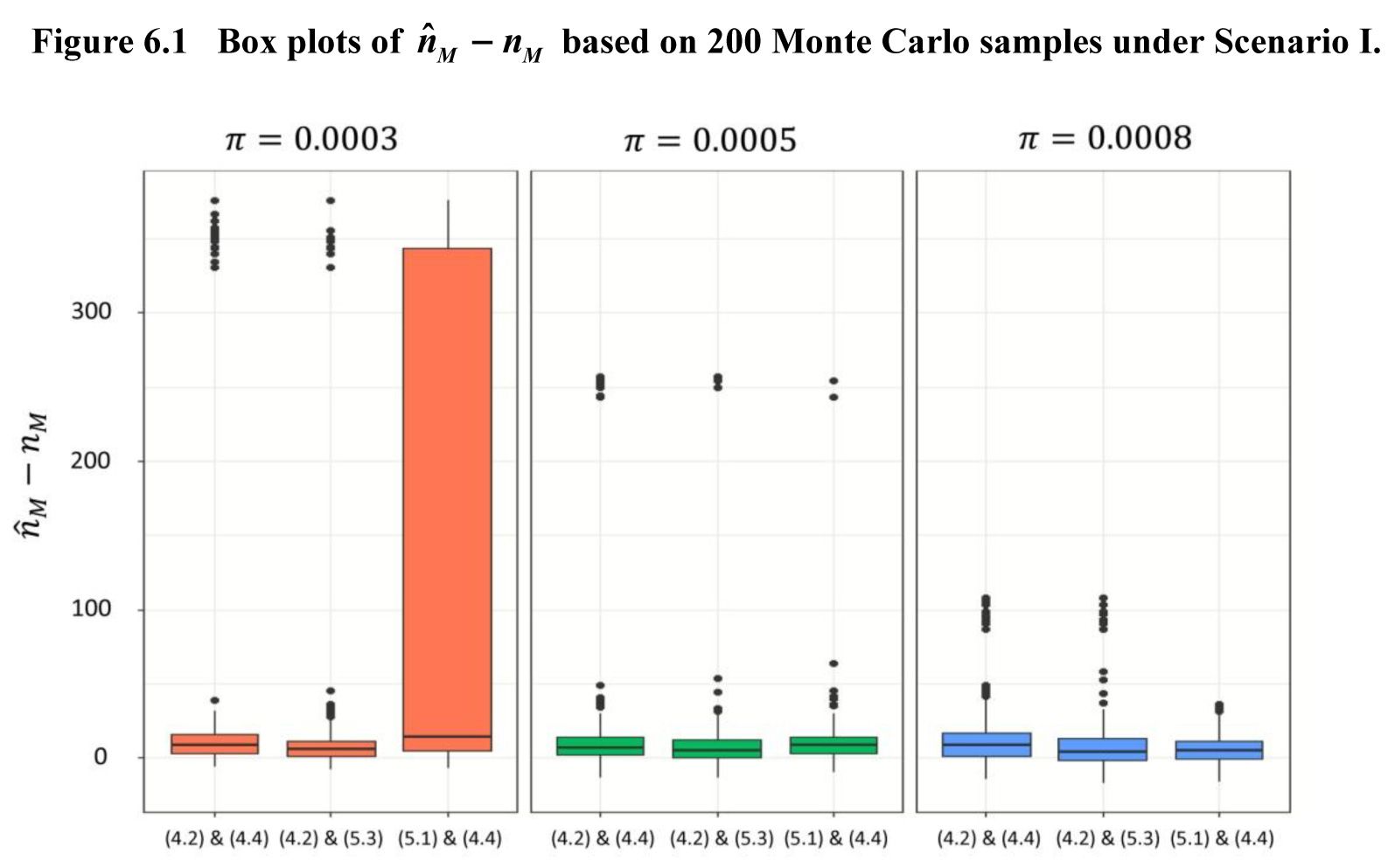
The results suggest that the unsupervised MEC algorithm tends to be more affected by the size of the matched set under Scenario-I than Scenario-II. Choosing (4.2) and (5.3), however, seems to yield the most robust estimation of n M MathType@MTEF@5@5@+= feaagKart1ev2aqatCvAUfeBSjuyZL2yd9gzLbvyNv2CaerbuLwBLn hiov2DGi1BTfMBaeXatLxBI9gBaerbd9wDYLwzYbItLDharqqtubsr 4rNCHbGeaGqiFu0Je9sqqrpepC0xbbf9F4rqqrFfpeea0xe9Lq=Jc9 vqaqpepm0xbba9pwe9Q8fs0=yqaqpepae9pg0FirpepeKkFr0xfr=x fr=xb9adbaqaaeGaciGaaiaabeqaamaabaabaaGcbaGaamOBamaaBa aaleaacaWGnbaabeaaaaa@37DA@  and error rates against the small size of the matched set M, MathType@MTEF@5@5@+= feaagKart1ev2aqatCvAUfeBSjuyZL2yd9gzLbvyNv2CaerbuLwBLn hiov2DGi1BTfMBaeXatLxBI9gBaerbd9wDYLwzYbItLDharqqtubsr 4rNCHbGeaGqiFu0Je9sqqrpepC0xbbf9F4rqqrFfpeea0xe9Lq=Jc9 vqaqpepm0xbba9pwe9Q8fs0=yqaqpepae9pg0FirpepeKkFr0xfr=x fr=xb9adbaqaaeGaciGaaiaabeqaamaabaabaaGcbaGaamytaiaacY caaaa@376B@  regardless the informativeness of key-variable errors. The reason must be the fact that the numerator of θ k ( t ) MathType@MTEF@5@5@+= feaagKart1ev2aqatCvAUfeBSjuyZL2yd9gzLbvyNv2CaerbuLwBLn hiov2DGi1BTfMBaeXatLxBI9gBaerbd9wDYLwzYbItLDharqqtubsr 4rNCHbGeaGqiFu0Je9sqqrpepC0xbbf9F4rqqrFfpeea0xe9Lq=Jc9 vqaqpepm0xbba9pwe9Q8fs0=yqaqpepae9pg0FirpepeKkFr0xfr=x fr=xb9adbaqaaeGaciGaaiaabeqaamaabaabaaGcbaGaeqiUde3aa0 baaSqaaiaadUgaaeaadaqadeqaaiaadshaaiaawIcacaGLPaaaaaaa aa@3B3F@  is calculated in (5.1) over all the pairs in Ω MathType@MTEF@5@5@+= feaagKart1ev2aqatCvAUfeBSjuyZL2yd9gzLbvyNv2CaerbuLwBLn hiov2DGi1BTfMBaeXatLxBI9gBaerbd9wDYLwzYbItLDharqqtubsr 4rNCHbGeaGqiFu0Je9sqqrpepC0xbbf9F4rqqrFfpeea0xe9Lq=Jc9 vqaqpepm0xbba9pwe9Q8fs0=yqaqpepae9pg0FirpepeKkFr0xfr=x fr=xb9adbaqaaeGaciGaaiaabeqaamaabaabaaGcbaGaeuyQdCfaaa@3777@  instead of the MEC set M ( t ) , MathType@MTEF@5@5@+= feaagKart1ev2aqatCvAUfeBSjuyZL2yd9gzLbvyNv2CaerbuLwBLn hiov2DGi1BTfMBaeXatLxBI9gBaerbd9wDYLwzYbItLDharqqtubsr 4rNCHbGeaGqiFu0Je9sqqrpepC0xbbf9F4rqqrFfpeea0xe9Lq=Jc9 vqaqpepm0xbba9pwe9Q8fs0=yqaqpepae9pg0FirpepeKkFr0xfr=x fr=xb9adbaqaaeGaciGaaiaabeqaamaabaabaaGcbaGaamytamaaCa aaleqabaWaaeWabeaacaWG0baacaGLOaGaayzkaaaaaOGaaiilaaaa @3A25@  which seems more sensitive when the imbalance between M MathType@MTEF@5@5@+= feaagKart1ev2aqatCvAUfeBSjuyZL2yd9gzLbvyNv2CaerbuLwBLn hiov2DGi1BTfMBaeXatLxBI9gBaerbd9wDYLwzYbItLDharqqtubsr 4rNCHbGeaGqiFu0Je9sqqrpepC0xbbf9F4rqqrFfpeea0xe9Lq=Jc9 vqaqpepm0xbba9pwe9Q8fs0=yqaqpepae9pg0FirpepeKkFr0xfr=x fr=xb9adbaqaaeGaciGaaiaabeqaamaabaabaaGcbaGaamytaaaa@36BB@  and U MathType@MTEF@5@5@+= feaagKart1ev2aqatCvAUfeBSjuyZL2yd9gzLbvyNv2CaerbuLwBLn hiov2DGi1BTfMBaeXatLxBI9gBaerbd9wDYLwzYbItLDharqqtubsr 4rNCHbGeaGqiFu0Je9sqqrpepC0xbbf9F4rqqrFfpeea0xe9Lq=Jc9 vqaqpepm0xbba9pwe9Q8fs0=yqaqpepae9pg0FirpepeKkFr0xfr=x fr=xb9adbaqaaeGaciGaaiaabeqaamaabaabaaGcbaGaamyvaaaa@36C3@  is aggravated, while the sizes of A MathType@MTEF@5@5@+= feaagKart1ev2aqatCvAUfeBSjuyZL2yd9gzLbvyNv2CaerbuLwBLn hiov2DGi1BTfMBaeXatLxBI9gBaerbd9wDYLwzYbItLDharqqtubsr 4rNCHbGeaGqiFu0Je9sqqrpepC0xbbf9F4rqqrFfpeea0xe9Lq=Jc9 vqaqpepm0xbba9pwe9Q8fs0=yqaqpepae9pg0FirpepeKkFr0xfr=x fr=xb9adbaqaaeGaciGaaiaabeqaamaabaabaaGcbaGaamyqaaaa@36AF@  and B MathType@MTEF@5@5@+= feaagKart1ev2aqatCvAUfeBSjuyZL2yd9gzLbvyNv2CaerbuLwBLn hiov2DGi1BTfMBaeXatLxBI9gBaerbd9wDYLwzYbItLDharqqtubsr 4rNCHbGeaGqiFu0Je9sqqrpepC0xbbf9F4rqqrFfpeea0xe9Lq=Jc9 vqaqpepm0xbba9pwe9Q8fs0=yqaqpepae9pg0FirpepeKkFr0xfr=x fr=xb9adbaqaaeGaciGaaiaabeqaamaabaabaaGcbaGaamOqaaaa@36B0@  remain fixed.
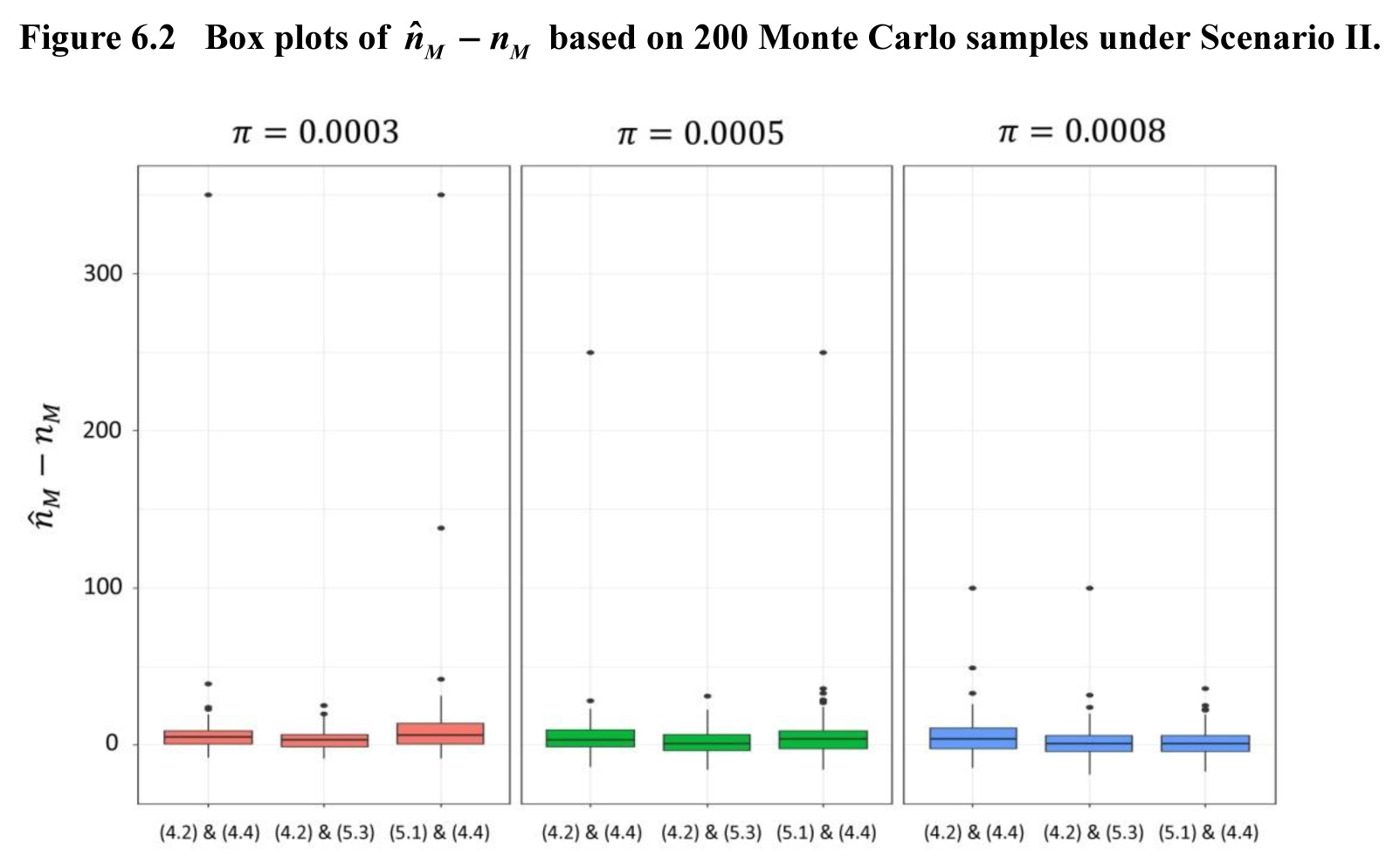
Figure 6.1

Description of Figure 6.1

Figure presenting box plots of n ^ M n M MathType@MTEF@5@5@+= feaagKart1ev2aqatCvAUfeBSjuyZL2yd9gzLbvyNv2CaerbuLwBLn hiov2DGi1BTfMBaeXatLxBI9gBaerbd9wDYLwzYbItLDharqqtubsr 4rNCHbGeaGqiFu0Je9sqqrpepC0xbbf9F4rqqrFfpC0xe9LqFHe9Lq pepeea0xd9q8as0=LqLs=Jirpepeea0=as0Fb9pgea0lrP0xe9Fve9 Fve9qapdbaqaaeGaciGaaiaabeqaamaabaabaaGcbaGabmOBayaaja WaaSbaaSqaaiaad2eaaeqaaOGaeyOeI0IaamOBamaaBaaaleaacaWG nbaabeaaaaa@3D53@  (the error of n ^ M ) MathType@MTEF@5@5@+= feaagKart1ev2aqatCvAUfeBSjuyZL2yd9gzLbvyNv2CaerbuLwBLn hiov2DGi1BTfMBaeXatLxBI9gBaerbd9wDYLwzYbItLDharqqtubsr 4rNCHbGeaGqiFu0Je9sqqrpepC0xbbf9F4rqqrFfpC0xe9LqFHe9Lq pepeea0xd9q8as0=LqLs=Jirpepeea0=as0Fb9pgea0lrP0xe9Fve9 Fve9qapdbaqaaeGaciGaaiaabeqaamaabaabaaGcbaGabmOBayaaja WaaSbaaSqaaiaad2eaaeqaaOGaaiykaaaa@3B22@  according to the use of different formulas ((4.2) and (4.4), (4.2) and (5.3), then (5.1) and (4.4)) for the prevalence of true matches π MathType@MTEF@5@5@+= feaagKart1ev2aqatCvAUfeBSjuyZL2yd9gzLbvyNv2CaerbuLwBLn hiov2DGi1BTfMBaeXatLxBI9gBaerbd9wDYLwzYbItLDharqqtubsr 4rNCHbGeaGqiFu0Je9sqqrpepC0xbbf9F4rqqrFfpC0xe9LqFHe9Lq pepeea0xd9q8as0=LqLs=Jirpepeea0=as0Fb9pgea0lrP0xe9Fve9 Fve9qapdbaqaaeGaciGaaiaabeqaamaabaabaaGcbaGaeqiWdahaaa@3A27@  equal to 0.0003 (orange), 0.0005 (green) and 0.0008 (blue) based on 200 Monte Carlo samples under Scenario I. In general, the estimate n ^ M MathType@MTEF@5@5@+= feaagKart1ev2aqatCvAUfeBSjuyZL2yd9gzLbvyNv2CaerbuLwBLn hiov2DGi1BTfMBaeXatLxBI9gBaerbd9wDYLwzYbItLDharqqtubsr 4rNCHbGeaGqiFu0Je9sqqrpepC0xbbf9F4rqqrFfpC0xe9LqFHe9Lq pepeea0xd9q8as0=LqLs=Jirpepeea0=as0Fb9pgea0lrP0xe9Fve9 Fve9qapdbaqaaeGaciGaaiaabeqaamaabaabaaGcbaGabmOBayaaja WaaSbaaSqaaiaad2eaaeqaaaaa@3A6B@  gets worse as π MathType@MTEF@5@5@+= feaagKart1ev2aqatCvAUfeBSjuyZL2yd9gzLbvyNv2CaerbuLwBLn hiov2DGi1BTfMBaeXatLxBI9gBaerbd9wDYLwzYbItLDharqqtubsr 4rNCHbGeaGqiFu0Je9sqqrpepC0xbbf9F4rqqrFfpC0xe9LqFHe9Lq pepeea0xd9q8as0=LqLs=Jirpepeea0=as0Fb9pgea0lrP0xe9Fve9 Fve9qapdbaqaaeGaciGaaiaabeqaamaabaabaaGcbaGaeqiWdahaaa@3A27@  reduces. Choosing (4.2) and (5.3) seems to yield the most robust estimation of n M . MathType@MTEF@5@5@+= feaagKart1ev2aqatCvAUfeBSjuyZL2yd9gzLbvyNv2CaerbuLwBLn hiov2DGi1BTfMBaeXatLxBI9gBaerbd9wDYLwzYbItLDharqqtubsr 4rNCHbGeaGqiFu0Je9sqqrpepC0xbbf9F4rqqrFfpC0xe9LqFHe9Lq pepeea0xd9q8as0=LqLs=Jirpepeea0=as0Fb9pgea0lrP0xe9Fve9 Fve9qapdbaqaaeGaciGaaiaabeqaamaabaabaaGcbaGaamOBamaaBa aaleaacaWGnbaabeaakiaac6caaaa@3B17@

Figure 6.2

Description of Figure 6.2

Figure presenting box plots of n ^ M n M MathType@MTEF@5@5@+= feaagKart1ev2aqatCvAUfeBSjuyZL2yd9gzLbvyNv2CaerbuLwBLn hiov2DGi1BTfMBaeXatLxBI9gBaerbd9wDYLwzYbItLDharqqtubsr 4rNCHbGeaGqiFu0Je9sqqrpepC0xbbf9F4rqqrFfpC0xe9LqFHe9Lq pepeea0xd9q8as0=LqLs=Jirpepeea0=as0Fb9pgea0lrP0xe9Fve9 Fve9qapdbaqaaeGaciGaaiaabeqaamaabaabaaGcbaGabmOBayaaja WaaSbaaSqaaiaad2eaaeqaaOGaeyOeI0IaamOBamaaBaaaleaacaWG nbaabeaaaaa@3D53@  (the error of n ^ M ) MathType@MTEF@5@5@+= feaagKart1ev2aqatCvAUfeBSjuyZL2yd9gzLbvyNv2CaerbuLwBLn hiov2DGi1BTfMBaeXatLxBI9gBaerbd9wDYLwzYbItLDharqqtubsr 4rNCHbGeaGqiFu0Je9sqqrpepC0xbbf9F4rqqrFfpC0xe9LqFHe9Lq pepeea0xd9q8as0=LqLs=Jirpepeea0=as0Fb9pgea0lrP0xe9Fve9 Fve9qapdbaqaaeGaciGaaiaabeqaamaabaabaaGcbaGabmOBayaaja WaaSbaaSqaaiaad2eaaeqaaOGaaiykaaaa@3B22@  according to the use of different formulas ((4.2) and (4.4), (4.2) and (5.3), then (5.1) and (4.4)) for the prevalence of true matches π MathType@MTEF@5@5@+= feaagKart1ev2aqatCvAUfeBSjuyZL2yd9gzLbvyNv2CaerbuLwBLn hiov2DGi1BTfMBaeXatLxBI9gBaerbd9wDYLwzYbItLDharqqtubsr 4rNCHbGeaGqiFu0Je9sqqrpepC0xbbf9F4rqqrFfpC0xe9LqFHe9Lq pepeea0xd9q8as0=LqLs=Jirpepeea0=as0Fb9pgea0lrP0xe9Fve9 Fve9qapdbaqaaeGaciGaaiaabeqaamaabaabaaGcbaGaeqiWdahaaa@3A27@  equal to 0.0003 (orange), 0.0005 (green) and 0.0008 (blue) based on 200 Monte Carlo samples under Scenario II. In general, the estimate n ^ M MathType@MTEF@5@5@+= feaagKart1ev2aqatCvAUfeBSjuyZL2yd9gzLbvyNv2CaerbuLwBLn hiov2DGi1BTfMBaeXatLxBI9gBaerbd9wDYLwzYbItLDharqqtubsr 4rNCHbGeaGqiFu0Je9sqqrpepC0xbbf9F4rqqrFfpC0xe9LqFHe9Lq pepeea0xd9q8as0=LqLs=Jirpepeea0=as0Fb9pgea0lrP0xe9Fve9 Fve9qapdbaqaaeGaciGaaiaabeqaamaabaabaaGcbaGabmOBayaaja WaaSbaaSqaaiaad2eaaeqaaaaa@3A6B@  gets worse as π MathType@MTEF@5@5@+= feaagKart1ev2aqatCvAUfeBSjuyZL2yd9gzLbvyNv2CaerbuLwBLn hiov2DGi1BTfMBaeXatLxBI9gBaerbd9wDYLwzYbItLDharqqtubsr 4rNCHbGeaGqiFu0Je9sqqrpepC0xbbf9F4rqqrFfpC0xe9LqFHe9Lq pepeea0xd9q8as0=LqLs=Jirpepeea0=as0Fb9pgea0lrP0xe9Fve9 Fve9qapdbaqaaeGaciGaaiaabeqaamaabaabaaGcbaGaeqiWdahaaa@3A27@  reduces. Choosing (4.2) and (5.3) seems to yield the most robust estimation of n M . MathType@MTEF@5@5@+= feaagKart1ev2aqatCvAUfeBSjuyZL2yd9gzLbvyNv2CaerbuLwBLn hiov2DGi1BTfMBaeXatLxBI9gBaerbd9wDYLwzYbItLDharqqtubsr 4rNCHbGeaGqiFu0Je9sqqrpepC0xbbf9F4rqqrFfpC0xe9LqFHe9Lq pepeea0xd9q8as0=LqLs=Jirpepeea0=as0Fb9pgea0lrP0xe9Fve9 Fve9qapdbaqaaeGaciGaaiaabeqaamaabaabaaGcbaGaamOBamaaBa aaleaacaWGnbaabeaakiaac6caaaa@3B17@  The results suggest that the unsupervised Maximum Entropy Classification algorithm tends to be more affected by the size of the matched set under Scenario I than Scenario II.

We also include the additional results obtained for p A =0.2,0.15, MathType@MTEF@5@5@+= feaagKart1ev2aqatCvAUfeBSjuyZL2yd9gzLbvyNv2CaerbuLwBLn hiov2DGi1BTfMBaeXatLxBI9gBaerbd9wDYLwzYbItLDharqqtubsr 4rNCHbGeaGqiFu0Je9sqqrpepC0xbbf9F4rqqrFfpeea0xe9Lq=Jc9 vqaqpepm0xbba9pwe9Q8fs0=yqaqpepae9pg0FirpepeKkFr0xfr=x fr=xb9adbaqaaeGaciGaaiaabeqaamaabaabaaGcbaGaamiCamaaBa aaleaacaWGbbaabeaakiaaysW7cqGH9aqpcaaMc8UaaGPaVlaaicda caGGUaGaaGOmaiaacYcacaaMc8UaaGPaVlaaicdacaGGUaGaaGymai aaiwdacaGGSaaaaa@4707@  and 0.1 in the supplementary material. The estimate n ^ M MathType@MTEF@5@5@+= feaagKart1ev2aqatCvAUfeBSjuyZL2yd9gzLbvyNv2CaerbuLwBLn hiov2DGi1BTfMBaeXatLxBI9gBaerbd9wDYLwzYbItLDharqqtubsr 4rNCHbGeaGqiFu0Je9sqqrpepC0xbbf9F4rqqrFfpeea0xe9Lq=Jc9 vqaqpepm0xbba9pwe9Q8fs0=yqaqpepae9pg0FirpepeKkFr0xfr=x fr=xb9adbaqaaeGaciGaaiaabeqaamaabaabaaGcbaGabmOBayaaja WaaSbaaSqaaiaad2eaaeqaaaaa@37EA@  (or π ^ ) MathType@MTEF@5@5@+= feaagKart1ev2aqatCvAUfeBSjuyZL2yd9gzLbvyNv2CaerbuLwBLn hiov2DGi1BTfMBaeXatLxBI9gBaerbd9wDYLwzYbItLDharqqtubsr 4rNCHbGeaGqiFu0Je9sqqrpepC0xbbf9F4rqqrFfpeea0xe9Lq=Jc9 vqaqpepm0xbba9pwe9Q8fs0=yqaqpepae9pg0FirpepeKkFr0xfr=x fr=xb9adbaqaaeGaciGaaiaabeqaamaabaabaaGcbaGafqiWdaNbaK aacaGGPaaaaa@3863@  gets worse as p A MathType@MTEF@5@5@+= feaagKart1ev2aqatCvAUfeBSjuyZL2yd9gzLbvyNv2CaerbuLwBLn hiov2DGi1BTfMBaeXatLxBI9gBaerbd9wDYLwzYbItLDharqqtubsr 4rNCHbGeaGqiFu0Je9sqqrpepC0xbbf9F4rqqrFfpeea0xe9Lq=Jc9 vqaqpepm0xbba9pwe9Q8fs0=yqaqpepae9pg0FirpepeKkFr0xfr=x fr=xb9adbaqaaeGaciGaaiaabeqaamaabaabaaGcbaGaamiCamaaBa aaleaacaWGbbaabeaaaaa@37D0@  (or π) MathType@MTEF@5@5@+= feaagKart1ev2aqatCvAUfeBSjuyZL2yd9gzLbvyNv2CaerbuLwBLn hiov2DGi1BTfMBaeXatLxBI9gBaerbd9wDYLwzYbItLDharqqtubsr 4rNCHbGeaGqiFu0Je9sqqrpepC0xbbf9F4rqqrFfpeea0xe9Lq=Jc9 vqaqpepm0xbba9pwe9Q8fs0=yqaqpepae9pg0FirpepeKkFr0xfr=x fr=xb9adbaqaaeGaciGaaiaabeqaamaabaabaaGcbaGaeqiWdaNaai ykaaaa@3853@  reduces, which is consistent with the previous findings of others, for example, Enamorado, Fifield and Imai (2019) showed that a greater degree of overlap between data sets leads to better merging results in terms of the error rates as well as the accuracy of their estimates. The problem is also highlighted by Sadinle (2017). Record linkage in cases of extremely low prevalence of true matches is a problem that needs to be studied more carefully on its own.

6.3   Results: MEC set

Aiming the MEC set M ^ MathType@MTEF@5@5@+= feaagKart1ev2aqatCvAUfeBSjuyZL2yd9gzLbvyNv2CaerbuLwBLn hiov2DGi1BTfMBaeXatLxBI9gBaerbd9wDYLwzYbItLDharqqtubsr 4rNCHbGeaGqiFu0Je9sqqrpepC0xbbf9F4rqqrFfpeea0xe9Lq=Jc9 vqaqpepm0xbba9pwe9Q8fs0=yqaqpepae9pg0FirpepeKkFr0xfr=x fr=xb9adbaqaaeGaciGaaiaabeqaamaabaabaaGcbaGabmytayaaja aaaa@36CB@  at the estimated size n ^ M MathType@MTEF@5@5@+= feaagKart1ev2aqatCvAUfeBSjuyZL2yd9gzLbvyNv2CaerbuLwBLn hiov2DGi1BTfMBaeXatLxBI9gBaerbd9wDYLwzYbItLDharqqtubsr 4rNCHbGeaGqiFu0Je9sqqrpepC0xbbf9F4rqqrFfpeea0xe9Lq=Jc9 vqaqpepm0xbba9pwe9Q8fs0=yqaqpepae9pg0FirpepeKkFr0xfr=x fr=xb9adbaqaaeGaciGaaiaabeqaamaabaabaaGcbaGabmOBayaaja WaaSbaaSqaaiaad2eaaeqaaaaa@37EA@  is generally not a reasonable approach to record linkage. Record linkage should be guided directly by the associated uncertainty, i.e. the error rates FLR and MMR, based on their estimates (4.5) and (4.6), as described in Section 4.2. Note that this does require the estimation of n M MathType@MTEF@5@5@+= feaagKart1ev2aqatCvAUfeBSjuyZL2yd9gzLbvyNv2CaerbuLwBLn hiov2DGi1BTfMBaeXatLxBI9gBaerbd9wDYLwzYbItLDharqqtubsr 4rNCHbGeaGqiFu0Je9sqqrpepC0xbbf9F4rqqrFfpeea0xe9Lq=Jc9 vqaqpepm0xbba9pwe9Q8fs0=yqaqpepae9pg0FirpepeKkFr0xfr=x fr=xb9adbaqaaeGaciGaaiaabeqaamaabaabaaGcbaGaamOBamaaBa aaleaacaWGnbaabeaaaaa@37DA@  in addition to r( γ ). MathType@MTEF@5@5@+= feaagKart1ev2aqatCvAUfeBSjuyZL2yd9gzLbvyNv2CaerbuLwBLn hiov2DGi1BTfMBaeXatLxBI9gBaerbd9wDYLwzYbItLDharqqtubsr 4rNCHbGeaGqiFu0Je9sqqrpepC0xbbf9F4rqqrFfpeea0xe9Lq=Jc9 vqaqpepm0xbba9pwe9Q8fs0=yqaqpepae9pg0FirpepeKkFr0xfr=x fr=xb9adbaqaaeGaciGaaiaabeqaamaabaabaaGcbaGaamOCaiaayk W7daqadeqaaiaaho7aaiaawIcacaGLPaaacaGGUaaaaa@3BE6@

We have FLR ^ MathType@MTEF@5@5@+= feaagKart1ev2aqatCvAUfeBSjuyZL2yd9gzLbvyNv2CaerbuLwBLn hiov2DGi1BTfMBaeXatLxBI9gBaerbd9wDYLwzYbItLDharqqtubsr 4rNCHbGeaGqiVu0Je9sqqrpepC0xbbL8F4rqqrFfpeea0xe9Lq=Jc9 vqaqpepm0xbba9pwe9Q8fs0=yqaqpepae9pg0FirpepeKkFr0xfr=x fr=xb9adbaqaaeGaciGaaiaabeqaamaabaabaaGcbaWaaecaaeaaqa aaaaaaaaWdbiaaboeacaqGqbGaae4taaWdaiaawkWaamaaBaaaleaa peGaamyAaaWdaeqaaaaa@3A8C@ = MathType@MTEF@5@5@+= feaagKart1ev2aqatCvAUfeBSjuyZL2yd9gzLbvyNv2CaerbuLwBLn hiov2DGi1BTfMBaeXatLxBI9gBaerbd9wDYLwzYbItLDharqqtubsr 4rNCHbGeaGqiVu0Je9sqqrpepC0xbbL8F4rqqrFfpeea0xe9Lq=Jc9 vqaqpepm0xbba9pwe9Q8fs0=yqaqpepae9pg0FirpepeKkFr0xfr=x fr=xb9adbaqaaeGaciGaaiaabeqaamaabaabaaGcbaaeaaaaaaaaa8 qacqGH9aqpaaa@371D@ MMR ^ MathType@MTEF@5@5@+= feaagKart1ev2aqatCvAUfeBSjuyZL2yd9gzLbvyNv2CaerbuLwBLn hiov2DGi1BTfMBaeXatLxBI9gBaerbd9wDYLwzYbItLDharqqtubsr 4rNCHbGeaGqiVu0Je9sqqrpepC0xbbL8F4rqqrFfpeea0xe9Lq=Jc9 vqaqpepm0xbba9pwe9Q8fs0=yqaqpepae9pg0FirpepeKkFr0xfr=x fr=xb9adbaqaaeGaciGaaiaabeqaamaabaabaaGcbaWaaecaaeaaqa aaaaaaaaWdbiaaboeacaqGqbGaae4taaWdaiaawkWaamaaBaaaleaa peGaamyAaaWdaeqaaaaa@3A8C@  in Table 6.3, because | M ^ |= n ^ M MathType@MTEF@5@5@+= feaagKart1ev2aqatCvAUfeBSjuyZL2yd9gzLbvyNv2CaerbuLwBLn hiov2DGi1BTfMBaeXatLxBI9gBaerbd9wDYLwzYbItLDharqqtubsr 4rNCHbGeaGqiFu0Je9sqqrpepC0xbbf9F4rqqrFfpeea0xe9Lq=Jc9 vqaqpepm0xbba9pwe9Q8fs0=yqaqpepae9pg0FirpepeKkFr0xfr=x fr=xb9adbaqaaeGaciGaaiaabeqaamaabaabaaGcbaWaaqWabeaaca aMc8UabmytayaajaGaaGPaVdGaay5bSlaawIa7aiaaysW7cqGH9aqp caaMe8UabmOBayaajaWaaSbaaSqaaiaad2eaaeqaaaaa@4325@  here. It can be seen that these follow the true FLR more closely than the MMR, especially when n ^ M MathType@MTEF@5@5@+= feaagKart1ev2aqatCvAUfeBSjuyZL2yd9gzLbvyNv2CaerbuLwBLn hiov2DGi1BTfMBaeXatLxBI9gBaerbd9wDYLwzYbItLDharqqtubsr 4rNCHbGeaGqiFu0Je9sqqrpepC0xbbf9F4rqqrFfpeea0xe9Lq=Jc9 vqaqpepm0xbba9pwe9Q8fs0=yqaqpepae9pg0FirpepeKkFr0xfr=x fr=xb9adbaqaaeGaciGaaiaabeqaamaabaabaaGcbaGabmOBayaaja WaaSbaaSqaaiaad2eaaeqaaaaa@37EA@  is estimated using the formulae (4.2) and (5.3). This is hardly surprising. Take e.g. the maximal MEC set M 1 MathType@MTEF@5@5@+= feaagKart1ev2aqatCvAUfeBSjuyZL2yd9gzLbvyNv2CaerbuLwBLn hiov2DGi1BTfMBaeXatLxBI9gBaerbd9wDYLwzYbItLDharqqtubsr 4rNCHbGeaGqiFu0Je9sqqrpepC0xbbf9F4rqqrFfpeea0xe9Lq=Jc9 vqaqpepm0xbba9pwe9Q8fs0=yqaqpepae9pg0FirpepeKkFr0xfr=x fr=xb9adbaqaaeGaciGaaiaabeqaamaabaabaaGcbaGaamytamaaBa aaleaacaaIXaaabeaaaaa@37A2@  that consists of the pairs whose key variables agree completely and uniquely. Provided reasonably rich key variables, as the setting here, one can expect the FLR of M 1 MathType@MTEF@5@5@+= feaagKart1ev2aqatCvAUfeBSjuyZL2yd9gzLbvyNv2CaerbuLwBLn hiov2DGi1BTfMBaeXatLxBI9gBaerbd9wDYLwzYbItLDharqqtubsr 4rNCHbGeaGqiFu0Je9sqqrpepC0xbbf9F4rqqrFfpeea0xe9Lq=Jc9 vqaqpepm0xbba9pwe9Q8fs0=yqaqpepae9pg0FirpepeKkFr0xfr=x fr=xb9adbaqaaeGaciGaaiaabeqaamaabaabaaGcbaGaamytamaaBa aaleaacaaIXaaabeaaaaa@37A2@  to be low, such that even a naïve estimate FLR ^ MathType@MTEF@5@5@+= feaagKart1ev2aqatCvAUfeBSjuyZL2yd9gzLbvyNv2CaerbuLwBLn hiov2DGi1BTfMBaeXatLxBI9gBaerbd9wDYLwzYbItLDharqqtubsr 4rNCHbGeaGqiVu0Je9sqqrpepC0xbbL8F4rqqrFfpeea0xe9Lq=Jc9 vqaqpepm0xbba9pwe9Q8fs0=yqaqpepae9pg0FirpepeKkFr0xfr=x fr=xb9adbaqaaeGaciGaaiaabeqaamaabaabaaGcbaWaaecaaeaaqa aaaaaaaaWdbiaaboeacaqGqbGaae4taaWdaiaawkWaamaaBaaaleaa peGaamyAaaWdaeqaaaaa@3A8C@ =0 MathType@MTEF@5@5@+= feaagKart1ev2aqatCvAUfeBSjuyZL2yd9gzLbvyNv2CaerbuLwBLn hiov2DGi1BTfMBaeXatLxBI9gBaerbd9wDYLwzYbItLDharqqtubsr 4rNCHbGeaGqiVu0Je9sqqrpepC0xbbL8F4rqqrFfpeea0xe9Lq=Jc9 vqaqpepm0xbba9pwe9Q8fs0=yqaqpepae9pg0FirpepeKkFr0xfr=x fr=xb9adbaqaaeGaciGaaiaabeqaamaabaabaaGcbaaeaaaaaaaaa8 qacqGH9aqpcaaIWaaaaa@37D7@  probably does not err much. Meanwhile, the true MMR has a much wider range from one application to another, because the difference between n M MathType@MTEF@5@5@+= feaagKart1ev2aqatCvAUfeBSjuyZL2yd9gzLbvyNv2CaerbuLwBLn hiov2DGi1BTfMBaeXatLxBI9gBaerbd9wDYLwzYbItLDharqqtubsr 4rNCHbGeaGqiFu0Je9sqqrpepC0xbbf9F4rqqrFfpeea0xe9Lq=Jc9 vqaqpepm0xbba9pwe9Q8fs0=yqaqpepae9pg0FirpepeKkFr0xfr=x fr=xb9adbaqaaeGaciGaaiaabeqaamaabaabaaGcbaGaamOBamaaBa aaleaacaWGnbaabeaaaaa@37DA@  and | M 1 | MathType@MTEF@5@5@+= feaagKart1ev2aqatCvAUfeBSjuyZL2yd9gzLbvyNv2CaerbuLwBLn hiov2DGi1BTfMBaeXatLxBI9gBaerbd9wDYLwzYbItLDharqqtubsr 4rNCHbGeaGqiFu0Je9sqqrpepC0xbbf9F4rqqrFfpeea0xe9Lq=Jc9 vqaqpepm0xbba9pwe9Q8fs0=yqaqpepae9pg0FirpepeKkFr0xfr=x fr=xb9adbaqaaeGaciGaaiaabeqaamaabaabaaGcbaWaaqWabeaaca aMc8UaamytamaaBaaaleaacaaIXaaabeaakiaaykW7aiaawEa7caGL iWoaaaa@3DE5@  is determined by the extent of key-variable errors, such that the estimate of MMR depends more critically on that of n M . MathType@MTEF@5@5@+= feaagKart1ev2aqatCvAUfeBSjuyZL2yd9gzLbvyNv2CaerbuLwBLn hiov2DGi1BTfMBaeXatLxBI9gBaerbd9wDYLwzYbItLDharqqtubsr 4rNCHbGeaGqiFu0Je9sqqrpepC0xbbf9F4rqqrFfpeea0xe9Lq=Jc9 vqaqpepm0xbba9pwe9Q8fs0=yqaqpepae9pg0FirpepeKkFr0xfr=x fr=xb9adbaqaaeGaciGaaiaabeqaamaabaabaaGcbaGaamOBamaaBa aaleaacaWGnbaabeaakiaac6caaaa@3896@  The situation is similar for any MEC set beyond M 1 , MathType@MTEF@5@5@+= feaagKart1ev2aqatCvAUfeBSjuyZL2yd9gzLbvyNv2CaerbuLwBLn hiov2DGi1BTfMBaeXatLxBI9gBaerbd9wDYLwzYbItLDharqqtubsr 4rNCHbGeaGqiFu0Je9sqqrpepC0xbbf9F4rqqrFfpeea0xe9Lq=Jc9 vqaqpepm0xbba9pwe9Q8fs0=yqaqpepae9pg0FirpepeKkFr0xfr=x fr=xb9adbaqaaeGaciGaaiaabeqaamaabaabaaGcbaGaamytamaaBa aaleaacaaIXaaabeaakiaacYcaaaa@385C@  as long as g ^ ab MathType@MTEF@5@5@+= feaagKart1ev2aqatCvAUfeBSjuyZL2yd9gzLbvyNv2CaerbuLwBLn hiov2DGi1BTfMBaeXatLxBI9gBaerbd9wDYLwzYbItLDharqqtubsr 4rNCHbGeaGqiFu0Je9sqqrpepC0xbbf9F4rqqrFfpeea0xe9Lq=Jc9 vqaqpepm0xbba9pwe9Q8fs0=yqaqpepae9pg0FirpepeKkFr0xfr=x fr=xb9adbaqaaeGaciGaaiaabeqaamaabaabaaGcbaGabm4zayaaja WaaSbaaSqaaiaadggacaWGIbaabeaaaaa@38DE@  remains very high for any ( a,b ) M ^ . MathType@MTEF@5@5@+= feaagKart1ev2aqatCvAUfeBSjuyZL2yd9gzLbvyNv2CaerbuLwBLn hiov2DGi1BTfMBaeXatLxBI9gBaerbd9wDYLwzYbItLDharqqtubsr 4rNCHbGeaGqiFu0Je9sqqrpepC0xbbf9F4rqqrFfpeea0xe9Lq=Jc9 vqaqpepm0xbba9pwe9Q8fs0=yqaqpepae9pg0FirpepeKkFr0xfr=x fr=xb9adbaqaaeGaciGaaiaabeqaamaabaabaaGcbaWaaeWabeaaca WGHbGaaGilaiaaysW7caWGIbaacaGLOaGaayzkaaGaaGjbVlabgIGi olaaysW7ceWGnbGbaKaacaGGUaaaaa@41B5@

Table 6.4 shows the performance of the MEC set using the bisection procedure described in Section 4.2, across the same set-ups as in Table 6.3. We use only (4.2) for θ k ( t ) MathType@MTEF@5@5@+= feaagKart1ev2aqatCvAUfeBSjuyZL2yd9gzLbvyNv2CaerbuLwBLn hiov2DGi1BTfMBaeXatLxBI9gBaerbd9wDYLwzYbItLDharqqtubsr 4rNCHbGeaGqiFu0Je9sqqrpepC0xbbf9F4rqqrFfpeea0xe9Lq=Jc9 vqaqpepm0xbba9pwe9Q8fs0=yqaqpepae9pg0FirpepeKkFr0xfr=x fr=xb9adbaqaaeGaciGaaiaabeqaamaabaabaaGcbaGaeqiUde3aa0 baaSqaaiaadUgaaeaadaqadeqaaiaadshaaiaawIcacaGLPaaaaaaa aa@3B3F@  and (5.3) for ξ k ( t ) MathType@MTEF@5@5@+= feaagKart1ev2aqatCvAUfeBSjuyZL2yd9gzLbvyNv2CaerbuLwBLn hiov2DGi1BTfMBaeXatLxBI9gBaerbd9wDYLwzYbItLDharqqtubsr 4rNCHbGeaGqiFu0Je9sqqrpepC0xbbf9F4rqqrFfpeea0xe9Lq=Jc9 vqaqpepm0xbba9pwe9Q8fs0=yqaqpepae9pg0FirpepeKkFr0xfr=x fr=xb9adbaqaaeGaciGaaiaabeqaamaabaabaaGcbaGaeqOVdG3aa0 baaSqaaiaadUgaaeaadaqadeqaaiaadshaaiaawIcacaGLPaaaaaaa aa@3B4C@  to obtain the corresponding n ^ M . MathType@MTEF@5@5@+= feaagKart1ev2aqatCvAUfeBSjuyZL2yd9gzLbvyNv2CaerbuLwBLn hiov2DGi1BTfMBaeXatLxBI9gBaerbd9wDYLwzYbItLDharqqtubsr 4rNCHbGeaGqiFu0Je9sqqrpepC0xbbf9F4rqqrFfpeea0xe9Lq=Jc9 vqaqpepm0xbba9pwe9Q8fs0=yqaqpepae9pg0FirpepeKkFr0xfr=x fr=xb9adbaqaaeGaciGaaiaabeqaamaabaabaaGcbaGabmOBayaaja WaaSbaaSqaaiaad2eaaeqaaOGaaiOlaaaa@38A6@  We let the target FLR be ψ=0.05 MathType@MTEF@5@5@+= feaagKart1ev2aqatCvAUfeBSjuyZL2yd9gzLbvyNv2CaerbuLwBLn hiov2DGi1BTfMBaeXatLxBI9gBaerbd9wDYLwzYbItLDharqqtubsr 4rNCHbGeaGqiFu0Je9sqqrpepC0xbbf9F4rqqrFfpeea0xe9Lq=Jc9 vqaqpepm0xbba9pwe9Q8fs0=yqaqpepae9pg0FirpepeKkFr0xfr=x fr=xb9adbaqaaeGaciGaaiaabeqaamaabaabaaGcbaGaeqiYdKNaaG jbVlabg2da9iaaykW7caaMc8UaaGimaiaac6cacaaIWaGaaGynaaaa @4045@  or 0.03, where the latter is clearly lower than the true FLR of M ^ MathType@MTEF@5@5@+= feaagKart1ev2aqatCvAUfeBSjuyZL2yd9gzLbvyNv2CaerbuLwBLn hiov2DGi1BTfMBaeXatLxBI9gBaerbd9wDYLwzYbItLDharqqtubsr 4rNCHbGeaGqiFu0Je9sqqrpepC0xbbf9F4rqqrFfpeea0xe9Lq=Jc9 vqaqpepm0xbba9pwe9Q8fs0=yqaqpepae9pg0FirpepeKkFr0xfr=x fr=xb9adbaqaaeGaciGaaiaabeqaamaabaabaaGcbaGabmytayaaja aaaa@36CB@  that is of the size n ^ M MathType@MTEF@5@5@+= feaagKart1ev2aqatCvAUfeBSjuyZL2yd9gzLbvyNv2CaerbuLwBLn hiov2DGi1BTfMBaeXatLxBI9gBaerbd9wDYLwzYbItLDharqqtubsr 4rNCHbGeaGqiFu0Je9sqqrpepC0xbbf9F4rqqrFfpeea0xe9Lq=Jc9 vqaqpepm0xbba9pwe9Q8fs0=yqaqpepae9pg0FirpepeKkFr0xfr=x fr=xb9adbaqaaeGaciGaaiaabeqaamaabaabaaGcbaGabmOBayaaja WaaSbaaSqaaiaad2eaaeqaaaaa@37EA@  (Table 6.3), especially when the prevalence is relatively low (at π=0.0003) MathType@MTEF@5@5@+= feaagKart1ev2aqatCvAUfeBSjuyZL2yd9gzLbvyNv2CaerbuLwBLn hiov2DGi1BTfMBaeXatLxBI9gBaerbd9wDYLwzYbItLDharqqtubsr 4rNCHbGeaGqiFu0Je9sqqrpepC0xbbf9F4rqqrFfpeea0xe9Lq=Jc9 vqaqpepm0xbba9pwe9Q8fs0=yqaqpepae9pg0FirpepeKkFr0xfr=x fr=xb9adbaqaaeGaciGaaiaabeqaamaabaabaaGcbaGaeqiWdaNaaG jbVlabg2da9iaaykW7caaMc8UaaGimaiaac6cacaaIWaGaaGimaiaa icdacaaIZaGaaiykaaaa@4253@  under either scenario. The resulting true (FLR, MMR) and their estimates are given in Table 6.4.


Table 6.4
Parameters and averages of their estimates, averages of error rates and their estimates, over 200 simulations, n=| Ω |= n A n B MathType@MTEF@5@5@+= feaagKart1ev2aqatCvAUfeBSjuyZL2yd9gzLbvyNv2CaerbuLwBLn hiov2DGi1BTfMBaeXatLxBI9gBaerbd9wDYLwzYbItLDharqqtubsr 4rNCHbGeaGqipu0Je9sqqrpepC0xbbf9F4rqqrFfpeea0xe9Lq=Jc9 vqaqpepm0xbba9pwe9Q8fs0=yqaqpepae9pg0FirpepeKkFr0xfr=x fr=xb9adbeqabeWacmGabiqabeqabmqabeabbaGcbaGaamOBaiaays W7cqGH9aqpcaaMe8+aaqWabeaacaaMc8UaeuyQdCLaaGPaVdGaay5b SlaawIa7aiaaysW7cqGH9aqpcaaMe8UaamOBamaaBaaaleaacaWGbb aabeaakiaad6gadaWgaaWcbaGaamOqaaqabaaaaa@4AB2@
Table summary
This table displays the results of Parameters and averages of their estimates Scenario I and Scenario II (appearing as column headers).
Scenario I Scenario II
Parameter Target
FLR
Estimation Parameter Target
FLR
Estimation
π MathType@MTEF@5@5@+= feaagKart1ev2aqatCvAUfeBSjuyZL2yd9gzLbvyNv2CaerbuLwBLn hiov2DGi1BTfMBaeXatLxBI9gBaerbd9wDYLwzYbItLDharqqtubsr 4rNCHbGeaGWj0Jf9crFfpeea0xh9v8qqW7rqqrFfpeea0xe9Lq=Jc9 vqaqpepm0xbba9pwe9Q8fs0=yqaqpepae9pg0FirpepeKkFr0xfr=x fr=xb9adbeqabeWacmGabiqabeqabmqabeabbaGcbaGaeqiWdahaaa@39EF@ E( n M ) MathType@MTEF@5@5@+= feaagKart1ev2aqatCvAUfeBSjuyZL2yd9gzLbvyNv2CaerbuLwBLn hiov2DGi1BTfMBaeXatLxBI9gBaerbd9wDYLwzYbItLDharqqtubsr 4rNCHbGeaGWj0Jf9crFfpeea0xh9v8qqW7rqqrFfpeea0xe9Lq=Jc9 vqaqpepm0xbba9pwe9Q8fs0=yqaqpepae9pg0FirpepeKkFr0xfr=x fr=xb9adbeqabeWacmGabiqabeqabmqabeabbaGcbaGaamyraiaayk W7daqadeqaaiaad6gadaWgaaWcbaGaamytaaqabaaakiaawIcacaGL Paaaaaa@3E0C@ n ^ M MathType@MTEF@5@5@+= feaagKart1ev2aqatCvAUfeBSjuyZL2yd9gzLbvyNv2CaerbuLwBLn hiov2DGi1BTfMBaeXatLxBI9gBaerbd9wDYLwzYbItLDharqqtubsr 4rNCHbGeaGWj0Jf9crFfpeea0xh9v8qqW7rqqrFfpeea0xe9Lq=Jc9 vqaqpepm0xbba9pwe9Q8fs0=yqaqpepae9pg0FirpepeKkFr0xfr=x fr=xb9adbeqabeWacmGabiqabeqabmqabeabbaGcbaGabmOBayaaja WaaSbaaSqaaiaad2eaaeqaaaaa@3A33@ | M ^ |/ n MathType@MTEF@5@5@+= feaagKart1ev2aqatCvAUfeBSjuyZL2yd9gzLbvyNv2CaerbuLwBLn hiov2DGi1BTfMBaeXatLxBI9gBaerbd9wDYLwzYbItLDharqqtubsr 4rNCHbGeaGWj0Jf9crFfpeea0xh9v8qqW7rqqrFfpeea0xe9Lq=Jc9 vqaqpepm0xbba9pwe9Q8fs0=yqaqpepae9pg0FirpepeKkFr0xfr=x fr=xb9adbeqabeWacmGabiqabeqabmqabeabbaGcbaWaaSGbaeaada abdeqaaiaaykW7ceWGnbGbaKaacaaMc8oacaGLhWUaayjcSdGaaGPa VdqaaiaaykW7caWGUbaaaaaa@436C@ | M ^ | MathType@MTEF@5@5@+= feaagKart1ev2aqatCvAUfeBSjuyZL2yd9gzLbvyNv2CaerbuLwBLn hiov2DGi1BTfMBaeXatLxBI9gBaerbd9wDYLwzYbItLDharqqtubsr 4rNCHbGeaGWj0Jf9crFfpeea0xh9v8qqW7rqqrFfpeea0xe9Lq=Jc9 vqaqpepm0xbba9pwe9Q8fs0=yqaqpepae9pg0FirpepeKkFr0xfr=x fr=xb9adbeqabeWacmGabiqabeqabmqabeabbaGcbaWaaqWabeaaca aMc8UabmytayaajaGaaGPaVdGaay5bSlaawIa7aaaa@3F4D@ FLR MMR FLR ^ MathType@MTEF@5@5@+= feaagKart1ev2aqatCvAUfeBSjuyZL2yd9gzLbvyNv2CaerbuLwBLn hiov2DGi1BTfMBaeXatLxBI9gBaerbd9wDYLwzYbItLDharqqtubsr 4rNCHbGeaGqiVu0Je9sqqrpepC0xbbL8F4rqqrFfpeea0xe9Lq=Jc9 vqaqpepm0xbba9pwe9Q8fs0=yqaqpepae9pg0FirpepeKkFr0xfr=x fr=xb9adbaqaaeGaciGaaiaabeqaamaabaabaaGcbaWaaecaaeaaqa aaaaaaaaWdbiaaboeacaqGqbGaae4taaWdaiaawkWaamaaBaaaleaa peGaamyAaaWdaeqaaaaa@3A8C@ MMR ^ MathType@MTEF@5@5@+= feaagKart1ev2aqatCvAUfeBSjuyZL2yd9gzLbvyNv2CaerbuLwBLn hiov2DGi1BTfMBaeXatLxBI9gBaerbd9wDYLwzYbItLDharqqtubsr 4rNCHbGeaGqiVu0Je9sqqrpepC0xbbL8F4rqqrFfpeea0xe9Lq=Jc9 vqaqpepm0xbba9pwe9Q8fs0=yqaqpepae9pg0FirpepeKkFr0xfr=x fr=xb9adbaqaaeGaciGaaiaabeqaamaabaabaaGcbaWaaecaaeaaqa aaaaaaaaWdbiaaboeacaqGqbGaae4taaWdaiaawkWaamaaBaaaleaa peGaamyAaaWdaeqaaaaa@3A8C@ π MathType@MTEF@5@5@+= feaagKart1ev2aqatCvAUfeBSjuyZL2yd9gzLbvyNv2CaerbuLwBLn hiov2DGi1BTfMBaeXatLxBI9gBaerbd9wDYLwzYbItLDharqqtubsr 4rNCHbGeaGWj0Jf9crFfpeea0xh9v8qqW7rqqrFfpeea0xe9Lq=Jc9 vqaqpepm0xbba9pwe9Q8fs0=yqaqpepae9pg0FirpepeKkFr0xfr=x fr=xb9adbeqabeWacmGabiqabeqabmqabeabbaGcbaGaeqiWdahaaa@39EF@ n M MathType@MTEF@5@5@+= feaagKart1ev2aqatCvAUfeBSjuyZL2yd9gzLbvyNv2CaerbuLwBLn hiov2DGi1BTfMBaeXatLxBI9gBaerbd9wDYLwzYbItLDharqqtubsr 4rNCHbGeaGWj0Jf9crFfpeea0xh9v8qqW7rqqrFfpeea0xe9Lq=Jc9 vqaqpepm0xbba9pwe9Q8fs0=yqaqpepae9pg0FirpepeKkFr0xfr=x fr=xb9adbeqabeWacmGabiqabeqabmqabeabbaGcbaGaamOBamaaBa aaleaacaWGnbaabeaaaaa@3A23@ n ^ M MathType@MTEF@5@5@+= feaagKart1ev2aqatCvAUfeBSjuyZL2yd9gzLbvyNv2CaerbuLwBLn hiov2DGi1BTfMBaeXatLxBI9gBaerbd9wDYLwzYbItLDharqqtubsr 4rNCHbGeaGWj0Jf9crFfpeea0xh9v8qqW7rqqrFfpeea0xe9Lq=Jc9 vqaqpepm0xbba9pwe9Q8fs0=yqaqpepae9pg0FirpepeKkFr0xfr=x fr=xb9adbeqabeWacmGabiqabeqabmqabeabbaGcbaGabmOBayaaja WaaSbaaSqaaiaad2eaaeqaaaaa@3A33@ | M ^ |/ n MathType@MTEF@5@5@+= feaagKart1ev2aqatCvAUfeBSjuyZL2yd9gzLbvyNv2CaerbuLwBLn hiov2DGi1BTfMBaeXatLxBI9gBaerbd9wDYLwzYbItLDharqqtubsr 4rNCHbGeaGWj0Jf9crFfpeea0xh9v8qqW7rqqrFfpeea0xe9Lq=Jc9 vqaqpepm0xbba9pwe9Q8fs0=yqaqpepae9pg0FirpepeKkFr0xfr=x fr=xb9adbeqabeWacmGabiqabeqabmqabeabbaGcbaWaaSGbaeaada abdeqaaiaaykW7ceWGnbGbaKaacaaMc8oacaGLhWUaayjcSdGaaGPa VdqaaiaaykW7caWGUbaaaaaa@436C@ | M ^ | MathType@MTEF@5@5@+= feaagKart1ev2aqatCvAUfeBSjuyZL2yd9gzLbvyNv2CaerbuLwBLn hiov2DGi1BTfMBaeXatLxBI9gBaerbd9wDYLwzYbItLDharqqtubsr 4rNCHbGeaGWj0Jf9crFfpeea0xh9v8qqW7rqqrFfpeea0xe9Lq=Jc9 vqaqpepm0xbba9pwe9Q8fs0=yqaqpepae9pg0FirpepeKkFr0xfr=x fr=xb9adbeqabeWacmGabiqabeqabmqabeabbaGcbaWaaqWabeaaca aMc8UabmytayaajaGaaGPaVdGaay5bSlaawIa7aaaa@3F4D@ FLR MMR FLR ^ MathType@MTEF@5@5@+= feaagKart1ev2aqatCvAUfeBSjuyZL2yd9gzLbvyNv2CaerbuLwBLn hiov2DGi1BTfMBaeXatLxBI9gBaerbd9wDYLwzYbItLDharqqtubsr 4rNCHbGeaGqiVu0Je9sqqrpepC0xbbL8F4rqqrFfpeea0xe9Lq=Jc9 vqaqpepm0xbba9pwe9Q8fs0=yqaqpepae9pg0FirpepeKkFr0xfr=x fr=xb9adbaqaaeGaciGaaiaabeqaamaabaabaaGcbaWaaecaaeaaqa aaaaaaaaWdbiaaboeacaqGqbGaae4taaWdaiaawkWaamaaBaaaleaa peGaamyAaaWdaeqaaaaa@3A8C@ MMR ^ MathType@MTEF@5@5@+= feaagKart1ev2aqatCvAUfeBSjuyZL2yd9gzLbvyNv2CaerbuLwBLn hiov2DGi1BTfMBaeXatLxBI9gBaerbd9wDYLwzYbItLDharqqtubsr 4rNCHbGeaGqiVu0Je9sqqrpepC0xbbL8F4rqqrFfpeea0xe9Lq=Jc9 vqaqpepm0xbba9pwe9Q8fs0=yqaqpepae9pg0FirpepeKkFr0xfr=x fr=xb9adbaqaaeGaciGaaiaabeqaamaabaabaaGcbaWaaecaaeaaqa aaaaaaaaWdbiaaboeacaqGqbGaae4taaWdaiaawkWaamaaBaaaleaa peGaamyAaaWdaeqaaaaa@3A8C@
0.0008 400 0.05 407.9 0.00080 401.9 0.0313 0.0280 0.0393 0.0527 0.0008 400 0.05 401.4 0.00080 397.8 0.0239 0.0294 0.0337 0.0418
0.03 0.00079 395.0 0.0196 0.0328 0.0271 0.0568 0.03 0.00079 393.1 0.0164 0.0334 0.0256 0.0451
0.0005 250 0.05 258.3 0.00050 251.9 0.0396 0.0326 0.0385 0.0576 0.0005 250 0.05 251.8 0.00050 248.6 0.0305 0.0361 0.0328 0.0447
0.03 0.00049 246.7 0.0246 0.0374 0.0264 0.0650 0.03 0.00049 245.2 0.0226 0.0416 0.0245 0.0497
0.0003 150 0.05 165.9 0.00031 153.4 0.0533 0.0403 0.0389 0.0783 0.0003 150 0.05 153.0 0.00030 150.1 0.0445 0.0443 0.0333 0.0514
0.03 0.00030 149.3 0.0355 0.0483 0.0256 0.0905 0.03 0.00029 147.4 0.0322 0.0489 0.0238 0.0588

It can be seen that the MEC algorithm guided by the FLR yields the MEC set M ^ , MathType@MTEF@5@5@+= feaagKart1ev2aqatCvAUfeBSjuyZL2yd9gzLbvyNv2CaerbuLwBLn hiov2DGi1BTfMBaeXatLxBI9gBaerbd9wDYLwzYbItLDharqqtubsr 4rNCHbGeaGqiFu0Je9sqqrpepC0xbbf9F4rqqrFfpeea0xe9Lq=Jc9 vqaqpepm0xbba9pwe9Q8fs0=yqaqpepae9pg0FirpepeKkFr0xfr=x fr=xb9adbaqaaeGaciGaaiaabeqaamaabaabaaGcbaGabmytayaaja Gaaiilaaaa@377B@  whose size | M ^ | MathType@MTEF@5@5@+= feaagKart1ev2aqatCvAUfeBSjuyZL2yd9gzLbvyNv2CaerbuLwBLn hiov2DGi1BTfMBaeXatLxBI9gBaerbd9wDYLwzYbItLDharqqtubsr 4rNCHbGeaGqiFu0Je9sqqrpepC0xbbf9F4rqqrFfpeea0xe9Lq=Jc9 vqaqpepm0xbba9pwe9Q8fs0=yqaqpepae9pg0FirpepeKkFr0xfr=x fr=xb9adbaqaaeGaciGaaiaabeqaamaabaabaaGcbaWaaqWabeaaca aMc8UabmytayaajaGaaGPaVdGaay5bSlaawIa7aaaa@3D04@  is close to the true n M MathType@MTEF@5@5@+= feaagKart1ev2aqatCvAUfeBSjuyZL2yd9gzLbvyNv2CaerbuLwBLn hiov2DGi1BTfMBaeXatLxBI9gBaerbd9wDYLwzYbItLDharqqtubsr 4rNCHbGeaGqiFu0Je9sqqrpepC0xbbf9F4rqqrFfpeea0xe9Lq=Jc9 vqaqpepm0xbba9pwe9Q8fs0=yqaqpepae9pg0FirpepeKkFr0xfr=x fr=xb9adbaqaaeGaciGaaiaabeqaamaabaabaaGcbaGaamOBamaaBa aaleaacaWGnbaabeaaaaa@37DA@  across all the set-ups. Indeed, under Scenario-I, the mean of | M ^ | MathType@MTEF@5@5@+= feaagKart1ev2aqatCvAUfeBSjuyZL2yd9gzLbvyNv2CaerbuLwBLn hiov2DGi1BTfMBaeXatLxBI9gBaerbd9wDYLwzYbItLDharqqtubsr 4rNCHbGeaGqiFu0Je9sqqrpepC0xbbf9F4rqqrFfpeea0xe9Lq=Jc9 vqaqpepm0xbba9pwe9Q8fs0=yqaqpepae9pg0FirpepeKkFr0xfr=x fr=xb9adbaqaaeGaciGaaiaabeqaamaabaabaaGcbaWaaqWabeaaca aMc8UabmytayaajaGaaGPaVdGaay5bSlaawIa7aaaa@3D04@  is closer to n M MathType@MTEF@5@5@+= feaagKart1ev2aqatCvAUfeBSjuyZL2yd9gzLbvyNv2CaerbuLwBLn hiov2DGi1BTfMBaeXatLxBI9gBaerbd9wDYLwzYbItLDharqqtubsr 4rNCHbGeaGqiFu0Je9sqqrpepC0xbbf9F4rqqrFfpeea0xe9Lq=Jc9 vqaqpepm0xbba9pwe9Q8fs0=yqaqpepae9pg0FirpepeKkFr0xfr=x fr=xb9adbaqaaeGaciGaaiaabeqaamaabaabaaGcbaGaamOBamaaBa aaleaacaWGnbaabeaaaaa@37DA@  than the mean (or median) of n ^ M MathType@MTEF@5@5@+= feaagKart1ev2aqatCvAUfeBSjuyZL2yd9gzLbvyNv2CaerbuLwBLn hiov2DGi1BTfMBaeXatLxBI9gBaerbd9wDYLwzYbItLDharqqtubsr 4rNCHbGeaGqiFu0Je9sqqrpepC0xbbf9F4rqqrFfpeea0xe9Lq=Jc9 vqaqpepm0xbba9pwe9Q8fs0=yqaqpepae9pg0FirpepeKkFr0xfr=x fr=xb9adbaqaaeGaciGaaiaabeqaamaabaabaaGcbaGabmOBayaaja WaaSbaaSqaaiaad2eaaeqaaaaa@37EA@  over all the simulations, which results directly from parameter estimation, especially when the match set is relatively small (at π=0.0003) MathType@MTEF@5@5@+= feaagKart1ev2aqatCvAUfeBSjuyZL2yd9gzLbvyNv2CaerbuLwBLn hiov2DGi1BTfMBaeXatLxBI9gBaerbd9wDYLwzYbItLDharqqtubsr 4rNCHbGeaGqiFu0Je9sqqrpepC0xbbf9F4rqqrFfpeea0xe9Lq=Jc9 vqaqpepm0xbba9pwe9Q8fs0=yqaqpepae9pg0FirpepeKkFr0xfr=x fr=xb9adbaqaaeGaciGaaiaabeqaamaabaabaaGcbaGaeqiWdaNaaG jbVlabg2da9iaaykW7caaMc8UaaGimaiaac6cacaaIWaGaaGimaiaa icdacaaIZaGaaiykaaaa@4253@  and the performance of n ^ M MathType@MTEF@5@5@+= feaagKart1ev2aqatCvAUfeBSjuyZL2yd9gzLbvyNv2CaerbuLwBLn hiov2DGi1BTfMBaeXatLxBI9gBaerbd9wDYLwzYbItLDharqqtubsr 4rNCHbGeaGqiFu0Je9sqqrpepC0xbbf9F4rqqrFfpeea0xe9Lq=Jc9 vqaqpepm0xbba9pwe9Q8fs0=yqaqpepae9pg0FirpepeKkFr0xfr=x fr=xb9adbaqaaeGaciGaaiaabeqaamaabaabaaGcbaGabmOBayaaja WaaSbaaSqaaiaad2eaaeqaaaaa@37EA@  is most sensitive. In other words, the fact that | M ^ | MathType@MTEF@5@5@+= feaagKart1ev2aqatCvAUfeBSjuyZL2yd9gzLbvyNv2CaerbuLwBLn hiov2DGi1BTfMBaeXatLxBI9gBaerbd9wDYLwzYbItLDharqqtubsr 4rNCHbGeaGqiFu0Je9sqqrpepC0xbbf9F4rqqrFfpeea0xe9Lq=Jc9 vqaqpepm0xbba9pwe9Q8fs0=yqaqpepae9pg0FirpepeKkFr0xfr=x fr=xb9adbaqaaeGaciGaaiaabeqaamaabaabaaGcbaWaaqWabeaaca aMc8UabmytayaajaGaaGPaVdGaay5bSlaawIa7aaaa@3D04@  differs to the estimate n ^ M MathType@MTEF@5@5@+= feaagKart1ev2aqatCvAUfeBSjuyZL2yd9gzLbvyNv2CaerbuLwBLn hiov2DGi1BTfMBaeXatLxBI9gBaerbd9wDYLwzYbItLDharqqtubsr 4rNCHbGeaGqiFu0Je9sqqrpepC0xbbf9F4rqqrFfpeea0xe9Lq=Jc9 vqaqpepm0xbba9pwe9Q8fs0=yqaqpepae9pg0FirpepeKkFr0xfr=x fr=xb9adbaqaaeGaciGaaiaabeqaamaabaabaaGcbaGabmOBayaaja WaaSbaaSqaaiaad2eaaeqaaaaa@37EA@  is not necessarily a cause of concern for the MEC algorithm guided by targeting the FLR.

To estimate the MMR by (4.6), one can either use | M ^ | MathType@MTEF@5@5@+= feaagKart1ev2aqatCvAUfeBSjuyZL2yd9gzLbvyNv2CaerbuLwBLn hiov2DGi1BTfMBaeXatLxBI9gBaerbd9wDYLwzYbItLDharqqtubsr 4rNCHbGeaGqiFu0Je9sqqrpepC0xbbf9F4rqqrFfpeea0xe9Lq=Jc9 vqaqpepm0xbba9pwe9Q8fs0=yqaqpepae9pg0FirpepeKkFr0xfr=x fr=xb9adbaqaaeGaciGaaiaabeqaamaabaabaaGcbaWaaqWabeaaca aMc8UabmytayaajaGaaGPaVdGaay5bSlaawIa7aaaa@3D04@  as the estimate of n M , MathType@MTEF@5@5@+= feaagKart1ev2aqatCvAUfeBSjuyZL2yd9gzLbvyNv2CaerbuLwBLn hiov2DGi1BTfMBaeXatLxBI9gBaerbd9wDYLwzYbItLDharqqtubsr 4rNCHbGeaGqiFu0Je9sqqrpepC0xbbf9F4rqqrFfpeea0xe9Lq=Jc9 vqaqpepm0xbba9pwe9Q8fs0=yqaqpepae9pg0FirpepeKkFr0xfr=x fr=xb9adbaqaaeGaciGaaiaabeqaamaabaabaaGcbaGaamOBamaaBa aaleaacaWGnbaabeaakiaacYcaaaa@3894@  or one can use n ^ M MathType@MTEF@5@5@+= feaagKart1ev2aqatCvAUfeBSjuyZL2yd9gzLbvyNv2CaerbuLwBLn hiov2DGi1BTfMBaeXatLxBI9gBaerbd9wDYLwzYbItLDharqqtubsr 4rNCHbGeaGqiFu0Je9sqqrpepC0xbbf9F4rqqrFfpeea0xe9Lq=Jc9 vqaqpepm0xbba9pwe9Q8fs0=yqaqpepae9pg0FirpepeKkFr0xfr=x fr=xb9adbaqaaeGaciGaaiaabeqaamaabaabaaGcbaGabmOBayaaja WaaSbaaSqaaiaad2eaaeqaaaaa@37EA@  from parameter estimation based on (4.2) and (5.3). In the former case, one would obtain MMR ^ MathType@MTEF@5@5@+= feaagKart1ev2aqatCvAUfeBSjuyZL2yd9gzLbvyNv2CaerbuLwBLn hiov2DGi1BTfMBaeXatLxBI9gBaerbd9wDYLwzYbItLDharqqtubsr 4rNCHbGeaGqiVu0Je9sqqrpepC0xbbL8F4rqqrFfpeea0xe9Lq=Jc9 vqaqpepm0xbba9pwe9Q8fs0=yqaqpepae9pg0FirpepeKkFr0xfr=x fr=xb9adbaqaaeGaciGaaiaabeqaamaabaabaaGcbaWaaecaaeaaqa aaaaaaaaWdbiaaboeacaqGqbGaae4taaWdaiaawkWaamaaBaaaleaa peGaamyAaaWdaeqaaaaa@3A8C@ = MathType@MTEF@5@5@+= feaagKart1ev2aqatCvAUfeBSjuyZL2yd9gzLbvyNv2CaerbuLwBLn hiov2DGi1BTfMBaeXatLxBI9gBaerbd9wDYLwzYbItLDharqqtubsr 4rNCHbGeaGqiVu0Je9sqqrpepC0xbbL8F4rqqrFfpeea0xe9Lq=Jc9 vqaqpepm0xbba9pwe9Q8fs0=yqaqpepae9pg0FirpepeKkFr0xfr=x fr=xb9adbaqaaeGaciGaaiaabeqaamaabaabaaGcbaaeaaaaaaaaa8 qacqGH9aqpaaa@371D@ FLR ^ MathType@MTEF@5@5@+= feaagKart1ev2aqatCvAUfeBSjuyZL2yd9gzLbvyNv2CaerbuLwBLn hiov2DGi1BTfMBaeXatLxBI9gBaerbd9wDYLwzYbItLDharqqtubsr 4rNCHbGeaGqiVu0Je9sqqrpepC0xbbL8F4rqqrFfpeea0xe9Lq=Jc9 vqaqpepm0xbba9pwe9Q8fs0=yqaqpepae9pg0FirpepeKkFr0xfr=x fr=xb9adbaqaaeGaciGaaiaabeqaamaabaabaaGcbaWaaecaaeaaqa aaaaaaaaWdbiaaboeacaqGqbGaae4taaWdaiaawkWaamaaBaaaleaa peGaamyAaaWdaeqaaaaa@3A8C@ . While this MMR ^ MathType@MTEF@5@5@+= feaagKart1ev2aqatCvAUfeBSjuyZL2yd9gzLbvyNv2CaerbuLwBLn hiov2DGi1BTfMBaeXatLxBI9gBaerbd9wDYLwzYbItLDharqqtubsr 4rNCHbGeaGqiVu0Je9sqqrpepC0xbbL8F4rqqrFfpeea0xe9Lq=Jc9 vqaqpepm0xbba9pwe9Q8fs0=yqaqpepae9pg0FirpepeKkFr0xfr=x fr=xb9adbaqaaeGaciGaaiaabeqaamaabaabaaGcbaWaaecaaeaaqa aaaaaaaaWdbiaaboeacaqGqbGaae4taaWdaiaawkWaamaaBaaaleaa peGaamyAaaWdaeqaaaaa@3A8C@  is not unreasonable in absolute terms since | M ^ | MathType@MTEF@5@5@+= feaagKart1ev2aqatCvAUfeBSjuyZL2yd9gzLbvyNv2CaerbuLwBLn hiov2DGi1BTfMBaeXatLxBI9gBaerbd9wDYLwzYbItLDharqqtubsr 4rNCHbGeaGqiFu0Je9sqqrpepC0xbbf9F4rqqrFfpeea0xe9Lq=Jc9 vqaqpepm0xbba9pwe9Q8fs0=yqaqpepae9pg0FirpepeKkFr0xfr=x fr=xb9adbaqaaeGaciGaaiaabeqaamaabaabaaGcbaWaaqWabeaaca aMc8UabmytayaajaGaaGPaVdGaay5bSlaawIa7aaaa@3D04@  is close to n M MathType@MTEF@5@5@+= feaagKart1ev2aqatCvAUfeBSjuyZL2yd9gzLbvyNv2CaerbuLwBLn hiov2DGi1BTfMBaeXatLxBI9gBaerbd9wDYLwzYbItLDharqqtubsr 4rNCHbGeaGqiFu0Je9sqqrpepC0xbbf9F4rqqrFfpeea0xe9Lq=Jc9 vqaqpepm0xbba9pwe9Q8fs0=yqaqpepae9pg0FirpepeKkFr0xfr=x fr=xb9adbaqaaeGaciGaaiaabeqaamaabaabaaGcbaGaamOBamaaBa aaleaacaWGnbaabeaaaaa@37DA@  here, as can be seen from comparing the mean of FLR ^ MathType@MTEF@5@5@+= feaagKart1ev2aqatCvAUfeBSjuyZL2yd9gzLbvyNv2CaerbuLwBLn hiov2DGi1BTfMBaeXatLxBI9gBaerbd9wDYLwzYbItLDharqqtubsr 4rNCHbGeaGqiVu0Je9sqqrpepC0xbbL8F4rqqrFfpeea0xe9Lq=Jc9 vqaqpepm0xbba9pwe9Q8fs0=yqaqpepae9pg0FirpepeKkFr0xfr=x fr=xb9adbaqaaeGaciGaaiaabeqaamaabaabaaGcbaWaaecaaeaaqa aaaaaaaaWdbiaaboeacaqGqbGaae4taaWdaiaawkWaamaaBaaaleaa peGaamyAaaWdaeqaaaaa@3A8C@  with that of the true MMR in Table 6.4, it has a drawback a priori, in that it decreases as the target FLR decreases, although one is likely to miss out on more true matches when more links are excluded from the MEC set M ^ . MathType@MTEF@5@5@+= feaagKart1ev2aqatCvAUfeBSjuyZL2yd9gzLbvyNv2CaerbuLwBLn hiov2DGi1BTfMBaeXatLxBI9gBaerbd9wDYLwzYbItLDharqqtubsr 4rNCHbGeaGqiFu0Je9sqqrpepC0xbbf9F4rqqrFfpeea0xe9Lq=Jc9 vqaqpepm0xbba9pwe9Q8fs0=yqaqpepae9pg0FirpepeKkFr0xfr=x fr=xb9adbaqaaeGaciGaaiaabeqaamaabaabaaGcbaGabmytayaaja GaaiOlaaaa@377D@  Using n ^ M MathType@MTEF@5@5@+= feaagKart1ev2aqatCvAUfeBSjuyZL2yd9gzLbvyNv2CaerbuLwBLn hiov2DGi1BTfMBaeXatLxBI9gBaerbd9wDYLwzYbItLDharqqtubsr 4rNCHbGeaGqiFu0Je9sqqrpepC0xbbf9F4rqqrFfpeea0xe9Lq=Jc9 vqaqpepm0xbba9pwe9Q8fs0=yqaqpepae9pg0FirpepeKkFr0xfr=x fr=xb9adbaqaaeGaciGaaiaabeqaamaabaabaaGcbaGabmOBayaaja WaaSbaaSqaaiaad2eaaeqaaaaa@37EA@  from parameter estimation directly makes sense in this respect, since the true n M MathType@MTEF@5@5@+= feaagKart1ev2aqatCvAUfeBSjuyZL2yd9gzLbvyNv2CaerbuLwBLn hiov2DGi1BTfMBaeXatLxBI9gBaerbd9wDYLwzYbItLDharqqtubsr 4rNCHbGeaGqiFu0Je9sqqrpepC0xbbf9F4rqqrFfpeea0xe9Lq=Jc9 vqaqpepm0xbba9pwe9Q8fs0=yqaqpepae9pg0FirpepeKkFr0xfr=x fr=xb9adbaqaaeGaciGaaiaabeqaamaabaabaaGcbaGaamOBamaaBa aaleaacaWGnbaabeaaaaa@37DA@  must remain the same, regardless the target FLR. However, the estimator MMR ^ MathType@MTEF@5@5@+= feaagKart1ev2aqatCvAUfeBSjuyZL2yd9gzLbvyNv2CaerbuLwBLn hiov2DGi1BTfMBaeXatLxBI9gBaerbd9wDYLwzYbItLDharqqtubsr 4rNCHbGeaGqiVu0Je9sqqrpepC0xbbL8F4rqqrFfpeea0xe9Lq=Jc9 vqaqpepm0xbba9pwe9Q8fs0=yqaqpepae9pg0FirpepeKkFr0xfr=x fr=xb9adbaqaaeGaciGaaiaabeqaamaabaabaaGcbaWaaecaaeaaqa aaaaaaaaWdbiaaboeacaqGqbGaae4taaWdaiaawkWaamaaBaaaleaa peGaamyAaaWdaeqaaaaa@3A8C@  could then become less reliable given relatively low prevalence π, MathType@MTEF@5@5@+= feaagKart1ev2aqatCvAUfeBSjuyZL2yd9gzLbvyNv2CaerbuLwBLn hiov2DGi1BTfMBaeXatLxBI9gBaerbd9wDYLwzYbItLDharqqtubsr 4rNCHbGeaGqiFu0Je9sqqrpepC0xbbf9F4rqqrFfpeea0xe9Lq=Jc9 vqaqpepm0xbba9pwe9Q8fs0=yqaqpepae9pg0FirpepeKkFr0xfr=x fr=xb9adbaqaaeGaciGaaiaabeqaamaabaabaaGcbaGaeqiWdaNaai ilaaaa@3856@  where n ^ M MathType@MTEF@5@5@+= feaagKart1ev2aqatCvAUfeBSjuyZL2yd9gzLbvyNv2CaerbuLwBLn hiov2DGi1BTfMBaeXatLxBI9gBaerbd9wDYLwzYbItLDharqqtubsr 4rNCHbGeaGqiFu0Je9sqqrpepC0xbbf9F4rqqrFfpeea0xe9Lq=Jc9 vqaqpepm0xbba9pwe9Q8fs0=yqaqpepae9pg0FirpepeKkFr0xfr=x fr=xb9adbaqaaeGaciGaaiaabeqaamaabaabaaGcbaGabmOBayaaja WaaSbaaSqaaiaad2eaaeqaaaaa@37EA@  could be sensitive in such situations.

In short, the estimation of FLR tends to be more reliable than that of MMR, especially if the prevalence π MathType@MTEF@5@5@+= feaagKart1ev2aqatCvAUfeBSjuyZL2yd9gzLbvyNv2CaerbuLwBLn hiov2DGi1BTfMBaeXatLxBI9gBaerbd9wDYLwzYbItLDharqqtubsr 4rNCHbGeaGqiFu0Je9sqqrpepC0xbbf9F4rqqrFfpeea0xe9Lq=Jc9 vqaqpepm0xbba9pwe9Q8fs0=yqaqpepae9pg0FirpepeKkFr0xfr=x fr=xb9adbaqaaeGaciGaaiaabeqaamaabaabaaGcbaGaeqiWdahaaa@37A6@  is relatively low in its theoretical range 0<π min( n A , n B )/ n . MathType@MTEF@5@5@+= feaagKart1ev2aqatCvAUfeBSjuyZL2yd9gzLbvyNv2CaerbuLwBLn hiov2DGi1BTfMBaeXatLxBI9gBaerbd9wDYLwzYbItLDharqqtubsr 4rNCHbGeaGqiFu0Je9sqqrpepC0xbbf9F4rqqrFfpeea0xe9Lq=Jc9 vqaqpepm0xbba9pwe9Q8fs0=yqaqpepae9pg0FirpepeKkFr0xfr=x fr=xb9adbaqaaeGaciGaaiaabeqaamaabaabaaGcbaGaaGimaiaays W7cqGH8aapcaaMe8UaeqiWdaNaaGjbVlabgsMiJkaaysW7daWcgaqa aiGac2gacaGGPbGaaiOBaiaaykW7daqadeqaaiaad6gadaWgaaWcba GaamyqaaqabaGccaaISaGaaGjbVlaad6gadaWgaaWcbaGaamOqaaqa baaakiaawIcacaGLPaaacaaMc8oabaGaaGPaVlaad6gaaaGaaiOlaa aa@5227@  The following recommendations for unsupervised record linkage seem warranted. 

( a,b ) M ^ ( ψ ) g ^ ab ( a,b ) M ^ ( ψ ) g ^ ab = ( a,b ) M ^ ( ψ )\ M ^ ( ψ ) g ^ ab . MathType@MTEF@5@5@+= feaagKart1ev2aaatCvAUfeBSjuyZL2yd9gzLbvyNv2CaerbuLwBLn hiov2DGi1BTfMBaeXatLxBI9gBaerbd9wDYLwzYbItLDharqqtubsr 4rNCHbGeaGqiFu0Je9sqqrpepC0xbbf9F4rqqrFfpeea0xe9Lq=Jc9 vqaqpepm0xbba9pwe9Q8fs0=yqaqpepae9pg0FirpepeKkFr0xfr=x fr=xb9adbaqaaeGaciGaaiaabeqaamaabaabaaGcbaWaaabuaeaaca aMc8Uabm4zayaajaWaaSbaaSqaaiaadggacaWGIbaabeaaaeaadaqa deqaaiaadggacaaISaGaaGjbVlaadkgaaiaawIcacaGLPaaacaaMe8 UaeyicI4SaaGjbVlqad2eagaqcaiaaykW7daqadeqaaiabeI8a5HGa aiab=jdiIcGaayjkaiaawMcaaaqab0GaeyyeIuoakiaaysW7cqGHsi slcaaMe8+aaabuaeaacaaMc8Uabm4zayaajaWaaSbaaSqaaiaadgga caWGIbaabeaaaeaadaqadeqaaiaadggacaaISaGaaGjbVlaadkgaai aawIcacaGLPaaacaaMe8UaeyicI4SaaGjbVlqad2eagaqcaiaaykW7 daqadeqaaiabeI8a5bGaayjkaiaawMcaaaqab0GaeyyeIuoakiaays W7cqGH9aqpcaaMe8+aaabuaeaacaaMc8Uabm4zayaajaWaaSbaaSqa aiaadggacaWGIbaabeaaaeaadaqadeqaaiaadggacaaISaGaaGjbVl aadkgaaiaawIcacaGLPaaacaaMe8UaeyicI4SaaGjbVlqad2eagaqc aiaaykW7daqadeqaaiabeI8a5jab=jdiIcGaayjkaiaawMcaaiaays W7caGGCbGaaGjbVlqad2eagaqcaiaaykW7daqadeqaaiabeI8a5bGa ayjkaiaawMcaaaqab0GaeyyeIuoakiaaiccacaaIUaaaaa@9009@


Date modified: