
Estimation and inference of domain means subject to qualitative constraints
Section 5. Application of constrained estimator to NSCG
To demonstrate the utility of the proposed constrained methodology in real survey data, we consider the 2015 National Survey of College Graduates (NSCG), which is sponsored by the National Center for Science and Engineering Statistics (NCSES) within the National Science Foundation, and is conducted by the U.S. Census Bureau. The 2015 NSCG data and documentation are available on the NSF website (www.nsf.gov/statistics/srvygrads). The purpose of the NSCG is to provide data on the characteristics of U.S. college graduates, with particular focus on those in the science and engineering workforce.
We consider the total earned income before deductions in previous year (2014) to be the variable of interest (denoted by EARN). To avoid the high skewness of this variable, a log transformation is performed. Moreover, we take into account only those who reported a positive earning amount. A total of 76,389 observations was considered in our analysis. In addition, 252 domains are considered. These are determined by the cross-classification of four predictor variables. These variables and their assumed constraints are as follows:
- Time since highest degree. This variable defines the year of award of highest degree. The period from 2015 to 1959 is divided into 9 categories, where the first 8 categories (denoted by 1-8) are of 6 years each, and the last category (denoted by 9) is of 9 years. Constraint: given the other predictors, the average total earned income increases with respect to the time since highest degree from year category 1 to 7. No assumption is made with respect to categories 8 and 9, as those people are likely to be retired (at least 42 years since their highest degree).
- Field of study. This nominal
variable defines the field of study for highest degree, based on a major group
categorization provided within the 2015 NSCG. The 7 categories for this
variable are:
- 1: Computer and mathematical sciences,
- 2: Biological, agricultural and environmental life sciences,
- 3: Physical and related sciences,
- 4: Social and related sciences,
- 5: Engineering,
- 6: S&E-related fields,
- 7: Non-S&E fields.
- Constraint: given the other predictors, the average total earned income for each of the fields 2 and 4 is less than for the fields 1, 3 and 5. No assumption is made with respect to categories 6 and 7, as they cover many fields for which a reasonable order restriction might be complicated to impose.
- Postgrad. This binary variable defines whether the highest degree is at the postgraduate level (YES) or at the Bachelor’s level (NO). Constraint: given the other predictors, the average total earned income is higher for those with postgraduate studies.
- Supervise. This binary variable defines whether supervising others is a responsibility in the principal job (YES) or not (NO). Constraint: given the other predictors, the average total earned income is higher for those who supervise others in their principal job.
Figures 5.1 and 5.2 show the unconstrained and constrained estimates for each of the four groups obtained from the cross-classification of the Postgrad and Supervise binary variables. Note that since the assumed constraints constitute a partial ordering, then the constrained estimates are obtained by pooling domains. These figures show that the constrained estimator has a smoother behavior than the unconstrained. Moreover, it tends to correct for the some of the “spikes” produced by the unconstrained estimator, which are usually a consequence of a very small sample size.
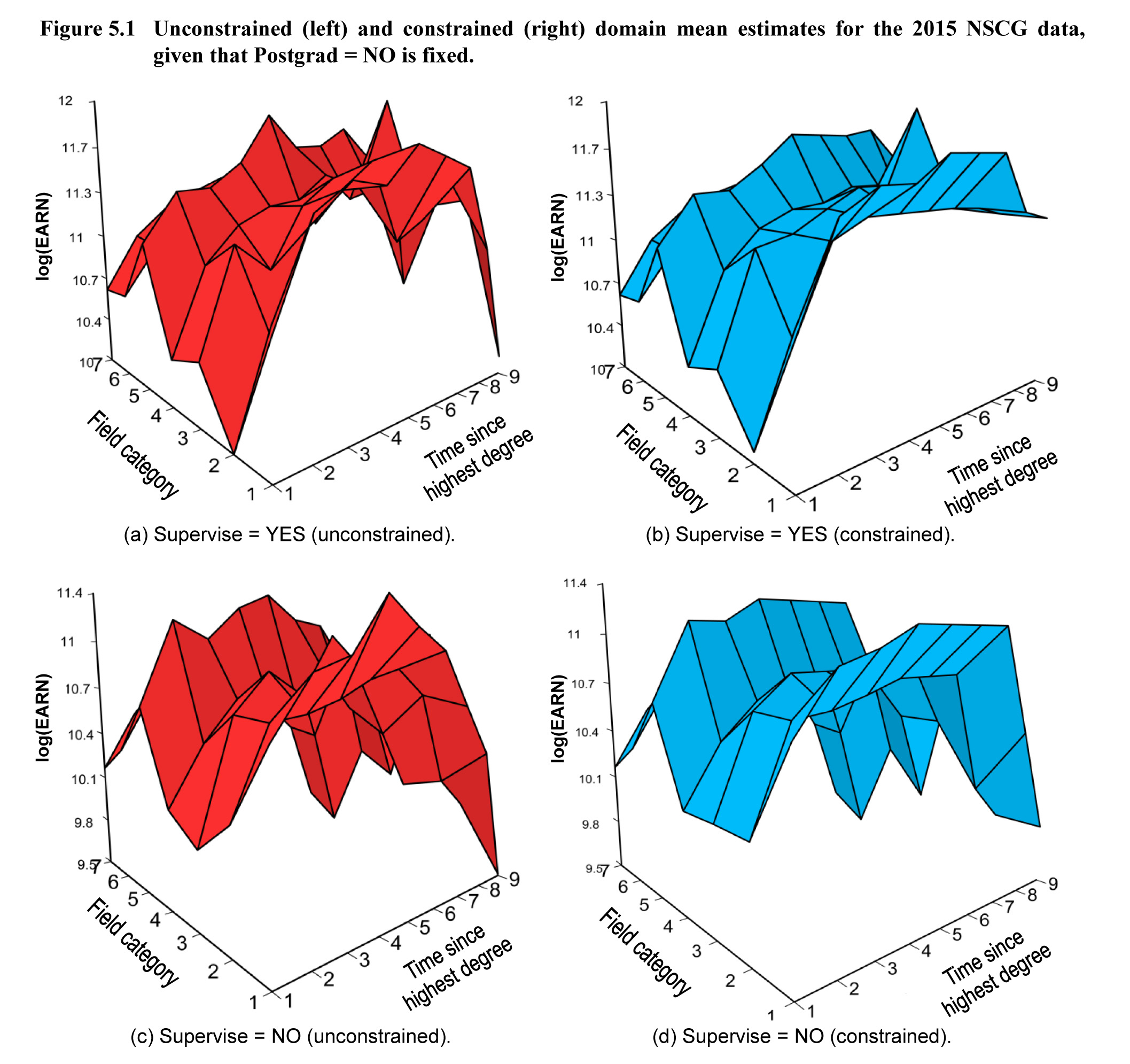
Description for Figure 5.1
Figure presenting four three-dimensional graphs of the domain mean estimates for the 2015 NSCG data, given that Postgrad = NO is fixed. The first two graphs show the constrained and unconstrained estimators given that Supervise = YES. For both graphs, log(EARN) is on the vertical axis, ranging from 10 to 12. The field category, ranging from 1 to 7, and the time since highest degree, ranging from 1 to 9 are the horizontal axis. They cross at 1. The vertical axis crosses the field category at log(EARN) = 10 and field category = 7. The last two graphs show the constrained and unconstrained estimators given that Supervise = NO. For both graphs, log(EARN) is on the vertical axis, ranging from 9.5 to 11.4. The field category, ranging from 1 to 7, and the time since highest degree, ranging from 1 to 9 are the horizontal axis. They cross at 1. The vertical axis crosses the field category at log(EARN) = 9.5 and field category = 7. In both cases, the constrained estimator has a smoother behavior than the unconstrained.
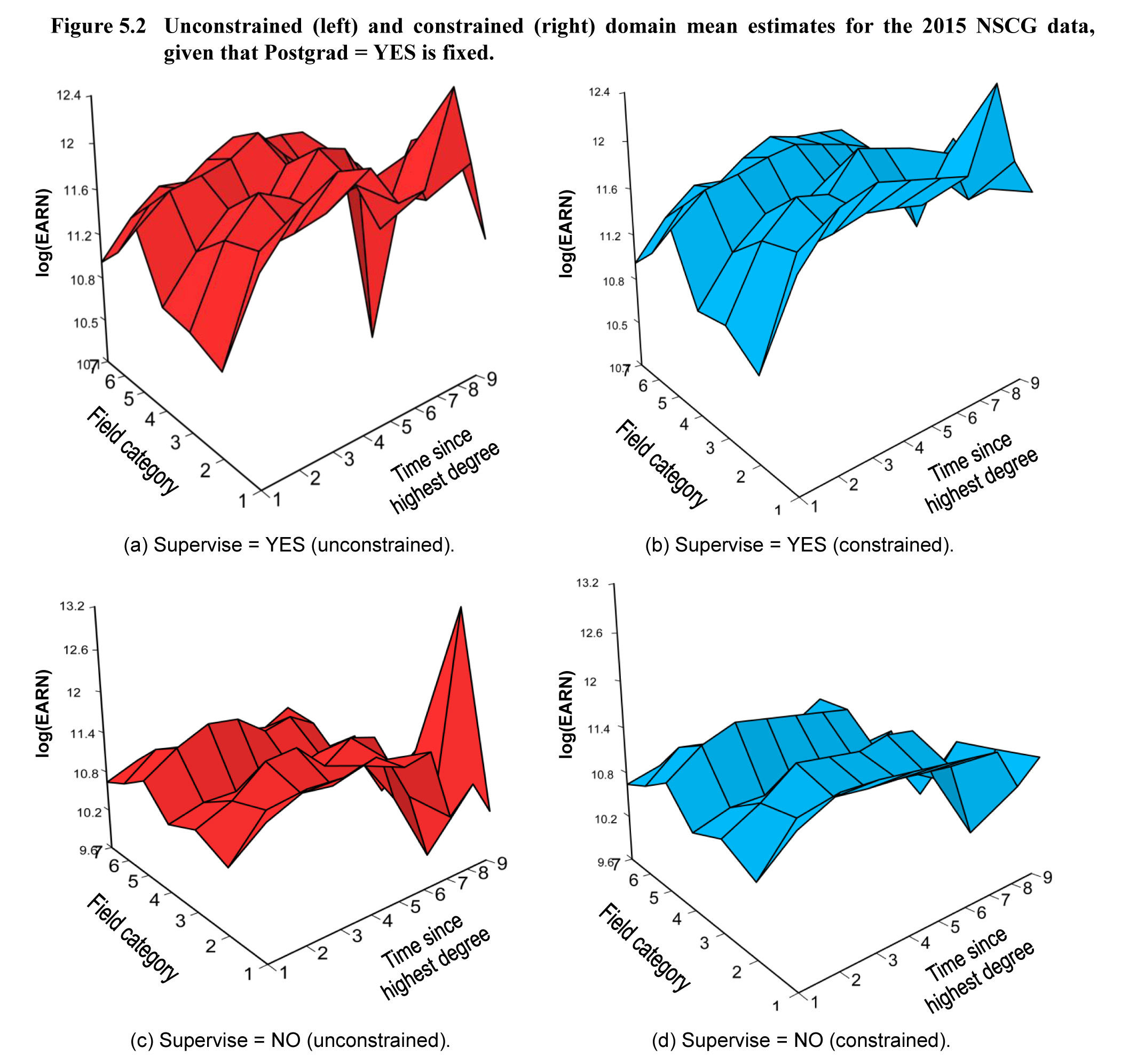
Description for Figure 5.2
Figure presenting four three-dimensional graphs of the domain mean estimates for the 2015 NSCG data, given that Postgrad = YES is fixed. The first two graphs show the constrained and unconstrained estimators given that Supervise = YES. For both graphs, log(EARN) is on the vertical axis, ranging from 10.1 to 12.4. The field category, ranging from 1 to 7, and the time since highest degree, ranging from 1 to 9 are the horizontal axis. They cross at 1. The vertical axis crosses the field category at log(EARN) = 10.1 and field category = 7. The last two graphs show the constrained and unconstrained estimators given that Supervise = NO. For both graphs, log(EARN) is on the vertical axis, ranging from 9.6 to 13.2. The field category, ranging from 1 to 7, and the time since highest degree, ranging from 1 to 9 are the horizontal axis. They cross at 1. The vertical axis crosses the field category at log(EARN) = 9.6 and field category = 7.The unconstrained estimator has spikes that are corrected by the constrained estimator which is smoother.
Standard errors for both unconstrained and constrained estimates are computed using the 2015 NSCG replicate weights, which are based on successive difference replication method (Opsomer, Breidt, White and Li, 2016). The replicate weights and adjustment factors were provided by the Program Director of the Human Resources Statistics Program from the NCSES and are available upon request.
Figure 5.3 displays the ratio of these estimates for each of the 252 domains. In the vast majority of cases, the standard error estimates of the proposed estimator are lower than those for the unconstrained estimator, with improvements of as much as 7 times smaller. However, there are some cases where the opposite behavior occurs. These are investigated in Figure 5.4, which shows plots of two different domain “slices”: one with respect to the Time since highest degree variable and other with respect to Field category. These plots include unconstrained and constrained estimates, Wald confidence intervals and sample sizes. Each of these two slices contain one of the two domains that can be easily identified in Figure 5.3 to have the smallest ratios.
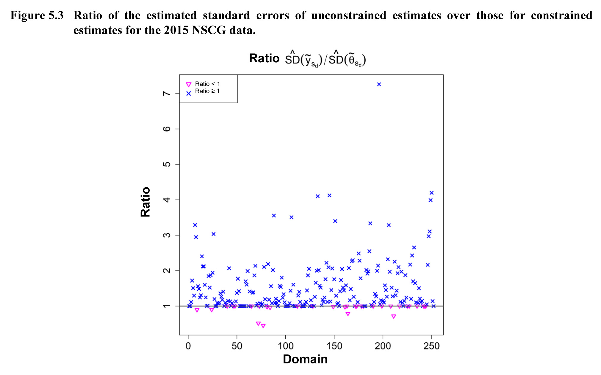
Description for Figure 5.3
Scatter plot of the ratios of the estimated standard errors of unconstrained estimates over those for constrained estimates for the 2015 NSCG data. Ratios ranging from 1 to 7 is on the y axis. Domains ranging from 0 to 250 are on the x axis. In the vast majority of cases, the standard error estimates of the proposed estimator are lower than those for the unconstrained estimator, with improvements of as much as 7 times smaller. However, there are some cases where the opposite behavior occurs.
The first of these domains is displayed in Figure 5.4(a) and 5.4(c), indexed by 5. The unconstrained estimates for the domains indexed by 5 and 6 violate the monotonicity assumption, and thus, are being pooled to obtain the constrained estimates (additional pooling with domains in other “slices” is also occurring, but not visible in this plot). As can be seen in Figure 5.4(a), the confidence interval is narrower for the unconstrained estimates. However, the estimated standard error of the unconstrained estimator of domain 6 is very large, and pooling with domain 5 greatly stabilizes both the estimator and the estimated standard errors for that domain. Figure 5.4(c) shows that the samples sizes on these domains are reasonably large at approximately 100 observations each, implying that the noticed monotonicity violation might be in fact true in the population. The final decision on the balance between the improved stability of some domains with the potential for bias due to incorrect constraints would need to be carefully evaluated.
The second domain where unconstrained estimates produce smaller standard deviation estimates is displayed in Figure 5.4(b) and 5.4(d), indexed by 1. Here, this domain is being pooled with its neighboring domain to obtain the constrained estimate. However, as these two domains have very low sample sizes, the unconstrained estimates might be considered as unreliable, so that their estimated standard errors are not a good indication of their precision. The constrained estimator appears to be preferred here because of the increase in the effective cell size.
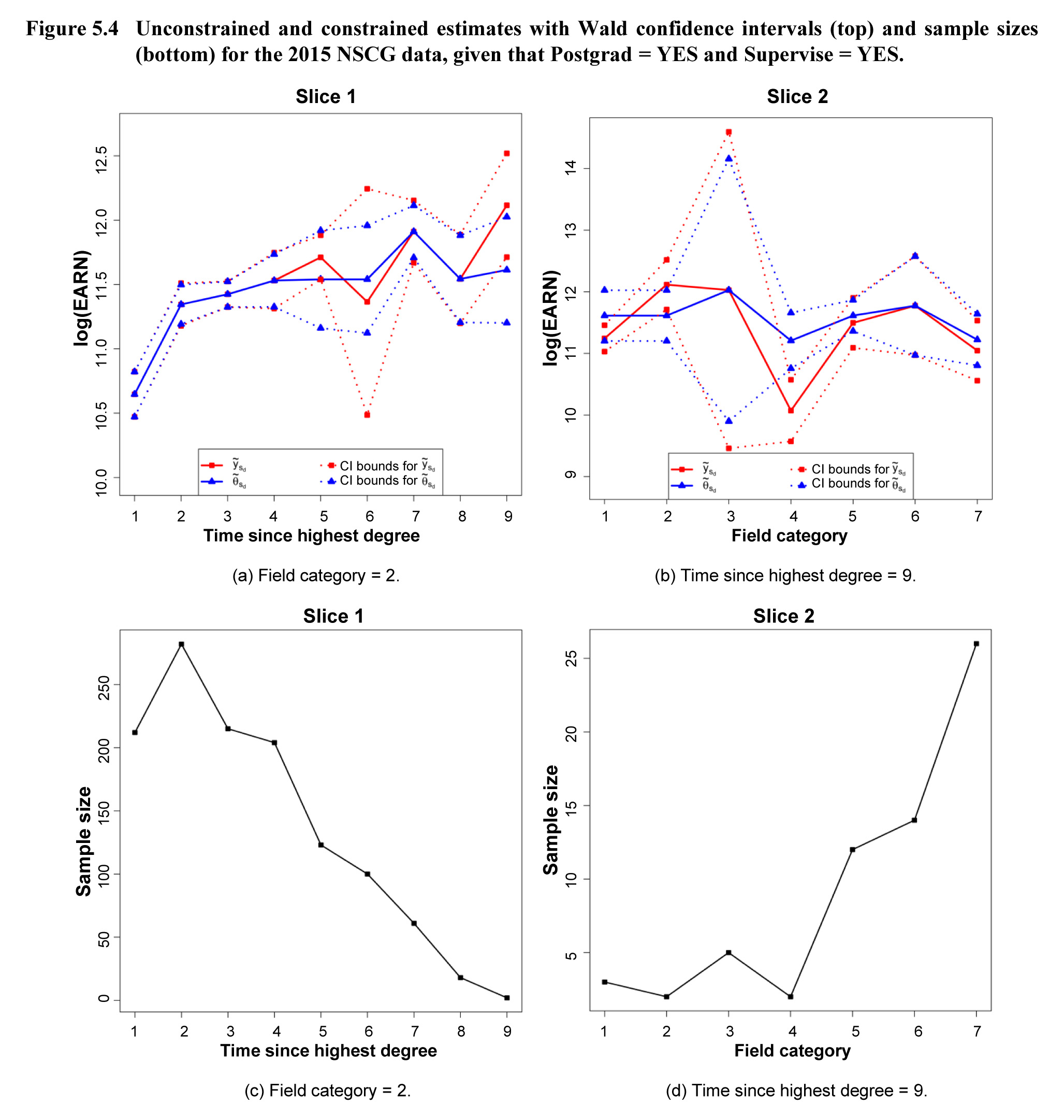
Description for Figure 5.4
Figure presenting four graphs. For slice 1, where field category = 2, the first graph includes unconstrained and constrained estimates with their Wald confidence intervals. Log(EARN) is on the y axis, ranging from 10 to 12.5. The time since highest degree ranging from 1 to 9 is on the x axis. The confidence interval is narrower for the unconstrained estimates. However, the estimated standard error of the unconstrained estimator of domain 6 is very large, and pooling with domain 5 greatly stabilizes both the estimator and the estimated standard errors for that domain.The second graph for slice 1 shows the sample size on the y axis, ranging from 0 to 250 vs the time since highest degree ranging from 1 to 9. The samples sizes on these domains are reasonably large at approximately 100 observations each, implying that the noticed monotonicity violation might be in fact true in the population.
For slice 2, where time since highest degree = 9, the first graph includes unconstrained and constrained estimates with their Wald confidence intervals. Log(EARN) is on the y axis, ranging from 9 to 14. The field category ranging from 1 to 7 is on the x axis. The confidence interval is narrower for the unconstrained estimates. The second graph for slice 2 shows the sample size on the y axis, ranging from 5 to 25 vs the field category ranging from 1 to 7. The samples sizes are smaller.
- Date modified: