Small area estimation methods under cut-off sampling
Section 9. Estimation of total sales in Spanish provinces

Here we describe an application to the estimation of the total sales of a certain tobacco product in the Spanish provinces. The available data set contains, for N = MathType@MTEF@5@5@+= feaagKart1ev2aqatCvAUfeBSjuyZL2yd9gzLbvyNv2CaerbuLwBLn hiov2DGi1BTfMBaeXatLxBI9gBaerbd9wDYLwzYbItLDharqqtubsr 4rNCHbGeaGqiFu0Je9sqqrpepC0xbbL8F4rqqrpgpC0xe9GqFf0xc9 qqpeuf0xe9q8qiYRWFGCk9vi=dbbf9v8Gq0db9qqpm0dXdHqpq0=vr 0=vr0=edbaqaaeGaciGaaiaabeqaamaabaabaaGcbaGaamOtaiaays W7caaI9aGaaGjcVdaa@3A61@ 12,791 tobacco establishments (practically all of them) in m = MathType@MTEF@5@5@+= feaagKart1ev2aqatCvAUfeBSjuyZL2yd9gzLbvyNv2CaerbuLwBLn hiov2DGi1BTfMBaeXatLxBI9gBaerbd9wDYLwzYbItLDharqqtubsr 4rNCHbGeaGqiFu0Je9sqqrpepC0xbbL8F4rqqrpgpC0xe9GqFf0xc9 qqpeuf0xe9q8qiYRWFGCk9vi=dbbf9v8Gq0db9qqpm0dXdHqpq0=vr 0=vr0=edbaqaaeGaciGaaiaabeqaamaabaabaaGcbaGaamyBaiaays W7caaI9aGaaGjcVdaa@3A80@ 48 provinces from Spain (the Canary Islands, Ceuta and Melilla are not included), the volume of purchases made by each establishment of this product during the three months previous to November 2016 ( z i j , MathType@MTEF@5@5@+= feaagKart1ev2aqatCvAUfeBSjuyZL2yd9gzLbvyNv2CaerbuLwBLn hiov2DGi1BTfMBaeXatLxBI9gBaerbd9wDYLwzYbItLDharqqtubsr 4rNCHbGeaGqiFu0Je9sqqrpepC0xbbL8F4rqqrpgpC0xe9GqFf0xc9 qqpeuf0xe9q8qiYRWFGCk9vi=dbbf9v8Gq0db9qqpm0dXdHqpq0=vr 0=vr0=edbaqaaeGaciGaaiaabeqaamaabaabaaGcbaGaaiikaiaadQ hadaWgaaWcbaGaamyAaiaadQgaaeqaaOGaaiilaaaa@3A17@ in euros). It also contains a variable indicating whether the establishment is supplied with a device recording all the required information about each sale. Only the establishments with larger sales are supplied with such a device. Those establishments (in total n = MathType@MTEF@5@5@+= feaagKart1ev2aqatCvAUfeBSjuyZL2yd9gzLbvyNv2CaerbuLwBLn hiov2DGi1BTfMBaeXatLxBI9gBaerbd9wDYLwzYbItLDharqqtubsr 4rNCHbGeaGqiFu0Je9sqqrpepC0xbbL8F4rqqrpgpC0xe9GqFf0xc9 qqpeuf0xe9q8qiYRWFGCk9vi=dbbf9v8Gq0db9qqpm0dXdHqpq0=vr 0=vr0=edbaqaaeGaciGaaiaabeqaamaabaabaaGcbaGaamOBaiaays W7caaI9aGaaGjcVdaa@3A81@ 1,842) are able to report proper data on sales and therefore the volume of sales ( v i j , MathType@MTEF@5@5@+= feaagKart1ev2aqatCvAUfeBSjuyZL2yd9gzLbvyNv2CaerbuLwBLn hiov2DGi1BTfMBaeXatLxBI9gBaerbd9wDYLwzYbItLDharqqtubsr 4rNCHbGeaGqiFu0Je9sqqrpepC0xbbL8F4rqqrpgpC0xe9GqFf0xc9 qqpeuf0xe9q8qiYRWFGCk9vi=dbbf9v8Gq0db9qqpm0dXdHqpq0=vr 0=vr0=edbaqaaeGaciGaaiaabeqaamaabaabaaGcbaGaaiikaiaadA hadaWgaaWcbaGaamyAaiaadQgaaeqaaOGaaiilaaaa@3A13@ in euros) of the considered product in November 2016 is also included in the data for those establishments.

We estimate the total sales V i = i = 1 N i v i j MathType@MTEF@5@5@+= feaagKart1ev2aqatCvAUfeBSjuyZL2yd9gzLbvyNv2CaerbuLwBLn hiov2DGi1BTfMBaeXatLxBI9gBaerbd9wDYLwzYbItLDharqqtubsr 4rNCHbGeaGqiFu0Je9sqqrpepC0xbbL8F4rqqrpgpC0xe9GqFf0xc9 qqpeuf0xe9q8qiYRWFGCk9vi=dbbf9v8Gq0db9qqpm0dXdHqpq0=vr 0=vr0=edbaqaaeGaciGaaiaabeqaamaabaabaaGcbaGaamOvamaaBa aaleaacaWGPbaabeaakiaaysW7caaI9aGaaGjbVpaaqadabeWcbaGa amyAaiaai2dacaaIXaaabaGaamOtamaaBaaameaacaWGPbaabeaaa0 GaeyyeIuoakiaaykW7caWG2bWaaSbaaSqaaiaadMgacaWGQbaabeaa aaa@4683@ in each of the m = MathType@MTEF@5@5@+= feaagKart1ev2aqatCvAUfeBSjuyZL2yd9gzLbvyNv2CaerbuLwBLn hiov2DGi1BTfMBaeXatLxBI9gBaerbd9wDYLwzYbItLDharqqtubsr 4rNCHbGeaGqiFu0Je9sqqrpepC0xbbL8F4rqqrpgpC0xe9GqFf0xc9 qqpeuf0xe9q8qiYRWFGCk9vi=dbbf9v8Gq0db9qqpm0dXdHqpq0=vr 0=vr0=edbaqaaeGaciGaaiaabeqaamaabaabaaGcbaGaamyBaiaays W7caaI9aGaaGjcVdaa@3A80@ 48 provinces included in the data using the basic direct, the selected calibration estimators and a model-based estimator. Establishments j MathType@MTEF@5@5@+= feaagKart1ev2aqatCvAUfeBSjuyZL2yd9gzLbvyNv2CaerbuLwBLn hiov2DGi1BTfMBaeXatLxBI9gBaerbd9wDYLwzYbItLDharqqtubsr 4rNCHbGeaGqiFu0Je9sqqrpepC0xbbL8F4rqqrpgpC0xe9GqFf0xc9 qqpeuf0xe9q8qiYRWFGCk9vi=dbbf9v8Gq0db9qqpm0dXdHqpq0=vr 0=vr0=edbaqaaeGaciGaaiaabeqaamaabaabaaGcbaGaamOAaaaa@3698@ with both z i j MathType@MTEF@5@5@+= feaagKart1ev2aqatCvAUfeBSjuyZL2yd9gzLbvyNv2CaerbuLwBLn hiov2DGi1BTfMBaeXatLxBI9gBaerbd9wDYLwzYbItLDharqqtubsr 4rNCHbGeaGqiFu0Je9sqqrpepC0xbbL8F4rqqrpgpC0xe9GqFf0xc9 qqpeuf0xe9q8qiYRWFGCk9vi=dbbf9v8Gq0db9qqpm0dXdHqpq0=vr 0=vr0=edbaqaaeGaciGaaiaabeqaamaabaabaaGcbaGaamOEamaaBa aaleaacaWGPbGaamOAaaqabaaaaa@38B1@ and v i j MathType@MTEF@5@5@+= feaagKart1ev2aqatCvAUfeBSjuyZL2yd9gzLbvyNv2CaerbuLwBLn hiov2DGi1BTfMBaeXatLxBI9gBaerbd9wDYLwzYbItLDharqqtubsr 4rNCHbGeaGqiFu0Je9sqqrpepC0xbbL8F4rqqrpgpC0xe9GqFf0xc9 qqpeuf0xe9q8qiYRWFGCk9vi=dbbf9v8Gq0db9qqpm0dXdHqpq0=vr 0=vr0=edbaqaaeGaciGaaiaabeqaamaabaabaaGcbaGaamODamaaBa aaleaacaWGPbGaamOAaaqabaaaaa@38AD@ available for a province i MathType@MTEF@5@5@+= feaagKart1ev2aqatCvAUfeBSjuyZL2yd9gzLbvyNv2CaerbuLwBLn hiov2DGi1BTfMBaeXatLxBI9gBaerbd9wDYLwzYbItLDharqqtubsr 4rNCHbGeaGqiFu0Je9sqqrpepC0xbbL8F4rqqrpgpC0xe9GqFf0xc9 qqpeuf0xe9q8qiYRWFGCk9vi=dbbf9v8Gq0db9qqpm0dXdHqpq0=vr 0=vr0=edbaqaaeGaciGaaiaabeqaamaabaabaaGcbaGaamyAaaaa@3697@ compose the set of included units U i I , MathType@MTEF@5@5@+= feaagKart1ev2aqatCvAUfeBSjuyZL2yd9gzLbvyNv2CaerbuLwBLn hiov2DGi1BTfMBaeXatLxBI9gBaerbd9wDYLwzYbItLDharqqtubsr 4rNCHbGeaGqiFu0Je9sqqrpepC0xbbL8F4rqqrpgpC0xe9GqFf0xc9 qqpeuf0xe9q8qiYRWFGCk9vi=dbbf9v8Gq0db9qqpm0dXdHqpq0=vr 0=vr0=edbaqaaeGaciGaaiaabeqaamaabaabaaGcbaGaamyvamaaBa aaleaacaWGPbGaamysaaqabaGccaGGSaaaaa@3925@ which equals the sample s i MathType@MTEF@5@5@+= feaagKart1ev2aqatCvAUfeBSjuyZL2yd9gzLbvyNv2CaerbuLwBLn hiov2DGi1BTfMBaeXatLxBI9gBaerbd9wDYLwzYbItLDharqqtubsr 4rNCHbGeaGqiFu0Je9sqqrpepC0xbbL8F4rqqrpgpC0xe9GqFf0xc9 qqpeuf0xe9q8qiYRWFGCk9vi=dbbf9v8Gq0db9qqpm0dXdHqpq0=vr 0=vr0=edbaqaaeGaciGaaiaabeqaamaabaabaaGcbaGaam4CamaaBa aaleaacaWGPbaabeaaaaa@37BB@ in this case (there is no sampling within U i I ) . MathType@MTEF@5@5@+= feaagKart1ev2aqatCvAUfeBSjuyZL2yd9gzLbvyNv2CaerbuLwBLn hiov2DGi1BTfMBaeXatLxBI9gBaerbd9wDYLwzYbItLDharqqtubsr 4rNCHbGeaGqiFu0Je9sqqrpepC0xbbL8F4rqqrpgpC0xe9GqFf0xc9 qqpeuf0xe9q8qiYRWFGCk9vi=dbbf9v8Gq0db9qqpm0dXdHqpq0=vr 0=vr0=edbaqaaeGaciGaaiaabeqaamaabaabaaGcbaGaamyvamaaBa aaleaacaWGPbGaamysaaqabaGccaGGPaGaaiOlaaaa@39D4@ Then, here the basic direct estimators are given by V ^ i HA = N i V ¯ i I , MathType@MTEF@5@5@+= feaagKart1ev2aqatCvAUfeBSjuyZL2yd9gzLbvyNv2CaerbuLwBLn hiov2DGi1BTfMBaeXatLxBI9gBaerbd9wDYLwzYbItLDharqqtubsr 4rNCHbGeaGqiFu0Je9sqqrpepC0xbbL8F4rqqrpgpC0xe9GqFf0xc9 qqpeuf0xe9q8qiYRWFGCk9vi=dbbf9v8Gq0db9qqpm0dXdHqpq0=vr 0=vr0=edbaqaaeGaciGaaiaabeqaamaabaabaaGcbaGabmOvayaaja Waa0baaSqaaiaadMgaaeaacaqGibGaaeyqaaaakiaaysW7caaI9aGa aGjbVlaad6eadaWgaaWcbaGaamyAaaqabaGcceWGwbGbaebadaWgaa WcbaGaamyAaiaadMeaaeqaaOGaaiilaaaa@42B5@ i = 1, , m , MathType@MTEF@5@5@+= feaagKart1ev2aqatCvAUfeBSjuyZL2yd9gzLbvyNv2CaerbuLwBLn hiov2DGi1BTfMBaeXatLxBI9gBaerbd9wDYLwzYbItLDharqqtubsr 4rNCHbGeaGqiFu0Je9sqqrpepC0xbbL8F4rqqrpgpC0xe9GqFf0xc9 qqpeuf0xe9q8qiYRWFGCk9vi=dbbf9v8Gq0db9qqpm0dXdHqpq0=vr 0=vr0=edbaqaaeGaciGaaiaabeqaamaabaabaaGcbaGaamyAaiaays W7caaI9aGaaGjbVlaaigdacaaISaGaaGjbVlablAciljaaiYcacaaM e8UaamyBaiaacYcaaaa@427D@ which have actually zero variance, but might be severely biased. Since true values in real applications are not available and therefore real biases cannot be evaluated (there is no information from U i E ) , MathType@MTEF@5@5@+= feaagKart1ev2aqatCvAUfeBSjuyZL2yd9gzLbvyNv2CaerbuLwBLn hiov2DGi1BTfMBaeXatLxBI9gBaerbd9wDYLwzYbItLDharqqtubsr 4rNCHbGeaGqiFu0Je9sqqrpepC0xbbL8F4rqqrpgpC0xe9GqFf0xc9 qqpeuf0xe9q8qiYRWFGCk9vi=dbbf9v8Gq0db9qqpm0dXdHqpq0=vr 0=vr0=edbaqaaeGaciGaaiaabeqaamaabaabaaGcbaGaamyvamaaBa aaleaacaWGPbGaamyraaqabaGccaGGPaGaaiilaaaa@39CE@ here we will compare the estimators considering the set of establishments with sales recorded from each province as a SRSWOR from that province. Note that this is the best scenario for the basic direct estimator. Thus, for the basic direct estimator V ^ i HA MathType@MTEF@5@5@+= feaagKart1ev2aqatCvAUfeBSjuyZL2yd9gzLbvyNv2CaerbuLwBLn hiov2DGi1BTfMBaeXatLxBI9gBaerbd9wDYLwzYbItLDharqqtubsr 4rNCHbGeaGqiFu0Je9sqqrpepC0xbbL8F4rqqrpgpC0xe9GqFf0xc9 qqpeuf0xe9q8qiYRWFGCk9vi=dbbf9v8Gq0db9qqpm0dXdHqpq0=vr 0=vr0=edbaqaaeGaciGaaiaabeqaamaabaabaaGcbaGabmOvayaaja Waa0baaSqaaiaadMgaaeaacaqGibGaaeyqaaaaaaa@393E@ considering that the actual sample s i = U i I MathType@MTEF@5@5@+= feaagKart1ev2aqatCvAUfeBSjuyZL2yd9gzLbvyNv2CaerbuLwBLn hiov2DGi1BTfMBaeXatLxBI9gBaerbd9wDYLwzYbItLDharqqtubsr 4rNCHbGeaGqiFu0Je9sqqrpepC0xbbL8F4rqqrpgpC0xe9GqFf0xc9 qqpeuf0xe9q8qiYRWFGCk9vi=dbbf9v8Gq0db9qqpm0dXdHqpq0=vr 0=vr0=edbaqaaeGaciGaaiaabeqaamaabaabaaGcbaGaam4CamaaBa aaleaacaWGPbaabeaakiaaysW7caaI9aGaaGjbVlaadwfadaWgaaWc baGaamyAaiaadMeaaeqaaaaa@3E68@ is a SRSWOR from U i , MathType@MTEF@5@5@+= feaagKart1ev2aqatCvAUfeBSjuyZL2yd9gzLbvyNv2CaerbuLwBLn hiov2DGi1BTfMBaeXatLxBI9gBaerbd9wDYLwzYbItLDharqqtubsr 4rNCHbGeaGqiFu0Je9sqqrpepC0xbbL8F4rqqrpgpC0xe9GqFf0xc9 qqpeuf0xe9q8qiYRWFGCk9vi=dbbf9v8Gq0db9qqpm0dXdHqpq0=vr 0=vr0=edbaqaaeGaciGaaiaabeqaamaabaabaaGcbaGaamyvamaaBa aaleaacaWGPbaabeaakiaacYcaaaa@3857@ the variance equals the MSE (we ignore the bias). A design-unbiased estimator of the MSE is then

mse π ( V ^ i ) = N i 2 s i 2 n i ( 1 n i N i ) , i = 1, , m , MathType@MTEF@5@5@+= feaagKart1ev2aaatCvAUfeBSjuyZL2yd9gzLbvyNv2CaerbuLwBLn hiov2DGi1BTfMBaeXatLxBI9gBaerbd9wDYLwzYbItLDharqqtubsr 4rNCHbGeaGqiFu0Je9sqqrpepC0xbbL8F4rqqrpgpC0xe9GqFf0xc9 qqpeuf0xe9q8qiYRWFGCk9vi=dbbf9v8Gq0db9qqpm0dXdHqpq0=vr 0=vr0=edbaqaaeGaciGaaiaabeqaamaabaabaaGcbaGaaeyBaiaabo hacaqGLbWaaSbaaSqaaiabec8aWbqabaGcdaqadeqaaiqadAfagaqc amaaBaaaleaacaWGPbaabeaaaOGaayjkaiaawMcaaiaaysW7caaI9a GaaGjbVlaad6eadaqhaaWcbaGaamyAaaqaaiaaikdaaaGccaaMc8+a aSaaaeaacaWGZbWaa0baaSqaaiaadMgaaeaacaaIYaaaaaGcbaGaam OBamaaBaaaleaacaWGPbaabeaaaaGccaaMc8+aaeWaaeaacaaIXaGa aGjbVlabgkHiTiaaysW7daWcaaqaaiaad6gadaWgaaWcbaGaamyAaa qabaaakeaacaWGobWaaSbaaSqaaiaadMgaaeqaaaaaaOGaayjkaiaa wMcaaiaaiYcacaaMf8UaamyAaiaaysW7caaI9aGaaGjbVlaaigdaca aISaGaaGjbVlablAciljaaiYcacaaMe8UaamyBaiaaiYcaaaa@6634@

where s i 2 = ( n i 1 ) 1 j s i ( v i j v ¯ i s ) 2 MathType@MTEF@5@5@+= feaagKart1ev2aqatCvAUfeBSjuyZL2yd9gzLbvyNv2CaerbuLwBLn hiov2DGi1BTfMBaeXatLxBI9gBaerbd9wDYLwzYbItLDharqqtubsr 4rNCHbGeaGqiFu0Je9sqqrpepC0xbbL8F4rqqrpgpC0xe9GqFf0xc9 qqpeuf0xe9q8qiYRWFGCk9vi=dbbf9v8Gq0db9qqpm0dXdHqpq0=vr 0=vr0=edbaqaaeGaciGaaiaabeqaamaabaabaaGcbaGaam4CamaaDa aaleaacaWGPbaabaGaaGOmaaaakiaaysW7caaI9aGaaGjbVpaabmqa baGaamOBamaaBaaaleaacaWGPbaabeaakiabgkHiTiaaigdaaiaawI cacaGLPaaadaahaaWcbeqaaiabgkHiTiaaigdaaaGcdaaeqaqabSqa aiaadQgacqGHiiIZcaWGZbWaaSbaaWqaaiaadMgaaeqaaaWcbeqdcq GHris5aOGaaGPaVpaabmqabaGaamODamaaBaaaleaacaWGPbGaamOA aaqabaGccaaMe8UaeyOeI0IaaGjbVlqadAhagaqeamaaBaaaleaaca WGPbGaam4CaaqabaaakiaawIcacaGLPaaadaahaaWcbeqaaiaaikda aaaaaa@584C@ is the sample variance of the sales for province i MathType@MTEF@5@5@+= feaagKart1ev2aqatCvAUfeBSjuyZL2yd9gzLbvyNv2CaerbuLwBLn hiov2DGi1BTfMBaeXatLxBI9gBaerbd9wDYLwzYbItLDharqqtubsr 4rNCHbGeaGqiFu0Je9sqqrpepC0xbbL8F4rqqrpgpC0xe9GqFf0xc9 qqpeuf0xe9q8qiYRWFGCk9vi=dbbf9v8Gq0db9qqpm0dXdHqpq0=vr 0=vr0=edbaqaaeGaciGaaiaabeqaamaabaabaaGcbaGaamyAaaaa@3697@ and here n i = N i I , MathType@MTEF@5@5@+= feaagKart1ev2aqatCvAUfeBSjuyZL2yd9gzLbvyNv2CaerbuLwBLn hiov2DGi1BTfMBaeXatLxBI9gBaerbd9wDYLwzYbItLDharqqtubsr 4rNCHbGeaGqiFu0Je9sqqrpepC0xbbL8F4rqqrpgpC0xe9GqFf0xc9 qqpeuf0xe9q8qiYRWFGCk9vi=dbbf9v8Gq0db9qqpm0dXdHqpq0=vr 0=vr0=edbaqaaeGaciGaaiaabeqaamaabaabaaGcbaGaamOBamaaBa aaleaacaWGPbaabeaakiaaysW7caaI9aGaaGjbVlaad6eadaWgaaWc baGaamyAaiaadMeaaeqaaOGaaiilaaaa@3F16@ i = 1, , m . MathType@MTEF@5@5@+= feaagKart1ev2aqatCvAUfeBSjuyZL2yd9gzLbvyNv2CaerbuLwBLn hiov2DGi1BTfMBaeXatLxBI9gBaerbd9wDYLwzYbItLDharqqtubsr 4rNCHbGeaGqiFu0Je9sqqrpepC0xbbL8F4rqqrpgpC0xe9GqFf0xc9 qqpeuf0xe9q8qiYRWFGCk9vi=dbbf9v8Gq0db9qqpm0dXdHqpq0=vr 0=vr0=edbaqaaeGaciGaaiaabeqaamaabaabaaGcbaGaamyAaiaays W7caaI9aGaaGjbVlaaigdacaaISaGaaGjbVlablAciljaaiYcacaaM e8UaamyBaiaac6caaaa@427F@

For the estimators that consider a regression model, we first make a preliminary descriptive analysis of the variables. Histograms of sales v i j MathType@MTEF@5@5@+= feaagKart1ev2aqatCvAUfeBSjuyZL2yd9gzLbvyNv2CaerbuLwBLn hiov2DGi1BTfMBaeXatLxBI9gBaerbd9wDYLwzYbItLDharqqtubsr 4rNCHbGeaGqiFu0Je9sqqrpepC0xbbL8F4rqqrpgpC0xe9GqFf0xc9 qqpeuf0xe9q8qiYRWFGCk9vi=dbbf9v8Gq0db9qqpm0dXdHqpq0=vr 0=vr0=edbaqaaeGaciGaaiaabeqaamaabaabaaGcbaGaamODamaaBa aaleaacaWGPbGaamOAaaqabaaaaa@38AD@ and of purchases z i j MathType@MTEF@5@5@+= feaagKart1ev2aqatCvAUfeBSjuyZL2yd9gzLbvyNv2CaerbuLwBLn hiov2DGi1BTfMBaeXatLxBI9gBaerbd9wDYLwzYbItLDharqqtubsr 4rNCHbGeaGqiFu0Je9sqqrpepC0xbbL8F4rqqrpgpC0xe9GqFf0xc9 qqpeuf0xe9q8qiYRWFGCk9vi=dbbf9v8Gq0db9qqpm0dXdHqpq0=vr 0=vr0=edbaqaaeGaciGaaiaabeqaamaabaabaaGcbaGaamOEamaaBa aaleaacaWGPbGaamOAaaqabaaaaa@38B1@ show right-skewed distributions for both variables. Moreover, a scatterplot of ordinary LS residuals from a linear model for v i j MathType@MTEF@5@5@+= feaagKart1ev2aqatCvAUfeBSjuyZL2yd9gzLbvyNv2CaerbuLwBLn hiov2DGi1BTfMBaeXatLxBI9gBaerbd9wDYLwzYbItLDharqqtubsr 4rNCHbGeaGqiFu0Je9sqqrpepC0xbbL8F4rqqrpgpC0xe9GqFf0xc9 qqpeuf0xe9q8qiYRWFGCk9vi=dbbf9v8Gq0db9qqpm0dXdHqpq0=vr 0=vr0=edbaqaaeGaciGaaiaabeqaamaabaabaaGcbaGaamODamaaBa aaleaacaWGPbGaamOAaaqabaaaaa@38AD@ in terms of z i j , MathType@MTEF@5@5@+= feaagKart1ev2aqatCvAUfeBSjuyZL2yd9gzLbvyNv2CaerbuLwBLn hiov2DGi1BTfMBaeXatLxBI9gBaerbd9wDYLwzYbItLDharqqtubsr 4rNCHbGeaGqiFu0Je9sqqrpepC0xbbL8F4rqqrpgpC0xe9GqFf0xc9 qqpeuf0xe9q8qiYRWFGCk9vi=dbbf9v8Gq0db9qqpm0dXdHqpq0=vr 0=vr0=edbaqaaeGaciGaaiaabeqaamaabaabaaGcbaGaamOEamaaBa aaleaacaWGPbGaamOAaaqabaGccaGGSaaaaa@396B@ against z i j MathType@MTEF@5@5@+= feaagKart1ev2aqatCvAUfeBSjuyZL2yd9gzLbvyNv2CaerbuLwBLn hiov2DGi1BTfMBaeXatLxBI9gBaerbd9wDYLwzYbItLDharqqtubsr 4rNCHbGeaGqiFu0Je9sqqrpepC0xbbL8F4rqqrpgpC0xe9GqFf0xc9 qqpeuf0xe9q8qiYRWFGCk9vi=dbbf9v8Gq0db9qqpm0dXdHqpq0=vr 0=vr0=edbaqaaeGaciGaaiaabeqaamaabaabaaGcbaGaamOEamaaBa aaleaacaWGPbGaamOAaaqabaaaaa@38B1@ reveals a mild pattern of heteroscedasticity. Transforming the sales with the squared root, that is, taking y i j = v i j 1 / 2 MathType@MTEF@5@5@+= feaagKart1ev2aqatCvAUfeBSjuyZL2yd9gzLbvyNv2CaerbuLwBLn hiov2DGi1BTfMBaeXatLxBI9gBaerbd9wDYLwzYbItLDharqqtubsr 4rNCHbGeaGqiFu0Je9sqqrpepC0xbbL8F4rqqrpgpC0xe9GqFf0xc9 qqpeuf0xe9q8qiYRWFGCk9vi=dbbf9v8Gq0db9qqpm0dXdHqpq0=vr 0=vr0=edbaqaaeGaciGaaiaabeqaamaabaabaaGcbaGaamyEamaaBa aaleaacaWGPbGaamOAaaqabaGccaaMe8UaaGypaiaaysW7caWG2bWa a0baaSqaaiaadMgacaWGQbaabaWaaSGbaeaacaaIXaaabaGaaGOmaa aaaaaaaa@412D@ as response variable and x i j = ( 1, x i j ) , MathType@MTEF@5@5@+= feaagKart1ev2aqatCvAUfeBSjuyZL2yd9gzLbvyNv2CaerbuLwBLn hiov2DGi1BTfMBaeXatLxBI9gBaerbd9wDYLwzYbItLDharqqtubsr 4rNCHbGeaGqiFu0Je9sqqrpepC0xbbL8F4rqqrpgpC0xe9GqFf0xc9 qqpeuf0xe9q8qiYRWFGCk9vi=dbbf9v8Gq0db9qqpm0dXdHqpq0=vr 0=vr0=edbaqaaeGaciGaaiaabeqaamaabaabaaGcbaGaaCiEamaaBa aaleaacaWGPbGaamOAaaqabaGccaaMe8UaaGypaiaaysW7daqadeqa aiaaigdacaaISaGaaGjbVlaadIhadaWgaaWcbaGaamyAaiaadQgaae qaaaGccaGLOaGaayzkaaWaaWbaaSqabeaajugybiadaITHYaIOaaGc caGGSaaaaa@48CC@ with x i j = z i j 1 / 2 MathType@MTEF@5@5@+= feaagKart1ev2aqatCvAUfeBSjuyZL2yd9gzLbvyNv2CaerbuLwBLn hiov2DGi1BTfMBaeXatLxBI9gBaerbd9wDYLwzYbItLDharqqtubsr 4rNCHbGeaGqiFu0Je9sqqrpepC0xbbL8F4rqqrpgpC0xe9GqFf0xc9 qqpeuf0xe9q8qiYRWFGCk9vi=dbbf9v8Gq0db9qqpm0dXdHqpq0=vr 0=vr0=edbaqaaeGaciGaaiaabeqaamaabaabaaGcbaGaamiEamaaBa aaleaacaWGPbGaamOAaaqabaGccaaMe8UaaGypaiaaysW7caWG6bWa a0baaSqaaiaadMgacaWGQbaabaWaaSGbaeaacaaIXaaabaGaaGOmaa aaaaaaaa@4130@ as covariate seems to minimize the problem. Accordingly, we will consider a nested error model (5.1) for the transformed sales y i j MathType@MTEF@5@5@+= feaagKart1ev2aqatCvAUfeBSjuyZL2yd9gzLbvyNv2CaerbuLwBLn hiov2DGi1BTfMBaeXatLxBI9gBaerbd9wDYLwzYbItLDharqqtubsr 4rNCHbGeaGqiFu0Je9sqqrpepC0xbbL8F4rqqrpgpC0xe9GqFf0xc9 qqpeuf0xe9q8qiYRWFGCk9vi=dbbf9v8Gq0db9qqpm0dXdHqpq0=vr 0=vr0=edbaqaaeGaciGaaiaabeqaamaabaabaaGcbaGaamyEamaaBa aaleaacaWGPbGaamOAaaqabaaaaa@38B0@ in terms of the transformed purchases x i j , MathType@MTEF@5@5@+= feaagKart1ev2aqatCvAUfeBSjuyZL2yd9gzLbvyNv2CaerbuLwBLn hiov2DGi1BTfMBaeXatLxBI9gBaerbd9wDYLwzYbItLDharqqtubsr 4rNCHbGeaGqiFu0Je9sqqrpepC0xbbL8F4rqqrpgpC0xe9GqFf0xc9 qqpeuf0xe9q8qiYRWFGCk9vi=dbbf9v8Gq0db9qqpm0dXdHqpq0=vr 0=vr0=edbaqaaeGaciGaaiaabeqaamaabaabaaGcbaGaamiEamaaBa aaleaacaWGPbGaamOAaaqabaGccaGGSaaaaa@3969@ and EBPs of the total sales in each province, V i = j = 1 N i v i j , MathType@MTEF@5@5@+= feaagKart1ev2aqatCvAUfeBSjuyZL2yd9gzLbvyNv2CaerbuLwBLn hiov2DGi1BTfMBaeXatLxBI9gBaerbd9wDYLwzYbItLDharqqtubsr 4rNCHbGeaGqiFu0Je9sqqrpepC0xbbL8F4rqqrpgpC0xe9GqFf0xc9 qqpeuf0xe9q8qiYRWFGCk9vi=dbbf9v8Gq0db9qqpm0dXdHqpq0=vr 0=vr0=edbaqaaeGaciGaaiaabeqaamaabaabaaGcbaGaamOvamaaBa aaleaacaWGPbaabeaakiaaysW7caaI9aGaaGjbVpaaqadabeWcbaGa amOAaiaai2dacaaIXaaabaGaamOtamaaBaaameaacaWGPbaabeaaa0 GaeyyeIuoakiaaykW7caWG2bWaaSbaaSqaaiaadMgacaWGQbaabeaa kiaacYcaaaa@473E@ will be computed based on this model. Note that, in terms of the model responses y i j , MathType@MTEF@5@5@+= feaagKart1ev2aqatCvAUfeBSjuyZL2yd9gzLbvyNv2CaerbuLwBLn hiov2DGi1BTfMBaeXatLxBI9gBaerbd9wDYLwzYbItLDharqqtubsr 4rNCHbGeaGqiFu0Je9sqqrpepC0xbbL8F4rqqrpgpC0xe9GqFf0xc9 qqpeuf0xe9q8qiYRWFGCk9vi=dbbf9v8Gq0db9qqpm0dXdHqpq0=vr 0=vr0=edbaqaaeGaciGaaiaabeqaamaabaabaaGcbaGaamyEamaaBa aaleaacaWGPbGaamOAaaqabaGccaGGSaaaaa@396A@ the total sales are given by V i = j = 1 N i y i j 2 = h ( y i ) . MathType@MTEF@5@5@+= feaagKart1ev2aqatCvAUfeBSjuyZL2yd9gzLbvyNv2CaerbuLwBLn hiov2DGi1BTfMBaeXatLxBI9gBaerbd9wDYLwzYbItLDharqqtubsr 4rNCHbGeaGqiFu0Je9sqqrpepC0xbbL8F4rqqrpgpC0xe9GqFf0xc9 qqpeuf0xe9q8qiYRWFGCk9vi=dbbf9v8Gq0db9qqpm0dXdHqpq0=vr 0=vr0=edbaqaaeGaciGaaiaabeqaamaabaabaaGcbaGaamOvamaaBa aaleaacaWGPbaabeaakiaaysW7caaI9aGaaGjbVpaaqadabeWcbaGa amOAaiaai2dacaaIXaaabaGaamOtamaaBaaameaacaWGPbaabeaaa0 GaeyyeIuoakiaaykW7caWG5bWaa0baaSqaaiaadMgacaWGQbaabaGa aGOmaaaakiaaysW7caaI9aGaaGjbVlaadIgadaqadeqaaiaahMhada WgaaWcbaGaamyAaaqabaaakiaawIcacaGLPaaacaGGUaaaaa@507E@ Then, the EBP of V i = h ( y i ) MathType@MTEF@5@5@+= feaagKart1ev2aqatCvAUfeBSjuyZL2yd9gzLbvyNv2CaerbuLwBLn hiov2DGi1BTfMBaeXatLxBI9gBaerbd9wDYLwzYbItLDharqqtubsr 4rNCHbGeaGqiFu0Je9sqqrpepC0xbbL8F4rqqrpgpC0xe9GqFf0xc9 qqpeuf0xe9q8qiYRWFGCk9vi=dbbf9v8Gq0db9qqpm0dXdHqpq0=vr 0=vr0=edbaqaaeGaciGaaiaabeqaamaabaabaaGcbaGaamOvamaaBa aaleaacaWGPbaabeaakiaaysW7caaI9aGaaGjbVlaadIgadaqadeqa aiaahMhadaWgaaWcbaGaamyAaaqabaaakiaawIcacaGLPaaaaaa@4026@ is given by V ^ i EBP = E m 3 [ h ( y i ) | y i s ; θ ^ ] , MathType@MTEF@5@5@+= feaagKart1ev2aqatCvAUfeBSjuyZL2yd9gzLbvyNv2CaerbuLwBLn hiov2DGi1BTfMBaeXatLxBI9gBaerbd9wDYLwzYbItLDharqqtubsr 4rNCHbGeaGqiFu0Je9sqqrpepC0xbbL8F4rqqrpgpC0xe9GqFf0xc9 qqpeuf0xe9q8qiYRWFGCk9vi=dbbf9v8Gq0db9qqpm0dXdHqpq0=vr 0=vr0=edbaqaaeGaciGaaiaabeqaamaabaabaaGcbaGabmOvayaaja Waa0baaSqaaiaadMgaaeaacaqGfbGaaeOqaiaabcfaaaGccaaMe8Ua aGypaiaaysW7caWGfbWaaSbaaSqaaiaad2gadaWgaaadbaGaaG4maa qabaaaleqaaOWaamWabeaadaabceqaaiaadIgadaqadeqaaiaahMha daWgaaWcbaGaamyAaaqabaaakiaawIcacaGLPaaacaaMc8oacaGLiW oacaaMc8UaaCyEamaaBaaaleaacaWGPbGaam4CaaqabaGccaaI7aGa aGjbVlqahI7agaqcaaGaay5waiaaw2faaiaacYcaaaa@5392@ i = 1, , m , MathType@MTEF@5@5@+= feaagKart1ev2aqatCvAUfeBSjuyZL2yd9gzLbvyNv2CaerbuLwBLn hiov2DGi1BTfMBaeXatLxBI9gBaerbd9wDYLwzYbItLDharqqtubsr 4rNCHbGeaGqiFu0Je9sqqrpepC0xbbL8F4rqqrpgpC0xe9GqFf0xc9 qqpeuf0xe9q8qiYRWFGCk9vi=dbbf9v8Gq0db9qqpm0dXdHqpq0=vr 0=vr0=edbaqaaeGaciGaaiaabeqaamaabaabaaGcbaGaamyAaiaays W7caaI9aGaaGjbVlaaigdacaaISaGaaGjbVlablAciljaaiYcacaaM e8UaamyBaiaacYcaaaa@427D@ which can be calculated analytically or approximated by Monte Carlo simulation. We estimate the model MSE of the EBP using the parametric bootstrap described in Section 7 for H i = V i , MathType@MTEF@5@5@+= feaagKart1ev2aqatCvAUfeBSjuyZL2yd9gzLbvyNv2CaerbuLwBLn hiov2DGi1BTfMBaeXatLxBI9gBaerbd9wDYLwzYbItLDharqqtubsr 4rNCHbGeaGqiFu0Je9sqqrpepC0xbbL8F4rqqrpgpC0xe9GqFf0xc9 qqpeuf0xe9q8qiYRWFGCk9vi=dbbf9v8Gq0db9qqpm0dXdHqpq0=vr 0=vr0=edbaqaaeGaciGaaiaabeqaamaabaabaaGcbaGaamisamaaBa aaleaacaWGPbaabeaakiaaysW7caaI9aGaaGjbVlaadAfadaWgaaWc baGaamyAaaqabaGccaGGSaaaaa@3E2A@ taking H i *(b) = V i *(b) MathType@MTEF@5@5@+= feaagKart1ev2aaatCvAUfeBSjuyZL2yd9gzLbvyNv2CaerbuLwBLn hiov2DGi1BTfMBaeXatLxBI9gBaerbd9wDYLwzYbItLDharqqtubsr 4rNCHbGeaGqiVu0Je9sqqrpepC0xbbL8F4rqqrFfpeea0xe9Lq=Jc9 vqaqpepm0xbba9pwe9Q8fs0=yqaqpepae9pg0FirpepeKkFr0xfr=x fr=xb9adbaqaaeGaciGaaiaabeqaamaabaabaaGcbaWaaubmaeqale aacaWGPbaabaGaaiOkaiaacIcacaWGIbGaaiykaaqdbaGaamisaaaa kiabg2da9maavadabeWcbaGaamyAaaqaaiaacQcacaGGOaGaamOyai aacMcaa0qaaiaadAfaaaaaaa@4130@ and H ^ i EBP*(b) = V ^ i EBP*(b) MathType@MTEF@5@5@+= feaagKart1ev2aqatCvAUfeBSjuyZL2yd9gzLbvyNv2CaerbuLwBLn hiov2DGi1BTfMBaeXatLxBI9gBaerbd9wDYLwzYbItLDharqqtubsr 4rNCHbGeaGqiVu0Je9sqqrpepC0xbbL8F4rqqrFfpeea0xe9Lq=Jc9 vqaqpepm0xbba9pwe9Q8fs0=yqaqpepae9pg0FirpepeKkFr0xfr=x fr=xb9adbaqaaeGaciGaaiaabeqaamaabaabaaGcbaWaaubmaeqale aacaWGPbaabaGaaeytaiaabcfacaqGfbGaaiOkaiaacIcacaWGIbGa aiykaaqdbaGabmisayaajaaaaOGaeyypa0ZaaubmaeqaleaacaWGPb aabaGaaeytaiaabcfacaqGfbGaaiOkaiaacIcacaWGIbGaaiykaaqd baGabmOvayaajaaaaaaa@4627@ and considering that the model holds for included and excluded units. Residuals from this model are described below.

Note that the LCAL (or GREG) estimator is not defined for a non-linear function of the values of the response variable in the population units, such as the total sales V i = j = 1 N i y i j 2 MathType@MTEF@5@5@+= feaagKart1ev2aqatCvAUfeBSjuyZL2yd9gzLbvyNv2CaerbuLwBLn hiov2DGi1BTfMBaeXatLxBI9gBaerbd9wDYLwzYbItLDharqqtubsr 4rNCHbGeaGqiFu0Je9sqqrpepC0xbbL8F4rqqrpgpC0xe9GqFf0xc9 qqpeuf0xe9q8qiYRWFGCk9vi=dbbf9v8Gq0db9qqpm0dXdHqpq0=vr 0=vr0=edbaqaaeGaciGaaiaabeqaamaabaabaaGcbaGaamOvamaaBa aaleaacaWGPbaabeaakiaaysW7caaI9aGaaGjbVpaaqadabeWcbaGa amOAaiaai2dacaaIXaaabaGaamOtamaaBaaameaacaWGPbaabeaaa0 GaeyyeIuoakiaaykW7caWG5bWaa0baaSqaaiaadMgacaWGQbaabaGa aGOmaaaaaaa@4744@ after the square root transformation. Hence, here we calculate the GREG according to (4.3) using v i j MathType@MTEF@5@5@+= feaagKart1ev2aqatCvAUfeBSjuyZL2yd9gzLbvyNv2CaerbuLwBLn hiov2DGi1BTfMBaeXatLxBI9gBaerbd9wDYLwzYbItLDharqqtubsr 4rNCHbGeaGqiFu0Je9sqqrpepC0xbbL8F4rqqrpgpC0xe9GqFf0xc9 qqpeuf0xe9q8qiYRWFGCk9vi=dbbf9v8Gq0db9qqpm0dXdHqpq0=vr 0=vr0=edbaqaaeGaciGaaiaabeqaamaabaabaaGcbaGaamODamaaBa aaleaacaWGPbGaamOAaaqabaaaaa@38AD@ instead of y i j MathType@MTEF@5@5@+= feaagKart1ev2aqatCvAUfeBSjuyZL2yd9gzLbvyNv2CaerbuLwBLn hiov2DGi1BTfMBaeXatLxBI9gBaerbd9wDYLwzYbItLDharqqtubsr 4rNCHbGeaGqiFu0Je9sqqrpepC0xbbL8F4rqqrpgpC0xe9GqFf0xc9 qqpeuf0xe9q8qiYRWFGCk9vi=dbbf9v8Gq0db9qqpm0dXdHqpq0=vr 0=vr0=edbaqaaeGaciGaaiaabeqaamaabaabaaGcbaGaamyEamaaBa aaleaacaWGPbGaamOAaaqabaaaaa@38B0@ and z i j MathType@MTEF@5@5@+= feaagKart1ev2aqatCvAUfeBSjuyZL2yd9gzLbvyNv2CaerbuLwBLn hiov2DGi1BTfMBaeXatLxBI9gBaerbd9wDYLwzYbItLDharqqtubsr 4rNCHbGeaGqiFu0Je9sqqrpepC0xbbL8F4rqqrpgpC0xe9GqFf0xc9 qqpeuf0xe9q8qiYRWFGCk9vi=dbbf9v8Gq0db9qqpm0dXdHqpq0=vr 0=vr0=edbaqaaeGaciGaaiaabeqaamaabaabaaGcbaGaamOEamaaBa aaleaacaWGPbGaamOAaaqabaaaaa@38B1@ instead of x i j , MathType@MTEF@5@5@+= feaagKart1ev2aqatCvAUfeBSjuyZL2yd9gzLbvyNv2CaerbuLwBLn hiov2DGi1BTfMBaeXatLxBI9gBaerbd9wDYLwzYbItLDharqqtubsr 4rNCHbGeaGqiFu0Je9sqqrpepC0xbbL8F4rqqrpgpC0xe9GqFf0xc9 qqpeuf0xe9q8qiYRWFGCk9vi=dbbf9v8Gq0db9qqpm0dXdHqpq0=vr 0=vr0=edbaqaaeGaciGaaiaabeqaamaabaabaaGcbaGaamiEamaaBa aaleaacaWGPbGaamOAaaqabaGccaGGSaaaaa@3969@ which is assisted by the linear model (4.10) for the untransformed sales v i j MathType@MTEF@5@5@+= feaagKart1ev2aqatCvAUfeBSjuyZL2yd9gzLbvyNv2CaerbuLwBLn hiov2DGi1BTfMBaeXatLxBI9gBaerbd9wDYLwzYbItLDharqqtubsr 4rNCHbGeaGqiFu0Je9sqqrpepC0xbbL8F4rqqrpgpC0xe9GqFf0xc9 qqpeuf0xe9q8qiYRWFGCk9vi=dbbf9v8Gq0db9qqpm0dXdHqpq0=vr 0=vr0=edbaqaaeGaciGaaiaabeqaamaabaabaaGcbaGaamODamaaBa aaleaacaWGPbGaamOAaaqabaaaaa@38AD@ in terms of purchases z i j . MathType@MTEF@5@5@+= feaagKart1ev2aaatCvAUfeBSjuyZL2yd9gzLbvyNv2CaerbuLwBLn hiov2DGi1BTfMBaeXatLxBI9gBaerbd9wDYLwzYbItLDharqqtubsr 4rNCHbGeaGqiFu0Je9sqqrpepC0xbbL8F4rqqrpgpC0xe9GqFf0xc9 qqpeuf0xe9q8qiYRWFGCk9vi=dbbf9v8Gq0db9qqpm0dXdHqpq0=vr 0=vr0=edbaqaaeGaciGaaiaabeqaamaabaabaaGcbaGaamOEamaaBa aaleaacaWGPbGaamOAaaqabaGccaGGUaaaaa@396C@ As a measure of uncertainty of the GREG, to make it comparable with that of the EBP, we estimated its model MSE through the same bootstrap procedure, replacing H ^ i EBP* ( b ) MathType@MTEF@5@5@+= feaagKart1ev2aqatCvAUfeBSjuyZL2yd9gzLbvyNv2CaerbuLwBLn hiov2DGi1BTfMBaeXatLxBI9gBaerbd9wDYLwzYbItLDharqqtubsr 4rNCHbGeaGqiFu0Je9sqqrpepC0xbbL8F4rqqrpgpC0xe9GqFf0xc9 qqpeuf0xe9q8qiYRWFGCk9vi=dbbf9v8Gq0db9qqpm0dXdHqpq0=vr 0=vr0=edbaqaaeGaciGaaiaabeqaamaabaabaaGcbaGabmisayaaja Waa0baaSqaaiaadMgaaeaacaqGfbGaaeOqaiaabcfacaqGQaWaaeWa beaacaaMb8UaamOyaiaaygW7aiaawIcacaGLPaaaaaaaaa@4033@ by V ^ i GREG*(b) . MathType@MTEF@5@5@+= feaagKart1ev2aqatCvAUfeBSjuyZL2yd9gzLbvyNv2CaerbuLwBLn hiov2DGi1BTfMBaeXatLxBI9gBaerbd9wDYLwzYbItLDharqqtubsr 4rNCHbGeaGqiVu0Je9sqqrpepC0xbbL8F4rqqrFfpeea0xe9Lq=Jc9 vqaqpepm0xbba9pwe9Q8fs0=yqaqpepae9pg0FirpepeKkFr0xfr=x fr=xb9adbaqaaeGaciGaaiaabeqaamaabaabaaGcbaWaaubmaeqale aacaWGPbaabaGaae4raiaabkfacaqGfbGaae4raiaacQcacaGGOaGa amOyaiaacMcaa0qaaiqadAfagaqcaaaakiaac6caaaa@3F10@ The obtained bootstrap MSE estimator actually includes the error due to the fact that the correct model is the one with transformed variables.

Before comparing the estimates, we analyze the residuals from the nested error model (5.1), given by e ^ i j = y i j x i j β ^ u ^ i . MathType@MTEF@5@5@+= feaagKart1ev2aqatCvAUfeBSjuyZL2yd9gzLbvyNv2CaerbuLwBLn hiov2DGi1BTfMBaeXatLxBI9gBaerbd9wDYLwzYbItLDharqqtubsr 4rNCHbGeaGqiFu0Je9sqqrpepC0xbbL8F4rqqrpgpC0xe9GqFf0xc9 qqpeuf0xe9q8qiYRWFGCk9vi=dbbf9v8Gq0db9qqpm0dXdHqpq0=vr 0=vr0=edbaqaaeGaciGaaiaabeqaamaabaabaaGcbaGabmyzayaaja WaaSbaaSqaaiaadMgacaWGQbaabeaakiaaysW7caaI9aGaaGjbVlaa dMhadaWgaaWcbaGaamyAaiaadQgaaeqaaOGaaGjbVlabgkHiTiaays W7caWH4bWaa0baaSqaaiaadMgacaWGQbaabaqcLbwacWaGyBOmGika aOGabCOSdyaajaGaaGjbVlabgkHiTiaaysW7ceWG1bGbaKaadaWgaa WcbaGaamyAaaqabaGccaGGUaaaaa@52A8@ Figure 9.1 shows a scatterplot of those residuals against predicted values y ^ i j = x i j β ^ + u ^ i MathType@MTEF@5@5@+= feaagKart1ev2aqatCvAUfeBSjuyZL2yd9gzLbvyNv2CaerbuLwBLn hiov2DGi1BTfMBaeXatLxBI9gBaerbd9wDYLwzYbItLDharqqtubsr 4rNCHbGeaGqiFu0Je9sqqrpepC0xbbL8F4rqqrpgpC0xe9GqFf0xc9 qqpeuf0xe9q8qiYRWFGCk9vi=dbbf9v8Gq0db9qqpm0dXdHqpq0=vr 0=vr0=edbaqaaeGaciGaaiaabeqaamaabaabaaGcbaGabmyEayaaja WaaSbaaSqaaiaadMgacaWGQbaabeaakiaaysW7caaI9aGaaGjbVlaa hIhadaqhaaWcbaGaamyAaiaadQgaaeaajugybiadaITHYaIOaaGcce WHYoGbaKaacaaMe8Uaey4kaSIaaGjbVlqadwhagaqcamaaBaaaleaa caWGPbaabeaaaaa@4ADD@ (left) and a histogram of residuals (right). We can see a few negative outliers on the left plot, which agrees with a slightly larger left tail in the histogram. Apart from that, the residuals do not exhibit any remarkable pattern. In fact, in the histogram they appear to be very much concentrated around zero, which indicates a high predictive power of the model.

Figure 9.2 shows the normal Q-Q plot of predicted area effects u ^ i . MathType@MTEF@5@5@+= feaagKart1ev2aqatCvAUfeBSjuyZL2yd9gzLbvyNv2CaerbuLwBLn hiov2DGi1BTfMBaeXatLxBI9gBaerbd9wDYLwzYbItLDharqqtubsr 4rNCHbGeaGqiFu0Je9sqqrpepC0xbbL8F4rqqrpgpC0xe9GqFf0xc9 qqpeuf0xe9q8qiYRWFGCk9vi=dbbf9v8Gq0db9qqpm0dXdHqpq0=vr 0=vr0=edbaqaaeGaciGaaiaabeqaamaabaabaaGcbaGabmyDayaaja WaaSbaaSqaaiaadMgaaeqaaOGaaiOlaaaa@3889@ This plot supports the normality of u ^ i MathType@MTEF@5@5@+= feaagKart1ev2aqatCvAUfeBSjuyZL2yd9gzLbvyNv2CaerbuLwBLn hiov2DGi1BTfMBaeXatLxBI9gBaerbd9wDYLwzYbItLDharqqtubsr 4rNCHbGeaGqiFu0Je9sqqrpepC0xbbL8F4rqqrpgpC0xe9GqFf0xc9 qqpeuf0xe9q8qiYRWFGCk9vi=dbbf9v8Gq0db9qqpm0dXdHqpq0=vr 0=vr0=edbaqaaeGaciGaaiaabeqaamaabaabaaGcbaGabmyDayaaja WaaSbaaSqaaiaadMgaaeqaaaaa@37CD@ except for one outlier appearing at the left tail of the distribution. This point corresponds to the province with the smallest sample size ( n i = MathType@MTEF@5@5@+= feaagKart1ev2aqatCvAUfeBSjuyZL2yd9gzLbvyNv2CaerbuLwBLn hiov2DGi1BTfMBaeXatLxBI9gBaerbd9wDYLwzYbItLDharqqtubsr 4rNCHbGeaGqiFu0Je9sqqrpepC0xbbL8F4rqqrpgpC0xe9GqFf0xc9 qqpeuf0xe9q8qiYRWFGCk9vi=dbbf9v8Gq0db9qqpm0dXdHqpq0=vr 0=vr0=edbaqaaeGaciGaaiaabeqaamaabaabaaGcbaGaaiikaiaad6 gadaWgaaWcbaGaamyAaaqabaGccaaMe8UaaGypaiaayIW7aaa@3C51@ 3 observations), which suggests that the estimated random effect for that province, u ^ i , MathType@MTEF@5@5@+= feaagKart1ev2aqatCvAUfeBSjuyZL2yd9gzLbvyNv2CaerbuLwBLn hiov2DGi1BTfMBaeXatLxBI9gBaerbd9wDYLwzYbItLDharqqtubsr 4rNCHbGeaGqiFu0Je9sqqrpepC0xbbL8F4rqqrpgpC0xe9GqFf0xc9 qqpeuf0xe9q8qiYRWFGCk9vi=dbbf9v8Gq0db9qqpm0dXdHqpq0=vr 0=vr0=edbaqaaeGaciGaaiaabeqaamaabaabaaGcbaGabmyDayaaja WaaSbaaSqaaiaadMgaaeqaaOGaaiilaaaa@3887@ is not very reliable. Thus, we consider that the nested error model fits reasonably well the available data.

Figure 9.1

Description for Figure 9.1 

Figure made of two graphs. The first is a scatter plot of the EBP residuals on the y-axis (ranging from -100 to 50)against predicted values on the x-axis (ranging from 0 to 300). The second graph is a histogram of residuals. Density is on the y-axis, ranging from 0.00 to 0.05. Residuals are on the x-axis, ranging from -100 to 50. There are a few negative outliers on the scatter plot, which agrees with a slightly larger left tail in the histogram. Apart from that, the residuals do not exhibit any remarkable pattern. In fact, in the histogram they appear to be very much concentrated around zero.

Figure 9.2

Description for Figure 9.2 

Figure presenting the normal Q-Q plot of predicted province effects u ^ i . MathType@MTEF@5@5@+= feaagKart1ev2aqatCvAUfeBSjuyZL2yd9gzLbvyNv2CaerbuLwBLn hiov2DGi1BTfMBaeXatLxBI9gBaerbd9wDYLwzYbItLDharqqtubsr 4rNCHbGeaGqiFu0Je9sqqrpepC0xbbL8F4rqqrpgpC0xe9GqFf0xc9 qqpeuf0xe9q8qiYRWFGCk9vi=dbbf9v8Gq0db9qqpm0dXdHqpq0=vr 0=vr0=edbaqaaeGaciGaaiaabeqaamaabaabaaGcbaGabmyDayaaja WaaSbaaSqaaiaadMgaaeqaaOGaaiOlaaaa@3889@  Sample quantiles are on the y-axis, ranging from -8 to 4. Theoretical quantiles are on the x-axis, ranging from -2 to 2. The plot supports the normality of u ^ i MathType@MTEF@5@5@+= feaagKart1ev2aqatCvAUfeBSjuyZL2yd9gzLbvyNv2CaerbuLwBLn hiov2DGi1BTfMBaeXatLxBI9gBaerbd9wDYLwzYbItLDharqqtubsr 4rNCHbGeaGqiFu0Je9sqqrpepC0xbbL8F4rqqrpgpC0xe9GqFf0xc9 qqpeuf0xe9q8qiYRWFGCk9vi=dbbf9v8Gq0db9qqpm0dXdHqpq0=vr 0=vr0=edbaqaaeGaciGaaiaabeqaamaabaabaaGcbaGabmyDayaaja WaaSbaaSqaaiaadMgaaeqaaaaa@37CD@  except for one outlier appearing at the left tail of the distribution. This point corresponds to the province with the smallest sample size ( n i = 3 MathType@MTEF@5@5@+= feaagKart1ev2aqatCvAUfeBSjuyZL2yd9gzLbvyNv2CaerbuLwBLn hiov2DGi1BTfMBaeXatLxBI9gBaerbd9wDYLwzYbItLDharqqtubsr 4rNCHbGeaGqiFu0Je9sqqrpepC0xbbL8F4rqqrpgpC0xe9GqFf0xc9 qqpeuf0xe9q8qiYRWFGCk9vi=dbbf9v8Gq0db9qqpm0dXdHqpq0=vr 0=vr0=edbaqaaeGaciGaaiaabeqaamaabaabaaGcbaGaaiikaiaad6 gadaWgaaWcbaGaamyAaaqabaGccaaMe8UaaGypaiaayIW7caaIZaaa aa@3D0E@  observations).

We proceed now to compare the obtained estimates. Figure 9.3 left shows EBPs of the total sales of the considered tobacco product for each province against direct estimates. Province sample sizes are used as point labels. This plot indicates a great similarity of the two types of estimates except for the two provinces with the largest sample sizes, where the EBPs are slightly larger than direct estimates, which could be due to cut-off sampling bias of the direct estimator. Figure 9.3 right displays EBPs against GREG estimates. The great similarity of GREG and EBP estimates shown by this plot supports the fact that direct estimators might be actually understating the total sales in this application.

Finally, we compare the three types of estimates of the total sales for each province in Figure 9.4 left, showing the point estimates for each province (x-axis), with provinces sorted from smaller to larger sample sizes, and with sample sizes indicated in the x-axis labels. The conclusions are the same as before; that is, the three types of estimates take very similar values for all provinces except for a couple of provinces with the larger sample sizes, where the basic direct estimator takes slightly smaller values (possibly understating the total sales). Figure 9.4 (right) shows the estimated coefficients of variation (CV) obtained ignoring the bias due to cut-off sampling. EBP estimators perform uniformly better than the other estimators in terms of estimated CV, keeping the CV values below 10% for practically all provinces, whereas GREG estimator obtains CV values above 10% for the provinces with the smallest sample sizes. We can see some peaks in the estimated CVs for some provinces with not necessarily the smallest sample sizes. These larger CV values are due to the presence of zero purchases and sales of the considered product in many tobacco shops for those particular provinces (that particular product is not acquired every month). Clearly, the direct estimator performs the worst in terms of efficiency.

Figure 9.3

Description for Figure 9.3 

Figure made of two scatter plots. The first shows EBPs of the total sales of the considered tobacco product for each province against direct estimates. The EBP estimates on the y-axis range from 0 to 2.5e+07. The direct estimates on the x-axis range from 0 to 2.0e+07. This plot indicates a great similarity of the two types of estimates except for the two provinces with the largest sample sizes, where the EBPs are slightly larger than direct estimates. The second graph shows EBPs of the total sales of the considered tobacco product for each province against GREG estimates. The EBP estimates on the y-axis range from 0 to 2.5e+07. The direct estimates on the x-axis range from 0 to 2.5e+07. The great similarity of GREG and EBP estimates shown by this plot supports the fact that direct estimators might be actually understating the total sales in this application.
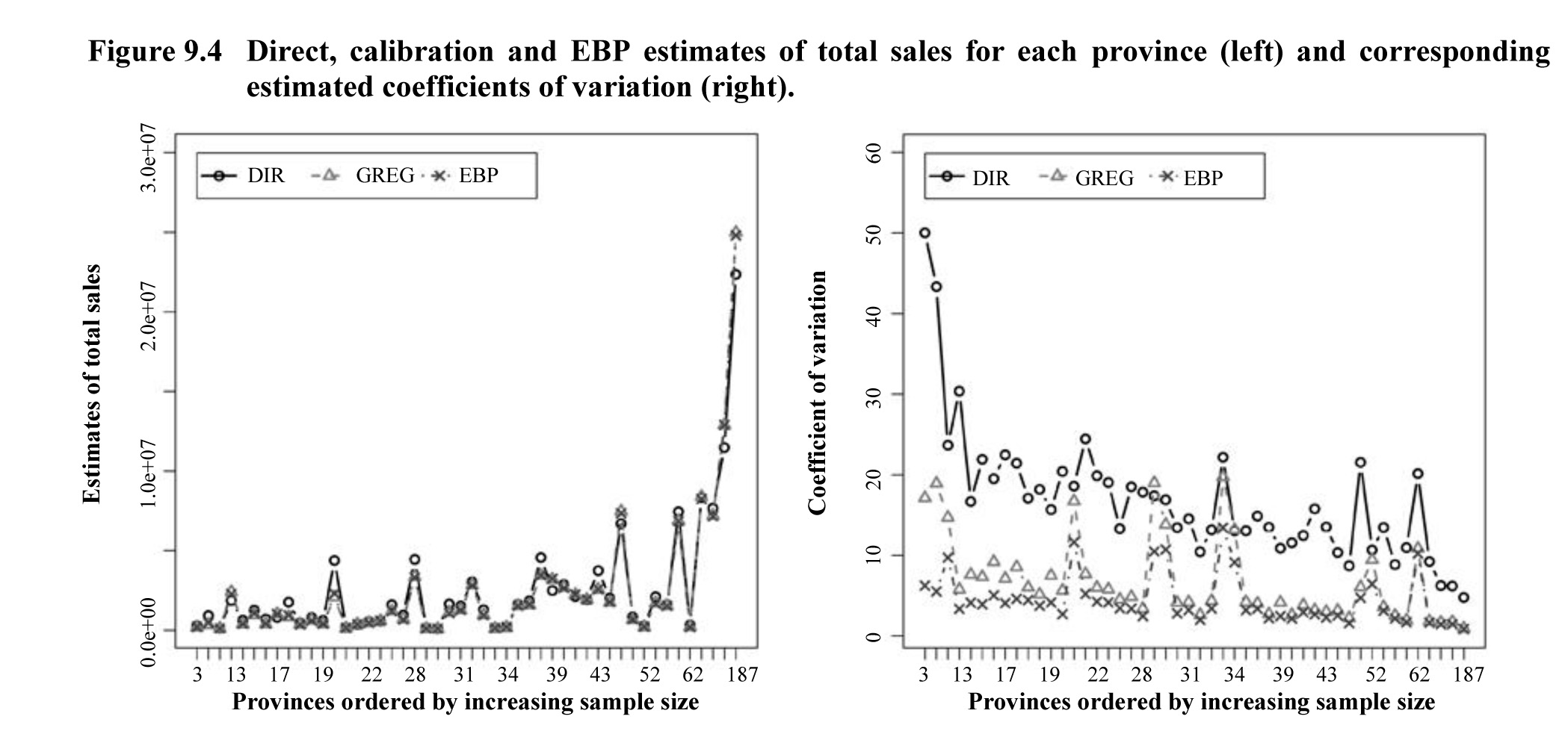
Figure 9.4

Description for Figure 9.4 

Figure made of two graphs. The first one shows the direct, calibration and EBP estimates of total sales for each province. The estimates of total sales are on the y-axis, ranging from 0 to 3.0e+07. Provinces ordered by increasing sample size are on the x-axis, ranging from 3 to 187. The three types of estimates take very similar values for all provinces except for a couple of provinces with the larger sample sizes, where the basic direct estimator takes slightly smaller values. The second graph shows the coefficients of variation of the direct, calibration and EBP estimates of total sales for each province. The coefficient of variation is on the y-axis, ranging from 0 to 60. Provinces ordered by increasing sample size are on the x-axis, ranging from 3 to 187. EBP estimators perform uniformly better than the other estimators in terms of estimated CV, keeping the CV values below 10% for practically all provinces, whereas GREG estimator obtains CV values above 10% for the provinces with the smallest sample sizes. There are some peaks in the estimated CVs for some provinces with not necessarily the smallest sample sizes. These larger CV values are due to the presence of zero purchases and sales of the considered product in many tobacco shops for those particular provinces (that particular product is not acquired every month). Clearly, the direct estimator performs the worst in terms of efficiency.

Table A.1 in the Appendix reports direct, LCAL and EBP estimates of province total sales of the product supplemented with their estimated CVs. This table confirms the better performance of EBP in terms of estimated CV under the nested error model, specially for those provinces with small sample sizes. Finally, the direct estimator performs poorly in terms of CV even if the bias due to cut-off sampling is not accounted for.


Date modified: