Small area estimation methods under cut-off sampling
Section 8. Simulation experiments
8.1 Aims and
general description
In this section, we describe simulation experiments designed
to compare the small sample properties of the estimators of
discussed above in the context of cut-off
sampling. Specifically, we compare the naïve direct estimator
calibration estimators
and
and the EBLUP under the nested error model
under two different scenarios. In the first
scenario, the values of the target variable for all the population units are
generated from the same model; in the second, included and excluded units are
generated from different models.
In the absence of cut-off sampling, calibration estimators
are design-consistent as the domain size
increases even if the corresponding model does
not hold, but this is not the case for model-based estimators. On the other
hand, under the corresponding model, the EBLUP of a linear parameter is
approximately the most efficient linear and unbiased estimator, so making
simulations under a model would not provide any additional knowledge. The
purpose here is to see whether the model-based predictors also perform well
with respect to the (cut-off sampling) design. For this reason, we run design-based
simulations by generating one population vector
from the nested error model in (5.1), keeping
it fixed and repeatedly drawing a new cut-off sample in each MC simulation.
Allocation of units to the sets of included or excluded units is done by
generating a random binary variable
for each unit
and area
The units
with
are assigned to
and those with
to
In each Monte Carlo (MC) replicate, samples
are drawn, independently for each domain
from the
units,
8.2 Common
regression model
We consider a population of
20,000 individuals divided into
80 domains with the same size
250,
We consider three auxiliary variables, with
values generated as
The binary variables
determining the allocation of units in
or
for each domain
are generated independently as
where the probabilities
are related to the vector of auxiliary
variables
in the form
We take
Based on this value, the total number of
included units (with
from all the domains represents roughly half
of the population.
The values of
the target variable
are generated from the nested error model
(5.1) using
and taking
and
which leads to a determination coefficient
Then, keeping the population values
fixed, we draw
1,000 Monte Carlo samples
Each of these samples is obtained by drawing
independent domain sub-samples
of size
from the units in
by SRSWOR,
The domain sample sizes are taken as
with each sample size repeated for 20
subsequent domains. With the data from the
sample, we compute the basic direct estimator,
calibration estimators at the domain level (LCAL) and at the population level
(LCALN), and EBLUP. Weights,
and
in the calibration estimators (4.3) and (4.6)
respectively are obtained using the function calib from package sampling (Tillé
and Matei, 2016) of R (R Development Core Team, 2016). EBLUPs are obtained
using R package sae (Molina and Marhuenda, 2015), which by default estimates
the model parameters
and
using restricted maximum likelihood (REML).
Let
be a generic estimator of
and
its value obtained with
sample. We evaluate the performance of
estimators in terms of relative bias (RB) and relative root MSE (RRMSE) under
the design, approximated empirically as
Averages across domains of absolute RB and of RRMSE are
also calculated as
Figure 8.1
displays boxplots of percent RB for the considered estimators of the mean
where each boxplot is for the 20 domains in
each group of sample sizes
We can see the large cut-off sampling bias of
the basic direct estimator, with median RB exceeding 20% for all the domain
sample sizes. This cut-off sampling bias is corrected by all the other
estimators. Nevertheless, the LCALN estimator shows wider boxplots. This
estimator gets large bias for some domains probably because its assisting model
is not accounting for the domain effects. The LCAL estimator is based on a model
that accounts for domain effects and performs well in terms of design bias
uniformly for all the domain sample sizes, although EBLUP also performs rather
well in terms of design bias.
Looking now
at the RRMSE in Figure 8.2, we can see the much smaller RRMSEs of EBLUPs
for all the domain sample sizes. The LCAL estimator gets closer RRMSEs as the
domain sample size grows, but for
it gets huge RRMSEs. We have seen that the
LCALN can be substantially biased for some domains and it also has large RRMSEs
for all the domain sample sizes. Thus, in summary, EBLUP exhibits the lowest
design RRMSE and at the same time keeps the design bias under control.
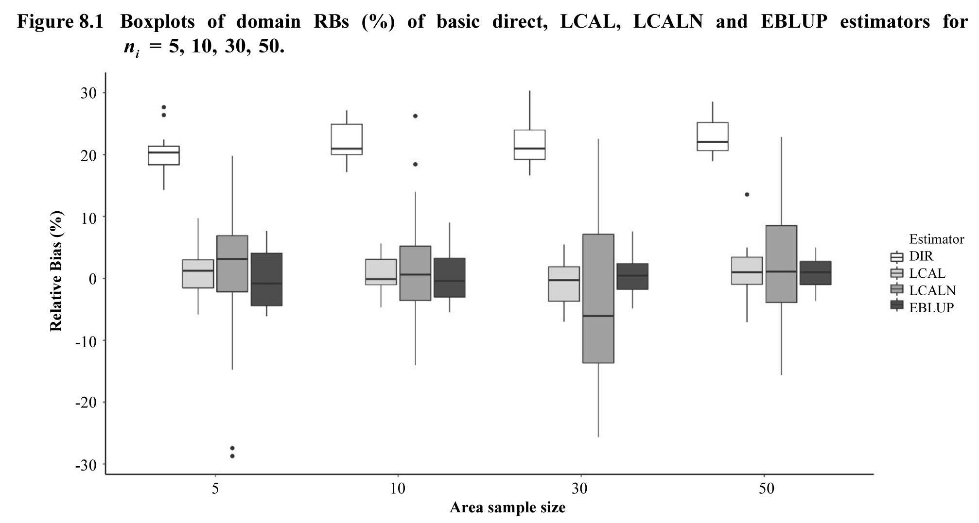
Description for Figure 8.1
Figure
presenting box plots of domain RBs (in %) for four estimators, for four area
sample sizes. The estimators are the basic direct, LCAL, LCALN and EBLUP. The
relative bias in percentages is on the y-axis, ranging from -30 to 30 and the
area sample sizes are on the x-axis, being 5, 10, 30 and 50. The basic direct
estimator cut-off sample bias is large, with median RB exceeding 20% for all
the domain sample sizes. This cut-off sampling bias is corrected by all the
other estimators. Nevertheless, the LCALN estimator shows wider box plots. This
estimator gets large bias for some domains. The LCAL estimator is based on a
model that accounts for domain effects and performs well in terms of design
bias uniformly for all the domain sample sizes, although EBLUP also performs
rather well in terms of design bias.

Description for Figure 8.2
Figure
presenting box plots of domain RRMSEs (in %) for four estimators, for four area
sample sizes. The estimators are the basic direct, LCAL, LCALN and EBLUP. The RRMSE
in percentages is on the y-axis, ranging from 0 to 90 and the area sample sizes
are on the x-axis, being 5, 10, 30 and 50. The RRMSEs of EBLUPs are much
smaller for all the domain sample sizes. The LCAL estimator gets closer RRMSEs
as the domain sample size grows, but for a domain sample size of 5 it gets huge
RRMSEs. The LCALN can be substantially biased for some domains and it also has
large RRMSEs for all the domain sample sizes.
Table 8.1
reports averages across all the domains of absolute RB and RRMSE, together with
% share of squared bias from the total design MSE. We can see again the large
cut-off sampling bias of the basic direct estimator, with a bias share of
100%, in contrast to all other estimators. The LCAL estimator has the smallest
average ARB, followed closely by EBLUP. LCALN performs the best in terms of
bias ratio because of its large MSE. Thus, we consider that LCAL performs
better. As already said, EBLUP clearly performs the best when looking at both
bias and MSE.
Table 8.1
Averages across areas of absolute RB, RRMSE and
for basic direct, LCAL, LCALN and EBLUP (in
percentage)
Table summary
This table displays the results of Averages across areas of absolute RB. The information is grouped by Method (appearing as row headers),
,
and
(appearing as column headers).
| Method |
|
|
|
| DIR |
21.82 |
24.45 |
98.32 |
| LCAL |
2.96 |
27.33 |
2.48 |
| LCALN |
8.97 |
30.44 |
0.04 |
| EBLUP |
3.13 |
4.56 |
0.18 |
8.3 Different regression models
In this
simulation experiment, we preserve the same population values and sampling
scheme as before, but the values of the target variable for the included and
excluded units are generated from models with different parameter values. Of
course, this is not a favorable scenario for the considered model-based
estimators, but it may be realistic since, in practice, the assumed model
cannot be checked for the excluded units. Thus, instead of a constant
for all the population units, we take
for the included units and
for the excluded ones. The values of the
explanatory variables and variance components
and
are taken exactly as before. Again, we draw
1,000 samples
by independent SRSWOR within the units in
domain
with
with the same domain sample sizes
as before. With the sample data from the
sample, we compute basic direct, LCAL, LCALN
and EBLUP estimates of
Figure 8.3
shows boxplots of the corresponding percent RBs for each domain sample size. In
this case, all the estimators are biased, but the bias of the basic direct
estimator becomes huge, exceeding 40% for some of the domains. The bias of LCAL
and EBLUP is kept relatively small for all the domains, but that of LCALN
estimator is still very large in absolute value for some of the domains. In
absence of cut-off sampling, the calibration estimators are asymptotically
design-unbiased as the domain sample size
increases, even if the considered model does
not hold. However, this is not true under cut-off sampling and for this reason
the RBs of calibration estimators do not decrease as
grows. Even under this unfavorable scenario of
different generating models for included and excluded units, EBLUP shows a
moderate bias, which is comparable to that of LCAL estimator, and performs
clearly the best in terms of RRMSE.
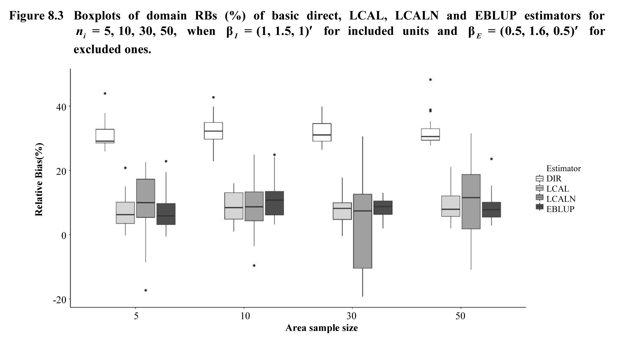
Description for Figure 8.3
Figure
presenting box plots of domain RBs (in %) for four estimators, for four area
sample sizes. For this simulation, the values of the target variable for the
included and excluded units are generated from models with different parameter
values. The estimators are the basic direct, LCAL, LCALN and EBLUP. The
relative bias in percentages is on the y-axis, ranging from -20 to 40 and the
area sample sizes are on the x-axis, being 5, 10, 30 and 50. All the estimators
are biased, but the bias of the basic direct estimator becomes huge, exceeding
40% for some of the domains. The bias of LCAL and EBLUP is kept relatively small
for all the domains, but that of LCALN estimator is still very large in absolute
value for some of the domains. The RBs of calibration estimators do not
decrease as the area sample size grows. The EBLUP estimator shows a moderate
bias, which is comparable to that of LCAL estimator.
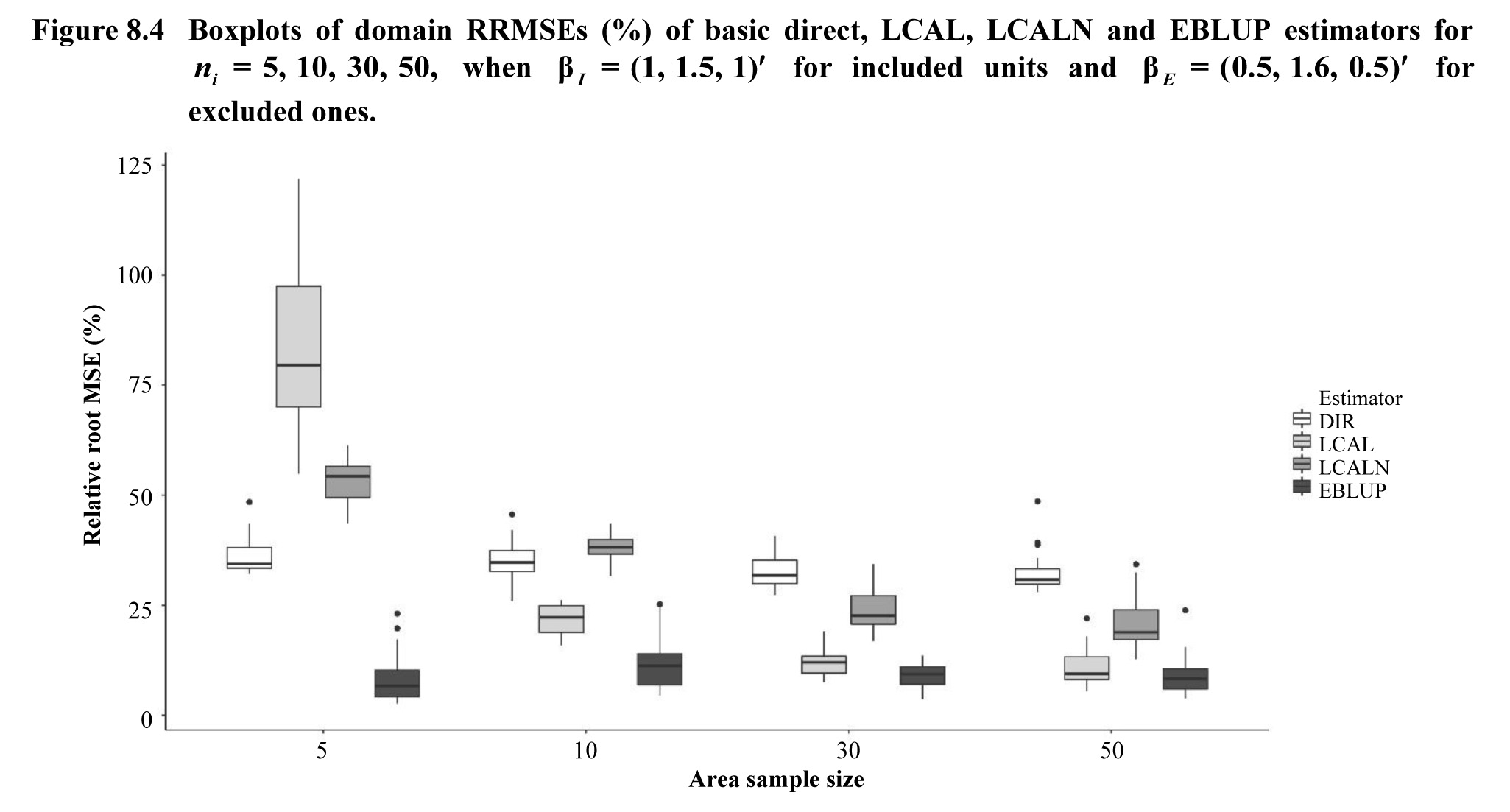
Description for Figure 8.4
Figure
presenting box plots of domain RRMSEs (in %) for four estimators, for four area
sample sizes. For this simulation, the values of the target variable for the
included and excluded units are generated from models with different parameter
values. The estimators are the basic direct, LCAL, LCALN and EBLUP. The RRMSE in
percentages is on the y-axis, ranging from 0 to 125 and the area sample sizes
are on the x-axis, being 5, 10, 30 and 50. The RRMSEs of EBLUPs are smaller for
all the domain sample sizes. The LCAL estimator gets closer RRMSEs as the
domain sample size grows, but for a domain sample size of 5 it gets huge RRMSEs.
The LCALN and basic direct estimators have large RRMSEs for all the domain
sample sizes.
Again, averages across all the domains of absolute RB and
RRMSE are shown in Table 8.2, together with sq. bias ratio. As already
noted, the basic direct estimator has a huge bias, whereas LCAL and EBLUP
estimators keep an
below 10%. LCALN displays the lowest bias
ratio because of a larger MSE. Again, EBLUP shows the best performance in terms
of efficiency, with an average RRMSE also below 10%.
Table 8.2
Averages across areas of absolute RB, RRMSE and
for basic direct, LCAL, LCALN and EBLUP, when
for included units and
for excluded ones (in percentage)
Table summary
This table displays the results of Averages across areas of absolute RB. The information is grouped by Method (appearing as row headers),
,
and
(appearing as column headers).
| Method |
|
|
|
| DIR |
31.78 |
34.11 |
99.87 |
| LCAL |
8.47 |
30.83 |
77.43 |
| LCALN |
12.75 |
34.49 |
29.56 |
| EBLUP |
8.73 |
9.48 |
75.78 |
The simulation experiment was repeated taking a value of
further away from
making the two regression models differ
substantially. Results are not included due to space constraints but, as one
would expect, RB and RRMSE values increase for all estimators, but conclusions
are similar to the last experiment. The basic direct estimator gets the largest
RB, calibration estimators and EBLUP clearly reduce the cut-off sampling bias
of the basic direct estimator and EBLUP gets smaller RRMSE, specially for the
domains with the smallest sample sizes.
