Local polynomial estimation for a small area mean under informative sampling
Section 5. Simulation study
The set-up of the
simulation study follows the one used in Verret et al. (2015). We
considered a population with
15 small areas and
15 units within each small area. The relatively
small number of small areas and units within areas were chosen so as to
alleviate the computational burden. We used a single auxiliary variable
The
population
-values were generated from a gamma
distribution with mean 10 and variance 50. The population
-values were generated by the following model
where
and
with
0.5 and
2.
We considered a single sample size,
3, within a small
area. We used Conditional Poisson Sampling (CPS) to select unequal probability
samples within the small areas, with probabilities proportional to specified
sizes
(see Tillé,
2006, Chapter 5). We considered two different choices of the sizes
in the
simulation study. The first choice uses
where
The size
measures (5.2) are equivalent to those used by Pfeffermann and Sverchkov (2007)
in their simulation study and satisfy the relationship (2.5) on the weights
The second choice of size measures, following
Asparouhov (2006), involves two different types of size measures: invariant (I)
and non-invariant (NI). For the invariant case,
is
independent of
given
otherwise, it is called non-invariant.
Invariant size measures are given by
Non-invariant
size measures are taken as
where the
random pair
is
generated independently of
using
the same distributions as
and
These
size measures were used by Asparouhov (2006). The
coefficient
controls
for the variation of the weights and the value
controls
the level of informativeness of the sampling design. We chose
0.5 and
and
corresponding to several levels of
informativeness generated by
in (5.3)
and (5.4). Increasing
decreases informativeness, with
corresponding to non-informative sampling. If
some of the
exceeded
one, they were set to one, and the probabilities were recomputed for the
remaining units.
5.1 Performance of
the local polynomial estimator of
We compared the
bias and mean squared error of the estimators
and
The
EBLUP estimator
based on
(1.1) assumes that the sample model coincides with the population model,
thereby ignoring the informativeness of the sampling design. We studied two versions of
investigated by Verret et al. (2015) for
various choices of
that
account for informativeness. They are
EBLUP estimators based on the augmented sample model (1.2). They are denoted as
when
and
when
We
report results only for these
functions, as
they outperform others given in Verret et al. (2015). Finally,
represents our new local polynomial estimator.
The bias and the
mean squared error of the estimators were computed using
1,000 simulated samples selected under a design-model approach. For each run,
we first
generated the population
-values under the population model (5.1) and
computed
the mean
of the small area
in the
generated population. Samples of sizes
were
then selected within the small areas using CPS with probabilities proportional
to specified sizes
given by
(5.2) for the Pfeffermann and Sverchkov (2007) (PS) size measures, and (5.3)
and (5.4) corresponding to the invariant and non-invariant cases in the case of
the Asparouhov (2006) (AP) size measures. From each simulated sample
the
estimates
and
were
computed for each small area
An
optimal bandwidth
was
found for
using
the cross-validation criterion. A grid of the form (0.01, 0.02, 0.03,…,
0.15) covered the possible values for
in
populations generated by (5.1).
For a given
estimator of the small area mean
we considered
the following performance measures:
Average Absolute Bias
where
Average Root Mean Squared Error
Table 5.1
reports on the average absolute bias
of
estimators
and
under
the PS size measures (5.2) and AP size measures (5.3 and 5.4) for
and
Table 5.1
Average absolute bias for the PS and AP size measures
Table summary
This table displays the results of Average absolute bias
for the PS and AP size measures. The information is grouped by Estimator
Generation of
(appearing as row headers),
without
and
and (appearing as column headers).
| Estimator |
without
|
|
|
|
| Generation of |
| PS |
0.309 |
0.020 |
0.004 |
0.011 |
| AP |
|
I |
0.431 |
0.002 |
0.036 |
0.004 |
| NI |
0.425 |
0.010 |
0.035 |
0.005 |
|
|
I |
0.206 |
0.017 |
0.022 |
0.024 |
| NI |
0.219 |
0.019 |
0.016 |
0.016 |
|
|
I |
0.139 |
0.005 |
0.012 |
0.033 |
| NI |
0.137 |
0.008 |
0.013 |
0.019 |
|
|
I |
0.008 |
0.008 |
0.008 |
0.026 |
| NI |
0.006 |
0.006 |
0.006 |
0.021 |
As observed in Verret et al. (2015), the
of the
EBLUP estimator
with
just the auxiliary variable
is quite
a bit larger than those based on the augmented models
and
and the
local polynomial method. This holds regardless of how the size measures have
been generated (PS or AP). The
of
attains
its highest value (0.431) when the design is very informative
and
decreases as
increases. This observation also holds for the
estimators based on the augmented models. The inclusion of
or
as an
augmenting variable, in the model results in small
with the
highest being 0.036. Comparing the
of the
local polynomial estimator
to those
associated with the VRH augmented models, we observe that they are comparable
for
and
and
slightly larger for
Table 5.2 reports the simulation results
on the average root mean squared error
of the
estimators for both the PS size measures (5.2) and the AP size measures (5.3
and 5.4) for
and
The
EBLUP,
based on
model (1.1) without the augmenting variable
has the
largest
(0.740
for I and 0.752 for NI) for the AP size measures corresponding to
and
0.685 for the PS size measure. The
decreases as
increases: 0.608 for I and 0.610 for NI in the
case of non-informative sampling
The
for
and
are
significantly smaller than those associated with
when
sampling is very informative
and for the PS size measure. There are small
differences in terms of
between
our non-parametric approach and the parametric approach in Verret et al.
(2015).
Table 5.2
Average root mean squared error
for the PS and AP size measures
Table summary
This table displays the results of Average root mean squared error
for the PS and AP size measures. The information is grouped by Estimator
Generation of
(appearing as row headers),
without ,
, ,
and
(appearing as column headers).
| Estimator |
without
|
|
|
|
| Generation of
|
| PS |
0.685 |
0.229 |
0.200 |
0.200 |
| AP |
|
I |
0.740 |
0.089 |
0.170 |
0.087 |
| NI |
0.752 |
0.158 |
0.200 |
0.149 |
|
|
I |
0.644 |
0.562 |
0.568 |
0.557 |
| NI |
0.650 |
0.557 |
0.555 |
0.555 |
|
|
I |
0.617 |
0.588 |
0.591 |
0.612 |
| NI |
0.619 |
0.587 |
0.589 |
0.607 |
|
|
I |
0.608 |
0.619 |
0.621 |
0.626 |
| NI |
0.610 |
0.622 |
0.625 |
0.629 |
When the sampling is less informative
the
local linear estimator
is
better than
but its
is
slightly larger than those associated with the parametric estimators
and
In this
case, we observe that the estimated function
is close
to a flat line, and this implies that the local linear approximation is not as
appropriate. This explains why
is
slightly worse than
and
when the
level of informativeness of the sampling is low. A local polynomial estimator
performs well when the function
is
meaningfully non-constant.
When the sample is non-informative
is
better than
and
in both
invariant and non-invariant case. This conclusion is somewhat different from
that of Verret et al. (2015) where for
their
estimators
and
have
equal
and
values.
Verret et al. (2015) used both larger populations and samples, and this
may explain why their augmented models produced estimators as good as the
population model under non-informative sampling designs. Under our simulation
set-up, we found that the
and
of the
EBLUP are small for
values
larger than 6: this corresponds to a sample design that is almost
non-informative. In this case, we
recommend using EBLUP.
5.2 Performance of
the MSE estimators
We now turn to the
performance of the bootstrap procedures for estimating the MSEs of the EBLUP,
VRH and local polynomial estimators. Let
be an
estimator of
and
be the
bootstrap estimator of
From
1,000
simulated populations and samples, we
first computed measures of MSE values as
where
is the
true mean, and
is the
value of the estimator for the
population. Let
be the
bootstrap estimator of
It is
denoted as
for the
EBLUP estimator
and
corresponds to the parametric (unconditional) bootstrap method given by
equation (4.2). For our local polynomial estimator
and the
Verret et al. (2015) estimators,
and
the mse
values, denoted as
and
for
and
respectively, are computed using the
conditional parametric bootstrap method of Section 4. For each selected
sample in the
simulated population
we used
400 bootstraps to compute the
value of
that we
denote as
We
considered two measures to evaluate the performance of
average
absolute relative bias and average confidence interval. These measures are
defined as follows:
Average Absolute Relative Bias:
where
Average Confidence Level:
where
and
Table 5.3 reports
simulation results on the average relative bias
of the
MSE estimators for both the PS size measures (5.2) and Asparouhov size measures
(5.3 and 5.4) for
and
Table 5.3
Average relative bias (%) of mse
for the PS and AP size measures
Table summary
This table displays the results of Average relative bias (%) of mse
for the PS and AP size measures. The information is grouped by Estimator
Generation of
(appearing as row headers),
without , , ,
and
(appearing as column headers).
| Estimator |
without
|
|
|
|
| Generation of
|
| PS |
25.4 |
3.9 |
3.4 |
7.7 |
| AP |
|
I |
39.9 |
9.7 |
14.4 |
7.5 |
| NI |
46.6 |
4.1 |
8.7 |
10.0 |
|
|
I |
16.0 |
2.9 |
3.8 |
5.9 |
| NI |
21.4 |
3.8 |
3.5 |
5.8 |
|
|
I |
13.4 |
6.1 |
6.4 |
5.8 |
| NI |
15.4 |
7.3 |
7.4 |
8.8 |
|
|
I |
4.6 |
4.2 |
4.5 |
6.2 |
| NI |
6.1 |
6.4 |
6.3 |
6.9 |
The
of
based on
the model without the augmenting variable
is very
large when the sampling is very informative
39.9%
for I and 46.6% for NI. The
gradually decreases to around 5% under
non-informative sampling
The
of both
the parametric and non-parametric estimators are smaller in general than 10%,
with the exception of 14.4% for the
estimator
that uses
as an
augmenting variable.
Table 5.4 reports
simulation results on the average confidence level
associated with the MSE estimators for both
the PS size measures (5.2) and the AP size measures (5.3 and 5.4) for
and
and
nominal level of 0.95.
Table 5.4
Average confidence level of mse
for the PS and AP size measures
Table summary
This table displays the results of Average confidence level of mse
for the PS and AP size measures. The information is grouped by Estimator
Generation of
(appearing as row headers),
without , , and
(appearing as column headers).
| Estimator |
without
|
|
|
|
| Generation of
|
| PS |
0.898 |
0.937 |
0.941 |
0.936 |
| AP |
|
I |
0.856 |
0.918 |
0.908 |
0.928 |
| NI |
0.834 |
0.930 |
0.920 |
0.934 |
|
|
I |
0.916 |
0.937 |
0.936 |
0.932 |
| NI |
0.907 |
0.936 |
0.933 |
0.936 |
|
|
I |
0.922 |
0.927 |
0.926 |
0.934 |
| NI |
0.918 |
0.930 |
0.933 |
0.926 |
|
|
I |
0.937 |
0.935 |
0.935 |
0.938 |
| NI |
0.934 |
0.934 |
0.933 |
0.931 |
The EBLUP
estimator
has the
worst coverage when the sample design is very informative. The coverage
improves as the design becomes less informative. The coverage of the other
estimators is between 93% and 95%, with the exception of
(the one
that includes
with
coverage slightly lower.
5.3 Inclusion of an augmenting variable
The local polynomial approach results in an automatic way of obtaining a reasonable
augmented model that is a function of the selection probabilities
However,
given that one does not know whether the design is informative or not, should
we always include an augmenting variable in the model? If the sample design is
not informative it is reasonable to use model (1.1). Note that in this case,
including the augmenting variables,
or
has a very small impact either on the absolute
relative bias of the estimator and absolute relative bias of the estimated MSE.
A similar conclusion was obtained in Verret et al. (2015) who used a
larger population and sample size.
The same question arises with respect to the
use of the local polynomial procedure. In this case, the conclusions are not
quite as clear. If the design is very informative, the local polynomial
approach gains in terms of absolute bias and mean squared error when
or
When the
sampling design is less informative
the
parametric approach in Verret et al. (2015) is the better choice, but by a very small margin.
In a practical situation, the value of
is not
known and the decision to use the augmenting variable in a parametric or
nonparametric model should be taken. To this end, we follow the suggested
procedure in Verret et al. (2015) to provide some guidelines on how to
decide on this choice for an arbitrary
data set. Define
and fit
the following model
to the
sample data by ordinary least squares (OLS). The residuals are
where
and
are the
OLS estimators of
and
respectively. Figure 5.1 displays
residual plots of
for the
AP measures
and
in the
invariant case. For
the
relationship between
and
is
clearly linear, suggesting that the design is informative. As
increases,
the design is less informative. Note that
is
constant when
Similar
observations hold for the non-invariant case. For the PS size measures the
graph resembled the one given in Figure 5.1 when
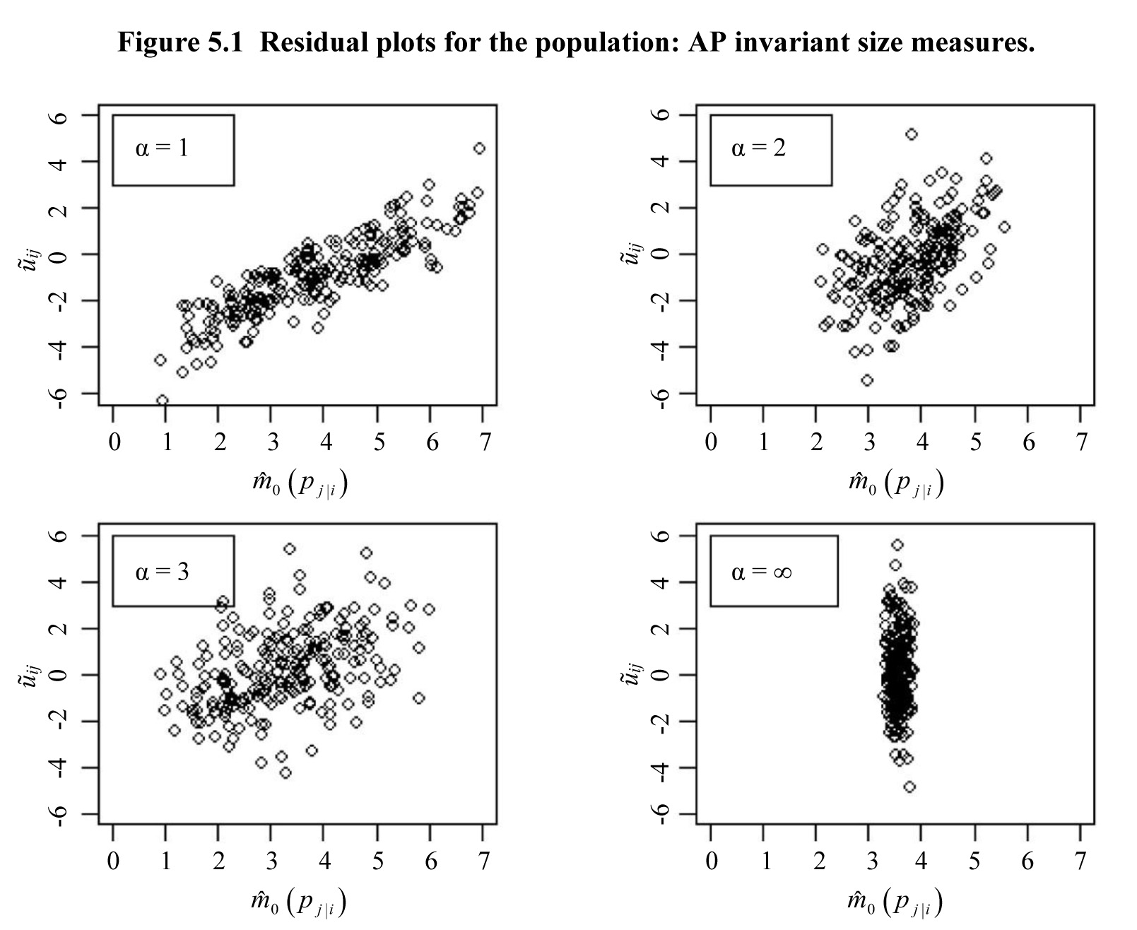
Description for Figure 5.1
Figure presenting four scatter
plots, for
is on the y-axis going from -6 to 6.
is on the x-axis, going from 0 to 7. For
the relationship between
and
is linear. As
increases, the linear relationship fades.
is constant, around 4, when
Table 5.5
provides the estimated correlation
coefficients,
for PS
and AP size measures for
and
Table 5.5
Estimated correlation coefficient
for the PS and AP size measures
Table summary
This table displays the results of Estimated correlation coefficient
for the PS and AP size measures. The information is grouped by Estimated correlation coefficient (appearing as row headers), AP, PS and , , and (appearing as column headers).
| Estimated correlation coefficient |
AP |
PS |
|
|
|
|
|
| I |
NI |
I |
NI |
I |
NI |
I |
NI |
|
|
0.870 |
0.850 |
0.450 |
0.510 |
0.240 |
0.210 |
0.007 |
0.001 |
0.800 |
In terms of
we
noticed in Section 5.1 that
is
better than the estimators based on augmented models for
Results
not presented in Table 5.5 show that for
the absolute value of the correlation
coefficient is less than 0.1. On
the basis of this limited simulation, a user could decide on the choice of the
estimator to use for a real data set as follows: i. If
is larger than 0.5, use
ii. If
is less than 0.1, use
iii.
otherwise use
or
