
A bivariate hierarchical Bayesian model for estimating cropland cash rental rates at the county level
Section 2. Data for modeling non-irrigated cropland cash rental rates
2.1 NASS Cash Rent Survey
NASS implemented a Cash Rent Survey in response to the 2008 Farm Bill. The specific objective of the Cash Rent Survey is to obtain county level estimates of average cash rental rates in three land use categories: non-irrigated cropland, irrigated cropland, and permanent pasture. The data for our study are from the 2009 and 2010 Cash Rent Surveys.
2.1.1 NASS Cash Rent Survey sample design
The 2009 and 2010 Cash Rent Surveys used a stratified sample design. To define the stratification, nine groups were formed on the basis of the dollars rented that an operation reported on previous surveys and censuses. The strata are the intersections of the nine groups and agricultural statistics districts. An agricultural statistics district is a group of contiguous counties within a state that are thought to have similar agricultural characteristics. The sampling fractions within strata are defined so that operations with higher dollars rented on previous surveys and censuses have greater probabilities of selection. The same sample was used for the 2009 and 2010 Cash Rent Surveys, which had a national sample size of approximately 224,000 operations. A unit may respond in only one year either because of nonresponse or because the operation only participated in a rental agreement in one of the two years.
2.1.2 Relationships between 2009 and 2010 non-irrigated cropland cash rents
A direct survey estimator for a particular land use category is a ratio of a weighted sum of the dollars rented to a weighted sum of acres rented. The weight associated with a respondent is the population size of the stratum containing the respondent divided by the number of responding units in that stratum. Berg et al. (2014) explore relationships between direct estimates for two years. For the states considered in Berg et al. (2014), the correlations between the direct estimates for the two years range from 0.20 to 0.99, where the correlation is across counties for a particular state. Because our emphasis is on unit level models, we focus on relationships over time at the unit level.
To measure the correlation between the reported 2009 and 2010 cash rental rates at the unit (farm operator) level, we compute differences between unit-level cash rental rates for non-irrigated cropland and the sample mean for a county. Only individuals that report a cash rental rate for non-irrigated cropland in both years are used to compute the differences. The difference for year is where is the cash rent per acre for non-irrigated cropland reported by operator in county and year and is the sample average of the in county that reported a non-irrigated cropland cash rental rate in both 2009 and 2010. The deviations between individual cash rental rates and the county means for Kansas are plotted in Figure 2.1. The deviations for 2009 and 2010 for Kansas are linearly related, and the correlation between the deviations for 2009 and the deviations for 2010 is 0.7. The extreme values in Figure 2.1 reflect the high variability among the non-irrigated cropland cash rental rates within a county in Kansas.
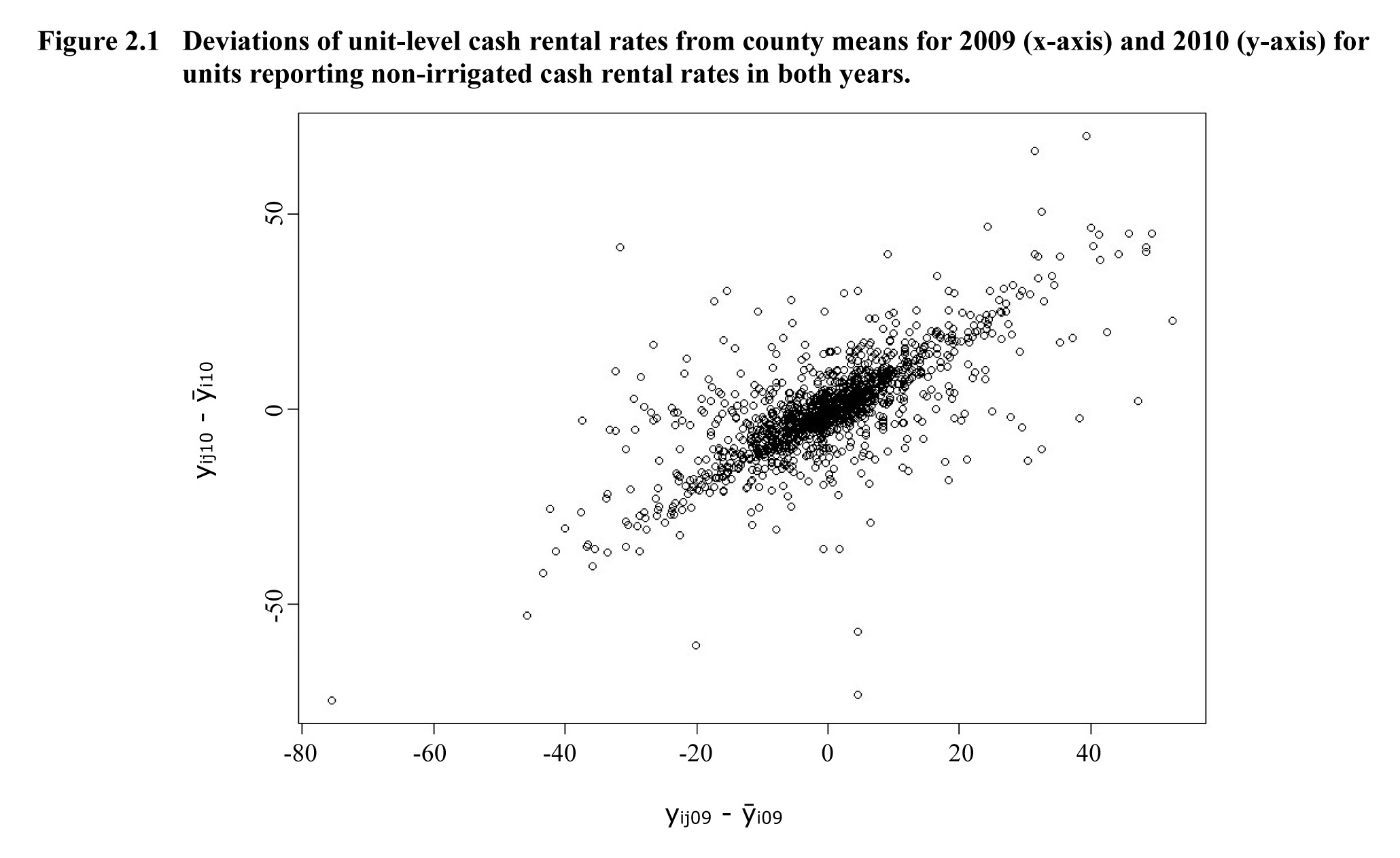
Description for Figure 2.1
Scatter plot graph showing deviations of unit-level cash rental rates from county means for 2009 (x-axis) and 2010 (y-axis) for units reporting non-irrigated cash rental rates in both years, for Kansas. The x-axis, ranges from -80 to 40 and the y-axis, ranges from -50 to 50. A linear relationship between the deviations for 2009 and 2010 can be observed. The correlation between the deviations for 2009 and the deviations for 2010 is 0.7. There are extreme values, caused by the high variability among the non-irrigated cropland cash rental rates within a county in Kansas.
2.2 Auxiliary information
In an effort to improve the precision of the estimators of average cash rental rates at the county level, auxiliary variables were desired that would explain both the variability among the county means as well as the variability among units within a county. Auxiliary information for modeling cash rental rates is available from several sources external to the Cash Rent Survey. The potential covariates divide into three broad categories, depending on whether the covariate relates principally to land quality, the commodity value sold, or other farm characteristics. The list below summarizes the three categories of covariates, indicates whether each covariate is recorded at the county level or the unit level, and specifies if the covariate is only available for a particular state. Unit-level covariates are only available for units in the Cash Rent Survey sample, while area level covariates are treated as population means.
- Land quality
- Four National Commodity Crop Productivity Indexes (NCCPIs) are county-level covariates available for all states. Three climate-specific indexes called NCCPI-corn, NCCPI-wheat, and NCCPI-cotton reflect the quality of the soil for growing non-irrigated crops in three different climate conditions (Dobos, Sinclair and Robotham, 2012). The fourth index, Max-NCCPI, is the maximum of the three climate-specific indexes. The indexes are originally constructed at the level of a “mapunit,” an area that has relatively homogeneous soil properties. The county-level covariates are averages of the indexes across all mapunits in a county.
- An average corn yield across years 2005-2009 is available at the county level for Iowa only. All counties in Iowa have a corn yield estimate available for at least one of the years between 2005 and 2009, and years for which a yield estimate is missing for a county are excluded from the average for that county.
- Because Kansas is more agriculturally diverse than Iowa, no single crop yield is published in at least one year between 2005 and 2009 for all counties of interest. To obtain a covariate that is measured for all counties, we constructed a non-irrigated yield index for Kansas. We first averaged NASS published yields for corn, wheat, and sorghum using the method described for the Iowa corn yields. The average yields were then standardized to have mean zero and variance one. The non-irrigated yield index for a county is defined as the largest of the three standardized yields. (For Texas, availability of crop yield information was too sparse to use to define a covariate).
- Value of the commodity sold
- Total value of production for a county based on the 2007 Census of Agriculture is available for all states.
- Expected sales for an operation (unit) recorded on the NASS list frame are available for all states at the unit-level.
- Other farm
characteristics
- Farm type is a unit level categorical covariate, available for all states. Farms are partitioned into 17 farm types on the NASS list frame. To define a covariate, the farm types are aggregated into two groups: (1) grains/oilseeds, and (2) other.
- Acres rented for non-irrigated cropland recorded on the NASS Cash Rent Survey are available at the unit level for all states.
- Date modified: