Maximum entropy classification for record linkage
Section 6. Simulation study
6.1 Set-up
To explore the practical
feasibility of the unsupervised MEC algorithm for record linkage, we conduct a
simulation study based on the data sets listed in Table 6.1, which are
disseminated by ESSnet-DI (McLeod,
Heasman and Forbes, 2011) and freely
available online. Each record in a data set has associated synthetic key
variables, which may be distorted by missing values and typos when they are
created, in ways that imitate real-life errors (McLeod et al., 2011).
Table 6.1
Data set description (size in parentheses)
Table summary
This table displays the results of Data set description (size in parentheses). The information is grouped by Data set (appearing as row headers), Description (appearing as column headers).
| Data set |
Description |
| Census (25,343) |
A fictional data set to represent some observations from a decennial Census. |
| CIS (24,613) |
Fictional observations from Customer Information System, combined administrative data from the tax and benefit systems. |
| PRD (24,750) |
Fictional observations from Patient Register Data of the National Health Service. |
We consider the linkage
keys forename, surname, sex, and date of birth (DOB). To model the key variables,
we divide DOB into 3 key variables (Day, Month, Year). For text variables such
as forename and surname, we divide them into 4 key variables by using the
Soundex coding algorithm (Copas
and Hilton, 1990, page 290), which
reduces a name to a code consisting of the leading letter followed by three
digits, e.g. Copas C120, Hilton H435. The
twelve key variables for record linkage are presented in Table 6.2.
Table 6.2
Twelve key variables available in the three data sets
Table summary
This table displays the results of Twelve key variables available in the three data sets. The information is grouped by Variable (appearing as row headers), Description and No. of Categories (appearing as column headers).
| Variable |
Description |
No. of Categories |
| PERNAME1 |
1 |
First letter of forename |
26 |
| 2 |
First digit of Soundex code of forename |
7 |
| 3 |
Second digit of Soundex code of forename |
7 |
| 4 |
Third digit of Soundex code of forename |
7 |
| PERNAME2 |
1 |
First letter of surname |
26 |
| 2 |
First digit of Soundex code of surname |
7 |
| 3 |
Second digit of Soundex code of surname |
7 |
| 4 |
Third digit of Soundex code of surname |
7 |
| SEX |
Male/Female |
2 |
| DOB |
DAY |
Day of birth |
31 |
| MON |
Month of birth |
12 |
| YEAR |
Year of birth (1910
2012) |
103 |
We set up two scenarios
to generate linkage files. We use the unique identification variable
(PERSON-ID) for sampling, which are available in all the three data sets. We
sample and individuals
from PRD and CIS, respectively. Let be the
proportion of records in the smaller file (PRD) that are also selected in the
larger file (CIS), by which we can vary the degree of overlap, i.e. the set of
matched individuals between and We use or 0.3 under
either scenario.
Scenario-I (Non-informative)
- Sample individuals
randomly from Census.
- Sample randomly from
these as the
individuals of PRD, denoted by
- Sample randomly from
these as the
individuals of CIS, denoted by
Under this scenario both and are
non-informative for the key-variable distribution. For any given we have and where is the random
number of matched individuals between the simulated files and
Scenario-II (Informative)
- Sample randomly from
Census PRD CIS,
denoted by from PRD.
- Sample randomly from as the matched
individuals, denoted by
- Sample randomly from having and odd MON, denoted by Let be the sampled
individuals of CIS.
Under this scenario the
key-variable distribution is the same in whether or not but it is
different for the records or Hence,
scenario-II is informative. For any given we have fixed and
6.2 Results: Estimation
For the unsupervised MEC
algorithm given in Section 4.1, one can adopt (4.2) or (5.1) for updating Moreover, one
can use (4.4) for directly, or (5.3)
for updating iteratively. In
particular, choosing (5.1) and (4.4) effectively incorporates the procedure of Winkler (1988) and Jaro (1989) for parameter estimation. Note that the MEC approach
still differs to that of Jaro
(1989), with respect to the formation of
the linked set
Table 6.3 compares
the performance of the unsupervised MEC algorithm, using different formulae for
and where the size
of is equal to the
corresponding estimate In addition, we
include estimated
directly from the matched pairs in as if were available
for supervised learning, together with (4.4) for The true
parameters and error rates are given in addition to their estimates.
Table 6.3
Parameters and averages of their estimates, averages of error rates and their estimates, over 200 simulations. Median of estimate of
given as
Table summary
This table displays the results of Parameters and averages of their estimates Scenario I and Scenario II (appearing as column headers).
| Scenario I |
Scenario II |
| Parameter |
Formulae |
Estimation |
Parameter |
Formulae |
Estimation |
|
|
|
|
|
|
|
|
FLR
| MMR |
|
|
|
|
|
|
|
|
|
FLR |
MMR |
|
|
| 0.0008 |
400 |
|
(4.4) |
0.00080 |
400.0 |
397 |
0.0264 |
0.0266 |
0.0357 |
0.0357 |
0.0008 |
400 |
|
(4.4) |
0.00080 |
398.3 |
400 |
0.0230 |
0.0273 |
0.0326 |
0.0326 |
| (4.2) |
(5.3) |
0.00082 |
407.9 |
405 |
0.0425 |
0.0257 |
0.0509 |
0.0509 |
(4.2) |
(5.3) |
0.00080 |
401.4 |
401 |
0.0305 |
0.0277 |
0.0403 |
0.0403 |
| (4.2) |
(4.4) |
0.00083 |
414.7 |
407 |
0.0549 |
0.0244 |
0.0620 |
0.0620 |
(4.2) |
(4.4) |
0.00081 |
405.2 |
404 |
0.0379 |
0.0262 |
0.0467 |
0.0467 |
| (5.1) |
(4.4) |
0.00081 |
406.0 |
405 |
0.0399 |
0.0269 |
0.0503 |
0.0503 |
(5.1) |
(4.4) |
0.00080 |
401.4 |
401 |
0.0316 |
0.0286 |
0.0438 |
0.0438 |
| 0.0005 |
250 |
|
(4.4) |
0.00050 |
251.6 |
249 |
0.0340 |
0.0301 |
0.0370 |
0.0370 |
0.0005 |
250 |
|
(4.4) |
0.00050 |
249.6 |
250 |
0.0284 |
0.0302 |
0.0334 |
0.0334 |
| (4.2) |
(5.3) |
0.00052 |
258.3 |
255 |
0.0559 |
0.0296 |
0.0533 |
0.0533 |
(4.2) |
(5.3) |
0.00050 |
251.8 |
251 |
0.0383 |
0.0320 |
0.0410 |
0.0410 |
| (4.2) |
(4.4) |
0.00053 |
266.9 |
256.5 |
0.0742 |
0.0277 |
0.0680 |
0.0680 |
(4.2) |
(4.4) |
0.00052 |
257.7 |
253 |
0.0513 |
0.0295 |
0.0516 |
0.0516 |
| (5.1) |
(4.4) |
0.00052 |
261.7 |
259 |
0.0676 |
0.0305 |
0.0636 |
0.0636 |
(5.1) |
(4.4) |
0.00051 |
255.4 |
253.5 |
0.0510 |
0.0336 |
0.0520 |
0.0520 |
| 0.0003 |
150 |
|
(4.4) |
0.00030 |
152.3 |
151 |
0.0439 |
0.0356 |
0.0381 |
0.0381 |
0.0003 |
150 |
|
(4.4) |
0.00030 |
150.5 |
150 |
0.0382 |
0.0355 |
0.0350 |
0.0350 |
| (4.2) |
(5.3) |
0.00033 |
165.9 |
156.5 |
0.0873 |
0.0244 |
0.0620 |
0.0620 |
(4.2) |
(5.3) |
0.00031 |
153.0 |
153 |
0.0559 |
0.0377 |
0.0452 |
0.0452 |
| (4.2) |
(4.4) |
0.00041 |
205.4 |
161 |
0.1632 |
0.0308 |
0.1251 |
0.1251 |
(4.2) |
(4.4) |
0.00032 |
158.5 |
155 |
0.0708 |
0.0342 |
0.0558 |
0.0558 |
| (5.1) |
(4.4) |
0.00054 |
271.4 |
169 |
0.3015 |
0.0785 |
0.1639 |
0.1639 |
(5.1) |
(4.4) |
0.00038 |
189.3 |
156 |
0.1414 |
0.0524 |
0.0903 |
0.0903 |
As expected, the best
results are obtained when the parameter is estimated
directly from the matched pairs in i.e., together with (4.4)
for despite by (4.4) is not
exactly unbiased. Nevertheless, the approximate estimator can be
improved, since the profile-EM estimator given by (5.3) is seen to perform
better across all the set-ups, where both are combined with (4.2) for When it comes
to the two formulae of by (4.2) and (5.1),
and the resulting -estimators and
the error rates FLR and MMR, we notice the followings.
- Scenario-I: When
the size of the matched set is relatively
large at there are only
small differences in terms of the average and median of the two estimators of and the
difference is just a couple of false links in terms of the linkage errors. Figures 6.1
shows that (4.2) results
in a few larger errors of than (5.1) over the 200 simulations, when or As the size of the matched set decreases, the
averages and medians of the estimators of resulting from (4.2) and (5.3) are closer to the true values than
those of the other estimators. Especially when the matched set is relatively
small, where the formula (5.1) results in
considerably worse estimation of in every
respect. While this is partly due to the use of (4.4) instead of (5.3), most of the difference is down to the choice of which can be
seen from intermediary comparisons to the results based on (4.2) and (4.4).
- Scenario-II: The
use of (4.2) and (5.3) for the unsupervised MEC algorithm
performs better than using the other formulae in terms of both estimation of and error rates
across the three sizes of the matched set (Figure 6.2). Relatively greater
improvement is achieved by using (4.2) and (5.3) for the smaller matched sets.
The results suggest that
the unsupervised MEC algorithm tends to be more affected by the size of the
matched set under Scenario-I than Scenario-II. Choosing (4.2) and (5.3),
however, seems to yield the most robust estimation of and error rates
against the small size of the matched set regardless the
informativeness of key-variable errors. The reason must be the fact that the
numerator of is calculated
in (5.1) over all the pairs in instead of the
MEC set which seems
more sensitive when the imbalance between and is aggravated,
while the sizes of and remain fixed.
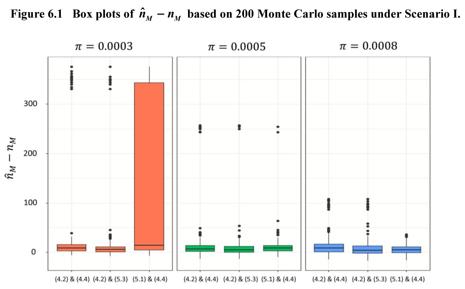
Description of Figure 6.1
Figure presenting box plots of (the error of according to the use of different formulas
((4.2) and (4.4), (4.2) and (5.3), then (5.1) and (4.4)) for the prevalence of
true matches equal
to 0.0003 (orange), 0.0005 (green) and 0.0008 (blue) based on 200 Monte Carlo samples
under Scenario I. In general, the estimate gets worse as reduces. Choosing (4.2) and (5.3) seems to
yield the most robust estimation of
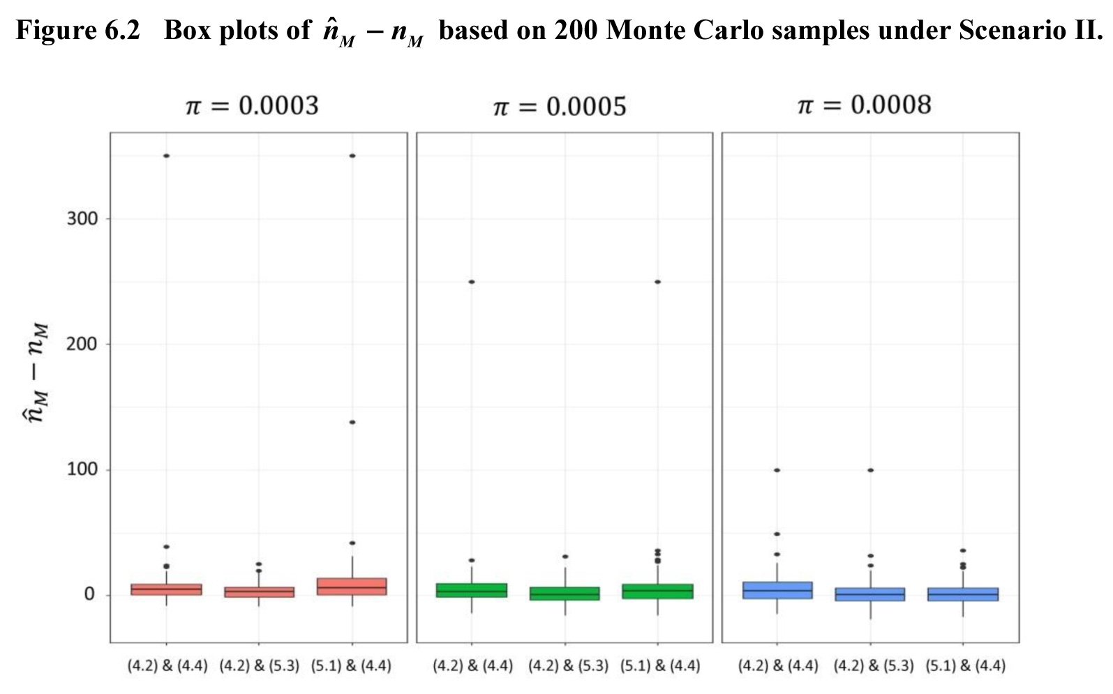
Description of Figure 6.2
Figure presenting box plots of (the error of according to the use of different formulas
((4.2) and (4.4), (4.2) and (5.3), then (5.1) and (4.4)) for the prevalence of
true matches equal
to 0.0003 (orange), 0.0005 (green) and 0.0008 (blue) based on 200 Monte Carlo samples
under Scenario II. In general, the estimate gets worse as reduces. Choosing (4.2) and (5.3) seems to
yield the most robust estimation of The
results suggest that the unsupervised Maximum Entropy Classification algorithm
tends to be more affected by the size of the matched set under Scenario I
than Scenario II.
We also include the
additional results obtained for and 0.1 in the
supplementary material. The estimate (or gets worse as (or reduces, which
is consistent with the previous findings of others, for example, Enamorado,
Fifield and Imai (2019) showed that a greater degree of overlap between data
sets leads to better merging results in terms of the error rates as well as the
accuracy of their estimates. The problem is also highlighted by Sadinle (2017). Record linkage in cases of extremely low prevalence of true matches is a
problem that needs to be studied more carefully on its own.
6.3 Results: MEC set
Aiming the MEC set at the
estimated size is generally not
a reasonable approach to record linkage. Record linkage should be guided
directly by the associated uncertainty, i.e. the error rates FLR and MMR, based
on their estimates (4.5) and (4.6), as described in Section 4.2. Note that
this does require the estimation of in addition to
We have
in Table 6.3, because here. It can be
seen that these follow the true FLR more closely than the MMR, especially when is estimated
using the formulae (4.2) and (5.3). This is hardly surprising. Take e.g. the
maximal MEC set that consists
of the pairs whose key variables agree completely and uniquely. Provided
reasonably rich key variables, as the setting here, one can expect the FLR of to be low, such
that even a naïve estimate
probably does not err much. Meanwhile, the
true MMR has a much wider range from one application to another, because the
difference between and is determined
by the extent of key-variable errors, such that the estimate of MMR depends
more critically on that of The situation
is similar for any MEC set beyond as long as remains very
high for any
Table 6.4 shows the
performance of the MEC set using the bisection procedure described in
Section 4.2, across the same set-ups as in Table 6.3. We use only
(4.2) for and (5.3) for to obtain the
corresponding We let the
target FLR be or 0.03, where
the latter is clearly lower than the true FLR of
that is of the size
(Table 6.3), especially when the
prevalence is relatively low (at
under either scenario. The resulting true
(FLR, MMR) and their estimates are given in Table 6.4.
Table 6.4
Parameters and averages of their estimates, averages of error rates and their estimates, over 200 simulations,
Table summary
This table displays the results of Parameters and averages of their estimates Scenario I and Scenario II (appearing as column headers).
| Scenario I |
Scenario II |
| Parameter |
Target
FLR |
Estimation |
Parameter |
Target
FLR |
Estimation |
|
|
|
|
|
|
FLR |
MMR |
|
|
|
|
|
|
|
FLR |
MMR |
|
|
| 0.0008 |
400 |
0.05 |
407.9 |
0.00080 |
401.9 |
0.0313 |
0.0280 |
0.0393 |
0.0527 |
0.0008 |
400 |
0.05 |
401.4 |
0.00080 |
397.8 |
0.0239 |
0.0294 |
0.0337 |
0.0418 |
| 0.03 |
0.00079 |
395.0 |
0.0196 |
0.0328 |
0.0271 |
0.0568 |
0.03 |
0.00079 |
393.1 |
0.0164 |
0.0334 |
0.0256 |
0.0451 |
| 0.0005 |
250 |
0.05 |
258.3 |
0.00050 |
251.9 |
0.0396 |
0.0326 |
0.0385 |
0.0576 |
0.0005 |
250 |
0.05 |
251.8 |
0.00050 |
248.6 |
0.0305 |
0.0361 |
0.0328 |
0.0447 |
| 0.03 |
0.00049 |
246.7 |
0.0246 |
0.0374 |
0.0264 |
0.0650 |
0.03 |
0.00049 |
245.2 |
0.0226 |
0.0416 |
0.0245 |
0.0497 |
| 0.0003 |
150 |
0.05 |
165.9 |
0.00031 |
153.4 |
0.0533 |
0.0403 |
0.0389 |
0.0783 |
0.0003 |
150 |
0.05 |
153.0 |
0.00030 |
150.1 |
0.0445 |
0.0443 |
0.0333 |
0.0514 |
| 0.03 |
0.00030 |
149.3 |
0.0355 |
0.0483 |
0.0256 |
0.0905 |
0.03 |
0.00029 |
147.4 |
0.0322 |
0.0489 |
0.0238 |
0.0588 |
It can be seen that the
MEC algorithm guided by the FLR yields the MEC set whose size is close to the
true across all the
set-ups. Indeed, under Scenario-I, the mean of is closer to than the mean
(or median) of over all the
simulations, which results directly from parameter estimation, especially when
the match set is relatively small (at and the
performance of is most
sensitive. In other words, the fact that differs to the
estimate is not
necessarily a cause of concern for the MEC algorithm guided by targeting the
FLR.
To estimate the MMR by (4.6),
one can either use as the estimate
of or one can use from parameter
estimation based on (4.2) and (5.3). In the former case, one would obtain
. While this
is not unreasonable in absolute terms since is close to here, as can be
seen from comparing the mean of
with that of the true MMR in Table 6.4,
it has a drawback a priori, in that it decreases as the target FLR
decreases, although one is likely to miss out on more true matches when more
links are excluded from the MEC set Using from parameter
estimation directly makes sense in this respect, since the true must remain the
same, regardless the target FLR. However, the estimator
could then become less reliable given
relatively low prevalence where could be
sensitive in such situations.
In short, the estimation
of FLR tends to be more reliable than that of MMR, especially if the prevalence
is relatively
low in its theoretical range The following
recommendations for unsupervised record linkage seem warranted.
- When forming the
MEC set according to the
uncertainty of linkage, it is more robust to rely on the FLR, estimated by (4.5).
- The estimate of
MMR given by (4.6), derived
from the parameter estimate based on (4.2) and (5.3) provides an additional uncertainty
measure. However, one should be aware that this measure can be sensitive when
the prevalence is relatively
low.
- Between two
target values of the FLR, more attention
can be given to the estimate of additional missing matches in compared to given by
ISSN : 1492-0921
Editorial policy
Survey Methodology publishes articles dealing with various aspects of statistical development relevant to a statistical agency, such as design issues in the context of practical constraints, use of different data sources and collection techniques, total survey error, survey evaluation, research in survey methodology, time series analysis, seasonal adjustment, demographic studies, data integration, estimation and data analysis methods, and general survey systems development. The emphasis is placed on the development and evaluation of specific methodologies as applied to data collection or the data themselves. All papers will be refereed. However, the authors retain full responsibility for the contents of their papers and opinions expressed are not necessarily those of the Editorial Board or of Statistics Canada.
Submission of Manuscripts
Survey Methodology is published twice a year in electronic format. Authors are invited to submit their articles in English or French in electronic form, preferably in Word to the Editor, (statcan.smj-rte.statcan@canada.ca, Statistics Canada, 150 Tunney’s Pasture Driveway, Ottawa, Ontario, Canada, K1A 0T6). For formatting instructions, please see the guidelines provided in the journal and on the web site (www.statcan.gc.ca/SurveyMethodology).
Note of appreciation
Canada owes the success of its statistical system to a long-standing partnership between Statistics Canada, the citizens of Canada, its businesses, governments and other institutions. Accurate and timely statistical information could not be produced without their continued co-operation and goodwill.
Standards of service to the public
Statistics Canada is committed to serving its clients in a prompt, reliable and courteous manner. To this end, the Agency has developed standards of service which its employees observe in serving its clients.
Copyright
Published by authority of the Minister responsible for Statistics Canada.
© His Majesty the King in Right of Canada as represented by the Minister of Industry, 2022
Use of this publication is governed by the Statistics Canada Open Licence Agreement.
Catalogue No. 12-001-X
Frequency: Semi-annual
Ottawa
