Bayesian inference for multinomial data from small areas incorporating uncertainty about order restriction
Section 5. Simulated BMI

Table of contents

To have a better comparison between those models, Chen and Nandram (2021) construct a simulated data transformed from BMI using the idea of Pool-Adjacent-Violators Algorithm (PAVA) to have strong order restrictions as $θ_{1} \leq \dots \leq θ_{m} \geq \dots \geq θ_{K},$ (Mair, Hornik and de Leeuw, 2009). It is a simple iterative algorithm for solving the quadratic problem.

Generally, given a sequence of $n$ data points $y_{1}, \dots, y_{n},$ we start with $y_{1}$ on the left. We move to the right until we encounter the first violation $y_{i} > y_{i + 1} .$ Then we replace this pair by their average, and back-average to the left as needed, to get monotonicity. We continue this process to the right, until finally we reach $y_{n} .$ We can have a reconstructed data set to fit our order restrictions better. Fitting models to the simulated data, we can discover the advantage of hierarchical multinomial-Dirichlet model with order restrictions easily.

Figure 5.1

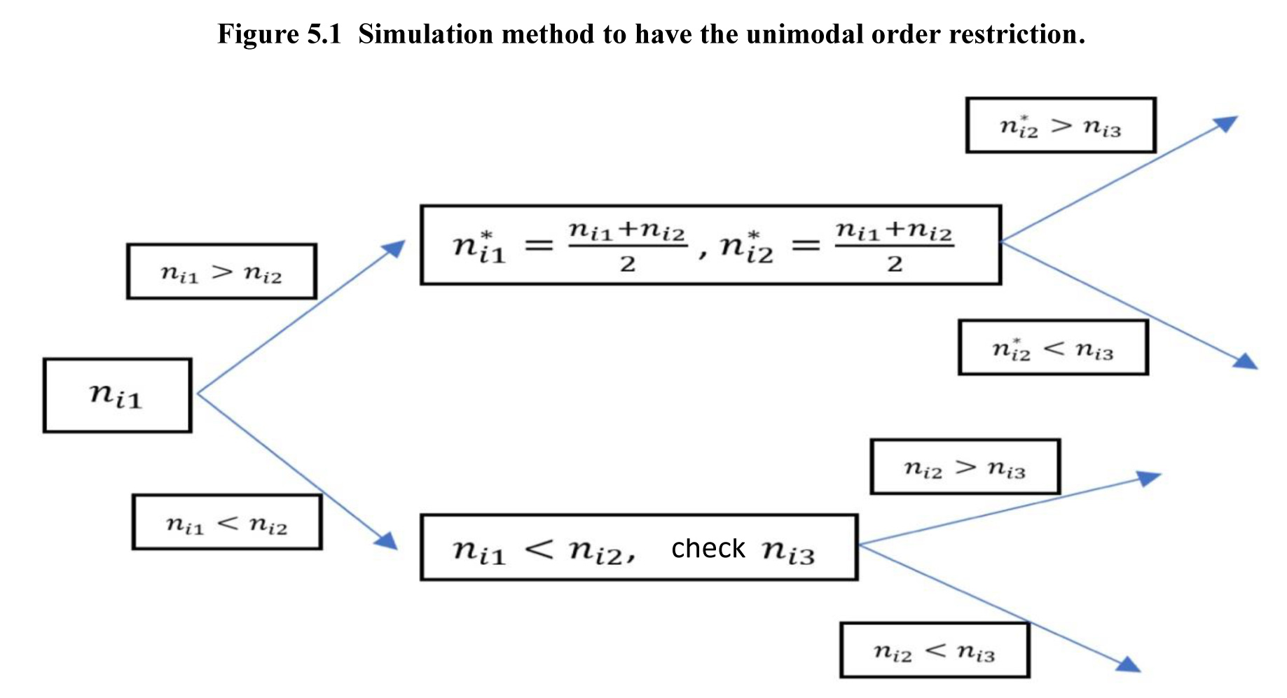
Description of Figure 5.1

Figure presenting the simulation method to have the unimodal order restriction. The method starts with $y_{i}$ on the left. It moves to the right until it encounters the first violation $y_{i} > y_{i + 1} .$ Then it replaces this pair by their average, and back-average to the left as needed, to get monotonicity. It continues this process to the right, until finally it reaches $y_{n} .$

Here, for each county, we start from BMI level 1 to the mode using PAVA to create an increasing sequence. Then from the mode to BMI level 5, we apply PAVA to create a decreasing sequence. To make sure that each BMI level has an integer number, we take the nearest integer that is larger than the mode to replace the mode, and take the nearest integer that is smaller than $n_{i j}$ (except the mode) to replace those non-modes. Now our assembled BMI data have strong order restrictions. But we also notice that our current approach cannot be used for a general case to create an unimodal structure. It works for BMI data when the numbers of level 2 and level 3 are significantly larger than others. Now we have a simulated BMI data which mode is at the third position (overweight).

Table 5.1
LPMLs of model $M_{1},$ $M_{2},$ $M_{3},$ and $M_{4}$ for simulated data, comparison of the four models using LPML
Table summary
This table displays the results of LPMLs of model $M_{1},$ $M_{2},$ $M_{3},$ and $M_{4}$ for simulated data, comparison of the four models using LPML for simulated data. The information is grouped by (équation) (appearing as row headers), (équation) (mode at normal), (équation) (mode at overweight) and (équation) (appearing as column headers).
$M_{1}$	$M_{2}$ (mode at normal)	$M_{3}$ (mode at overweight)	$M_{4}$
-319.83	-330.73	-310.39	-311.26

Since the mode is at the third position, the LPML of $M_{3}$ is significantly larger than others, which is -310.39. The LPML of $M_{4}$ is -311.26, due to the robustness of $M_{4} .$ The LPML of $M_{2}$ is the smallest, which is -330.73. The LPML of $M_{1}$ is -319.83. The LPMLs show that the model with order restrictions can have the best performance if the unimodal assumption is correct. Model $M_{4},$ which incorporates uncertainty about order, has a similar performance as Model $M_{3} .$ In Figure 5.2, $M_{3}$ and $M_{4}$ have consistently large CPO values for 35 counties among those models. $M_{2}$ have lowest CPO values at County 3 and 4, which suggests possible outliers, high-leverage and influential observations. For most of counties, $M_{3}$ has the largest CPOs and $M_{2}$ has the smallest CPOs because of the order restriction assumption may be correct in $M_{3}$ but not in $M_{2} .$

In the simulated BMI data, CPO and LPML are proved to be able to select more adequate models. Model $M_{4}$ is robust and consistent for most cases.

Figure 5.2

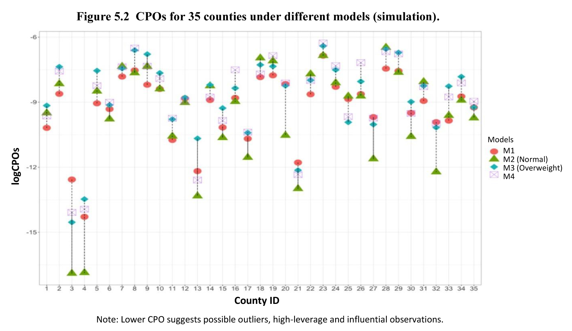
Description of Figure 5.2

Figure presenting the conditional predictive ordinates (CPOs) for the 35 counties under models M1, M2, M3 and M4 with simulated data. Different symbols are used to represent different models’ CPO for all 35 counties. A lower CPO suggests possible outliers, high-leverage and influential observations.

ISSN : 1492-0921

Editorial policy

Survey Methodology publishes articles dealing with various aspects of statistical development relevant to a statistical agency, such as design issues in the context of practical constraints, use of different data sources and collection techniques, total survey error, survey evaluation, research in survey methodology, time series analysis, seasonal adjustment, demographic studies, data integration, estimation and data analysis methods, and general survey systems development. The emphasis is placed on the development and evaluation of specific methodologies as applied to data collection or the data themselves. All papers will be refereed. However, the authors retain full responsibility for the contents of their papers and opinions expressed are not necessarily those of the Editorial Board or of Statistics Canada.

Submission of Manuscripts

Survey Methodology is published twice a year in electronic format. Authors are invited to submit their articles in English or French in electronic form, preferably in Word to the Editor, (statcan.smj-rte.statcan@canada.ca, Statistics Canada, 150 Tunney’s Pasture Driveway, Ottawa, Ontario, Canada, K1A 0T6). For formatting instructions, please see the guidelines provided in the journal and on the web site (www.statcan.gc.ca/SurveyMethodology).

Note of appreciation

Canada owes the success of its statistical system to a long-standing partnership between Statistics Canada, the citizens of Canada, its businesses, governments and other institutions. Accurate and timely statistical information could not be produced without their continued co-operation and goodwill.

Standards of service to the public

Statistics Canada is committed to serving its clients in a prompt, reliable and courteous manner. To this end, the Agency has developed standards of service which its employees observe in serving its clients.

Copyright

Published by authority of the Minister responsible for Statistics Canada.

Use of this publication is governed by the Statistics Canada Open Licence Agreement.

Catalogue No. 12-001-X

Frequency: Semi-annual

Ottawa

Date modified:: 2022-06-21

Language selection

Search and menus

Search

Bayesian inference for multinomial data from small areas incorporating uncertainty about order restriction
Section 5. Simulated BMI

Bayesian inference for multinomial data from small areas incorporating uncertainty about order restriction Section 5. Simulated BMI

Editorial policy

Submission of Manuscripts

Note of appreciation

Standards of service to the public

Copyright

Bayesian inference for multinomial data from small areas incorporating uncertainty about order restriction
Section 5. Simulated BMI