Multiple imputation of missing values in household data with structural zeros
Section 6. Discussion
The
empirical study suggests that the NDPMPM can provide high quality imputations
for categorical data nested within households. To our knowledge, this is the
first parametric imputation engine for nested multivariate categorical data.
The study also illustrates that, with modest sample sizes, agencies should not
expect the NDPMPM to preserve all features of the joint distribution. Of
course, this is the case with any imputation engine. For the NDPMPM, agencies
may be able to improve accuracy for targeted quantities by recoding the data
used to fit the model. For example, one can create a new household-level
variable that equals one when everyone has the same race and equals zero
otherwise, and replace the individual race variable with a new variable that
has levels “1 = race is the same as race of household head”, “2 =
race is white and differs from race of household head”, “3 = race is black
and differs from race of household head”, and so on. The NDPMPM would be
estimated with the household-level same race variable and the new
individual-level race variable. This would encourage the NDPMPM to estimate the
percentages with the same race very accurately, as it would be just another
household-level variable like home ownership. It also would add structural
zeros involving race to the computation. Evaluating the trade offs in accuracy
and computational costs of such recodings is a topic for future research.
The
NDPMPM can be computationally expensive, even with the speed-ups presented in
this article. The expensive parts of the algorithm are the rejection sampling
steps. Fortunately, these can be done easily by parallel processing. For
example, we can require each processor to generate a fraction of the impossible
cases in Section 2.2. We also can spread the rejection steps for the
imputations over many processors. These steps should cut run time by a factor
roughly equal to the number of processors available.
The
empirical study used households up to size four. We have run the model on data
with households up to size seven in reasonable time (a few hours on a standard
laptop). Accuracy results are similar qualitatively. As the household sizes get
large, the model can generate hundreds or even thousands times as many
impossible households as there are feasible ones, slowing the algorithm. In
such cases, the cap-and-weight approach is essential for practical
applications.
Acknowledgements
This
research was supported by grants from the National Science Foundation (NSF SES
1131897) and the Alfred P. Sloan Foundation (G-2-15-20166003).
Appendix
This
is an Appendix to the paper. It contains proof that the rejection sampling step
S9' in Section 3 generates samples from the correct posterior
distribution. It also contains the modified Gibbs sampler for the
cap-and-weight approach and a list of the structural zero rules used in fitting
the NDPMPM model. Finally, we include empirical results for the speedup
approaches mentioned in the paper, using synthetic data, and additional results
for handling missing data using the NDPMPM under a missing completely at random
scenario.
A.1 Proof that the rejection sampling step S9' in
Section 3 generates samples from the correct posterior distribution
The
and
values generated using the rejection sampler
in Step S9' are generated from the full conditionals, resulting in a valid
Gibbs sampler. The proof follows from the properties of rejection sampling (or
simple accept reject). The target distribution is the full conditional for
It can be re-expressed as
where
Our rejection scheme uses
as a proposal for
To show that the draws are indeed from
we need to verify that
where
and that we are accepting each sample with
probability
In our case,
-
and
necessarily.
- By sampling until we obtain a valid sample that
satisfies
we are indeed sampling with probability
A.2 Modified Gibbs sampler for the cap-and-weight
approach
The
modified Gibbs sampler for the cap-and-weight approach replaces steps S1, S3,
S4, S5 and S6 of the Gibbs sampler in the main text as follows.
- S1*. For each
repeat steps S1(a) to S1(e) as before but
modify step S1(f) to: if
return to step (b). Otherwise, set
- S3*. Set
Sample
where
for
- S4*. Set
for
Sample
where
for
and
where
for
and
where
for
and
A.3 List of structural zeros
We
fit the NDPMPM model using structural zeros which involve ages and
relationships of individuals in the same house. The full list of the rules used
is presented in Table A.1. These rules were derived from the 2012 ACS by
identifying combinations involving the relationship variable that do not appear
in the constructed population. This list should not be interpreted as a “true”
list of impossible combinations in census data.
Table A.1
List of structural zeros
Table summary
This table displays the results of List of structural zeros. The information is grouped by Description (appearing as row headers), (appearing as column headers).
| Description |
This is an empty column |
This is an empty column |
Rules common to generating both the synthetic and imputed datasets
|
1 |
Each household must contain exactly one head and he/she must be at least 16 years old. |
| 2 |
Each household cannot contain more than one spouse and he/she must be at least 16 years old. |
| 3 |
Married couples are of opposite sex, and age difference between individuals in the couples cannot exceed 49. |
| 4 |
The youngest parent must be older than the household head by at least 4. |
| 5 |
The youngest parent-in-law must be older than the household head by at least 4. |
| 6 |
The age difference between the household head and siblings cannot exceed 37. |
| 7 |
The household head must be at least 31 years old to be a grandparent and his/her spouse must be at least 17. Also, He/she must be older than the oldest grandchild by at least 26. |
| Rules specific to generating the synthetic datasets |
8 |
The household head must be older than the oldest child by at least 7. |
| Rules specific to generating the imputed datasets |
9 |
The household head must be older than the oldest biological child by at least 7. |
| 10 |
The household head must be older than the oldest adopted child by at least 11. |
| 11 |
The household head must be older than the oldest stepchild by at least 9. |
A.4 Empirical study of the speedup approaches
We
evaluate the performance of the two speedup approaches mentioned in the main
text using synthetic data. We use data from the public use microdata files from
the 2012 ACS, available for download from the United States Census Bureau
(http://www2.census.gov/acs2012_1yr/pums/) to construct a population of 857,018
households of sizes
from which we sample
households comprising
individuals. We work with the variables
described in Table A.2. We evaluate the approaches using probabilities
that depend on within household relationships and the household head.
Table A.2
Description of variables used in the synthetic data illustration
Table summary
This table displays the results of Description of variables used in the synthetic data illustration. The information is grouped by Description of variable (appearing as row headers), Categories (appearing as column headers).
| Description of variable |
Categories |
| Household-level variables |
Ownership of dwelling |
1 = owned or being bought, 2 = rented |
| Household size |
2 = 2 people, 3 = 3 people, 4 = 4 people, |
| 5 = 5 people, 6 = 6 people |
| Individual-level variables |
Gender |
1 = male, 2 = female |
| Race |
1 = white, 2 = black, |
| 3 = American Indian or Alaska native, |
| 4 = Chinese, 5 = Japanese, |
| 6 = other Asian/Pacific islander, 7 = other race, |
| 8 = two major races, |
| 9 = three or more major races |
| Hispanic origin |
1 = not Hispanic, 2 = Mexican, |
| 3 = Puerto Rican, 4 = Cuban, 5 = other |
| Age |
1 = less than one year old, 2 = 1 year old, |
| 3 = 2 years old, ..., 96 = 95 years old |
| Relationship to head of household |
1 = household head, 2 = spouse, 3 = child, |
| 4 = child-in-law, 5 = parent, 6 = parent-in-law, |
| 7 = sibling, 8 = sibling-in-law, 9 = grandchild, |
| 10 = other relative, 11 = partner/friend/visitor, |
| 12 = other non-relative |
We
consider the NDPMPM using two approaches, both moving the values of the
household head to the household level as in Section 4.1 of the main text
and also using the cap-and-weight approach in Section 4.2 of the main
text. The first approach considers
while the second approach considers
and
We compare these approaches to the NDPMPM as
presented in Hu et al., 2018. For each approach, we create
synthetic datasets,
We generate the synthetic datasets so that the
number of households of size
in each
exactly matches
from the observed data. Thus,
comprises partially synthetic data (Little,
1993; Reiter, 2003), even though every released
is a simulated value. We combine the estimates
using using the approach in Reiter (2003). As a brief review, let
be the point estimator of some estimand
and let
be the estimator of variance associated with
For
let
and
be the values of
and
in synthetic dataset
We use
as the point estimate of
and
as the estimated variance of
where
and
We make inference about
using
where
is a
distribution with
degrees of freedom.
For
each approach, we run the MCMC sampler for 20,000 iterations, discarding the
first 10,000 as burn-in and thinning the remaining samples every five
iterations, resulting in 2,000 MCMC post burn-in iterates. We create the
synthetic datasets by randomly sampling from
the 2,000 iterates. We set
and
for each approach based on initial tuning
runs. For convergence, we examined trace plots of
,
and weighted averages of a random sample of
the multinomial probabilities in the NDPMPM likelihood. Across the approaches,
the effective number of occupied household-level clusters usually ranges from
20 to 33 with a maximum of 38, while the effective number of occupied
individual-level clusters across all household-level clusters ranges from 5 to
9 with a maximum of 12.
Based
on MCMC runs on a standard laptop, moving household heads’ data values to the
household level alone results in a speedup of about 63% on the default
rejection sampler while the cap-and-weight approach alone results in a speedup
of about 40%.
Table A.3
shows the 95% confidence intervals for each approach. Essentially, all three
approaches result in similar confidence intervals, suggesting not much loss in
accuracy from the speedups. Most intervals also are reasonably similar to
confidence intervals based on the original data, except for the percentage of
same age couples. The last row is a rigorous test of how well each method can
estimate a probability that can be fairly difficult to estimate accurately. In
this case, the probability that a household head and spouse are the same age
can be difficult to estimate since each individual’s age can take 96 different
values. All three approaches are thus off from the estimate from the original
data in this case. These results suggest that we can significantly speedup the
sampler with minimal loss in accuracy of estimates and confidence intervals of
population estimands.
Table A.3
Confidence intervals for selected probabilities that depend on within-household relationships in the original and synthetic datasets. “Original” is based on the sampled data, “NDPMPM” is the default MCMC sampler described in Section 2.2 of the main text, “NDPMPM w/ HH moved” is the default sampler, moving household heads’ data values to the household level, “NDPMPM capped w/ HH moved” uses the cap-and-weight approach and moving household heads’ data values to the household level. “HH ” means household head and “SP” means spouse
Table summary
This table displays the results of Confidence intervals for selected probabilities that depend on within-household relationships in the original and synthetic datasets. “Original” is based on the sampled data Original, NDPMPM, NDPMPM w/ HH moved and NDPMPM capped w/ HH moved (appearing as column headers).
|
Original |
NDPMPM |
NDPMPM w/ HH moved |
NDPMPM capped w/ HH moved |
| All same race |
|
(0.939, 0.951) |
(0.918, 0.932) |
(0.912, 0.928) |
(0.910, 0.925) |
|
(0.896, 0.920) |
(0.859, 0.888) |
(0.845, 0.875) |
(0.844, 0.874) |
|
(0.885, 0.912) |
(0.826, 0.860) |
(0.813, 0.848) |
(0.817, 0.852) |
|
(0.879, 0.922) |
(0.786, 0.841) |
(0.786, 0.841) |
(0.777, 0.834) |
|
(0.831, 0.910) |
(0.701, 0.803) |
(0.718, 0.819) |
(0.660, 0.768) |
| SP present |
This is an empty cell |
(0.693, 0.711) |
(0.678, 0.697) |
(0.676, 0.695) |
(0.677, 0.695) |
| SP with white HH |
This is an empty cell |
(0.589, 0.608) |
(0.577, 0.597) |
(0.576, 0.595) |
(0.575, 0.595) |
| SP with black HH |
This is an empty cell |
(0.036, 0.043) |
(0.035, 0.043) |
(0.034, 0.042) |
(0.034, 0.042) |
| White couple |
This is an empty cell |
(0.570, 0.589) |
(0.560, 0.580) |
(0.553, 0.573) |
(0.552, 0.572) |
| White couple, own |
This is an empty cell |
(0.495, 0.514) |
(0.468, 0.488) |
(0.461, 0.481) |
(0.463, 0.483) |
| Same race couple |
This is an empty cell |
(0.655, 0.673) |
(0.636, 0.655) |
(0.626, 0.645) |
(0.625, 0.644) |
| White-nonwhite couple |
This is an empty cell |
(0.028, 0.035) |
(0.028, 0.035) |
(0.034, 0.041) |
(0.036, 0.044) |
| Nonwhite couple, own |
This is an empty cell |
(0.057, 0.067) |
(0.047, 0.056) |
(0.045, 0.053) |
(0.045, 0.054) |
| Only mother present |
This is an empty cell |
(0.017, 0.022) |
(0.014, 0.019) |
(0.014, 0.019) |
(0.013, 0.018) |
| Only one parent present |
This is an empty cell |
(0.021, 0.026) |
(0.026, 0.032) |
(0.026, 0.033) |
(0.027, 0.033) |
| Children present |
This is an empty cell |
(0.507, 0.527) |
(0.493, 0.512) |
(0.517, 0.537) |
(0.511, 0.531) |
| Siblings present |
This is an empty cell |
(0.022, 0.028) |
(0.027, 0.034) |
(0.027, 0.033) |
(0.027, 0.033) |
| Grandchild present |
This is an empty cell |
(0.041, 0.049) |
(0.051, 0.060) |
(0.049, 0.058) |
(0.050, 0.059) |
| Three generations present |
This is an empty cell |
(0.036, 0.044) |
(0.037, 0.045) |
(0.042, 0.050) |
(0.040, 0.048) |
| White HH, older than SP |
This is an empty cell |
(0.309, 0.327) |
(0.283, 0.301) |
(0.294, 0.313) |
(0.302, 0.321) |
| Nonhisp HH |
This is an empty cell |
(0.882, 0.894) |
(0.875, 0.888) |
(0.879, 0.891) |
(0.876, 0.889) |
| White, Hisp HH |
This is an empty cell |
(0.071, 0.082) |
(0.074, 0.085) |
(0.072, 0.082) |
(0.073, 0.084) |
| Same age couple |
This is an empty cell |
(0.087, 0.098) |
(0.027, 0.034) |
(0.023, 0.029) |
(0.024, 0.031) |
A.5 Empirical study of missing data imputation
under MCAR
We also evaluate the
performance of the NDPMPM as an imputation method under a missing completely at
random (MCAR) scenario. We use the same data as in Section 5 of the main
text. As a reminder, the data contains
households of sizes
comprising
individuals. We introduce missing values using
a MCAR scenario. We randomly select 80% households to be complete cases for all
variables. For the remaining 20%, we let the variable “household size” be fully
observed and randomly
and independently
blank 50% of each variable for the remaining
household-level and individual-level variables. We use these low rates to mimic
the actual rates of item nonresponse in census data.
Similar to the main text, we
estimate the NDPMPM using two approaches, both combining the rejection step in
Section 4.1 of the main text with the cap-and-weight approach in Section 4.2
of the main text. The first approach considers
while the second approach considers
and
For each approach, we run the MCMC sampler for
10,000 iterations, discarding the first 5,000 as burn-in and thinning the
remaining samples every five iterations, resulting in 1,000 MCMC post burn-in
iterates. We set
and
for each approach based on initial tuning
runs. We monitor convergence as in the main text. For both methods, we generate
completed datasets,
using the posterior predictive distribution of
the NDPMPM, from which we estimate the same probabilities as in the main text.
Figures A.1 and A.2
display each estimated marginal, bivariate and trivariate probability
plotted against its corresponding estimate
from the original data, without missing values. Figure A.1 shows the
results for the NDPMPM with the rejection sampler, and Figure A.2 shows
the results for the NDPMPM using the cap-and-weight approach. For both approaches,
the NDPMPM does a good job of capturing important features of the joint
distribution of the variables as the point estimates are very close to those
from the data before introducing missing values. In short, the results are very
similar to those in the main text, though more accurate.
Table A.4 displays 95%
confidence intervals for selected probabilities involving within-household
relationships, as well as the value in the full population of 764,580
households. The intervals include the two based on the NDPMPM imputation
engines and the interval from the data before introducing missingness. The
intervals are generally more accurate than those presented in the main text.
This is expected since we use lower rates of missingness in the MCAR scenario.
For the most part, the intervals from the NDPMPM with the two approaches tend
to include the true population quantity. Again, the NDPMPM imputation engine
results in downward bias for the percentages of households where everyone is
the same race. As mentioned in the main text, this is a challenging estimand to
estimate accurately via imputation, particularly for larger households.
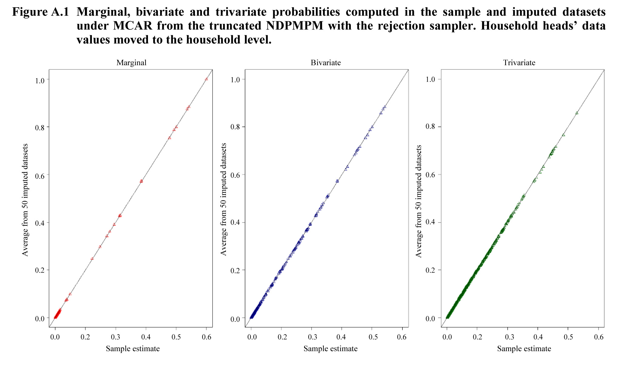
Description for Figure A.1
Figure presenting the marginal, bivariate and trivariate probabilities computed in the sample and imputed datasets under MCAR from the truncated NDPMPM with the rejection sampler (household heads’ data values moved to the household level). There are three scatter plots with a 45° straight line. The three graphs illustrate the marginal, bivariate and trivariate probabilities respectively. The average from 50 imputed datasets is on the y-axis, ranging from 0.0 to 1.0. The sample estimate is on the x-axis, ranging from 0.0 to 0.6. For all three graphs, estimations from imputed data are close to those from the sample, almost on the line.
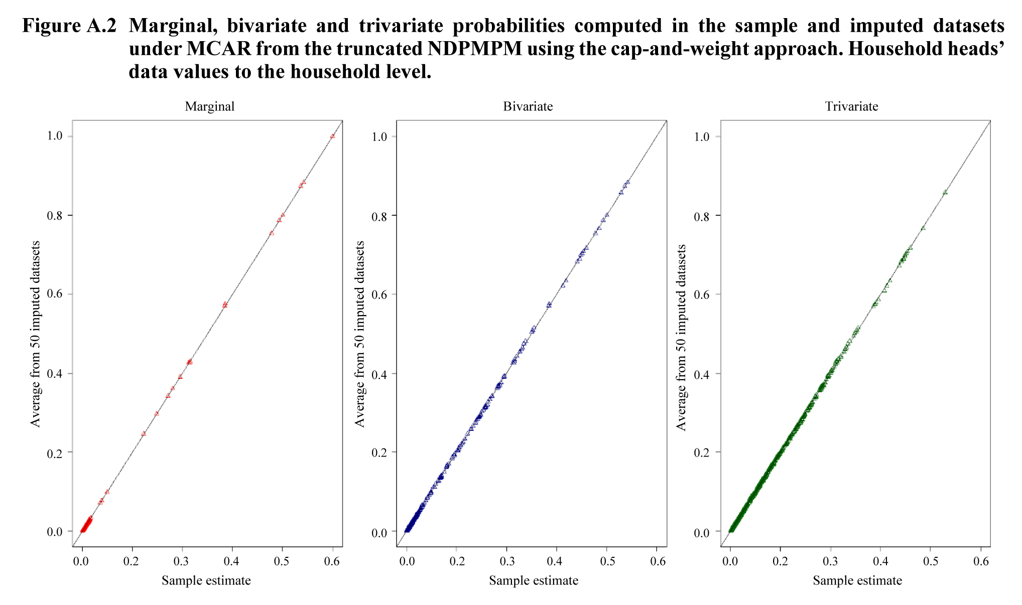
Description for Figure A.2
Figure presenting the marginal, bivariate and trivariate probabilities computed in the sample and imputed datasets under MCAR from the truncated NDPMPM using the cap-and-weight approach (household heads’ data values moved to the household level). There are three scatter plots with a 45° straight line. The three graphs illustrate the marginal, bivariate and trivariate probabilities respectively. The average from 50 imputed datasets is on the y-axis, ranging from 0.0 to 1.0. The sample estimate is on the x-axis, ranging from 0.0 to 0.6. For all three graphs, estimations from imputed data are close to those from the sample, almost on the line.
Table A.4
Confidence intervals for selected probabilities that depend on within-household relationships in the original and imputed datasets under MCAR. “No missing” is based on the sampled data before introducing missing values, “NDPMPM” uses the truncated NDPMPM, moving household heads’ data values to the household level, and “NDPMPM Capped” uses the truncated NDPMPM with the cap-and-weight approach and moving household heads’ data values to the household level. “HH ” means household head, “SP” means spouse, “CH” means child, and “CP” means couple. Q is the value in the full population of 764,580 households
Table summary
This table displays the results of Confidence intervals for selected probabilities that depend on within-household relationships in the original and imputed datasets under MCAR. “No missing” is based on the sampled data before introducing missing values Q, No Missing, NDPMPM and NDPMPM Capped (appearing as column headers).
|
Q |
No Missing |
NDPMPM |
NDPMPM Capped |
| All same race household: |
|
0.942 |
(0.932, 0.949) |
(0.924, 0.944) |
(0.925, 0.946) |
|
0.908 |
(0.907, 0.937) |
(0.887, 0.924) |
(0.890, 0.925) |
|
0.901 |
(0.879, 0.917) |
(0.854, 0.900) |
(0.855, 0.900) |
| SP present |
This is an empty cell |
0.696 |
(0.682, 0.707) |
(0.683, 0.709) |
(0.683, 0.709) |
| Same race CP |
This is an empty cell |
0.656 |
(0.641, 0.668) |
(0.637, 0.664) |
(0.638, 0.665) |
| SP present, HH is White |
This is an empty cell |
0.600 |
(0.589, 0.616) |
(0.590, 0.618) |
(0.590, 0.618) |
| White CP |
This is an empty cell |
0.580 |
(0.569, 0.596) |
(0.568, 0.596) |
(0.568, 0.597) |
| CP with age difference less than five |
This is an empty cell |
0.488 |
(0.465, 0.492) |
(0.422, 0.451) |
(0.422, 0.450) |
| Male HH, home owner |
This is an empty cell |
0.476 |
(0.456, 0.484) |
(0.455, 0.483) |
(0.456, 0.485) |
| HH over 35, no CH present |
This is an empty cell |
0.462 |
(0.441, 0.468) |
(0.438, 0.466) |
(0.438, 0.466) |
| At least one biological CH present |
This is an empty cell |
0.437 |
(0.431, 0.458) |
(0.432, 0.460) |
(0.432, 0.460) |
| HH older than SP, White HH |
This is an empty cell |
0.322 |
(0.309, 0.335) |
(0.308, 0.335) |
(0.306, 0.333) |
| Adult female w/ at least one CH under 5 |
This is an empty cell |
0.078 |
(0.070, 0.085) |
(0.068, 0.084) |
(0.067, 0.083) |
| White HH with Hisp origin |
This is an empty cell |
0.066 |
(0.064, 0.078) |
(0.064, 0.079) |
(0.064, 0.079) |
| Non-White CP, home owner |
This is an empty cell |
0.058 |
(0.050, 0.063) |
(0.048, 0.061) |
(0.048, 0.061) |
| Two generations present, Black HH |
This is an empty cell |
0.057 |
(0.053, 0.066) |
(0.053, 0.066) |
(0.053, 0.067) |
| Black HH, home owner |
This is an empty cell |
0.052 |
(0.046, 0.058) |
(0.046, 0.059) |
(0.046, 0.059) |
| SP present, HH is Black |
This is an empty cell |
0.039 |
(0.032, 0.042) |
(0.032, 0.043) |
(0.032, 0.042) |
| White-nonwhite CP |
This is an empty cell |
0.034 |
(0.029, 0.039) |
(0.032, 0.044) |
(0.032, 0.044) |
| Hisp HH over 50, home owner |
This is an empty cell |
0.029 |
(0.025, 0.034) |
(0.025, 0.035) |
(0.025, 0.035) |
| One grandchild present |
This is an empty cell |
0.028 |
(0.023, 0.033) |
(0.024, 0.034) |
(0.024, 0.034) |
| Adult Black female w/ at least one CH under 18 |
This is an empty cell |
0.027 |
(0.028, 0.038) |
(0.027, 0.037) |
(0.027, 0.037) |
| At least two generations present, Hisp CP |
This is an empty cell |
0.027 |
(0.022, 0.031) |
(0.022, 0.031) |
(0.022, 0.031) |
| Hisp CP with at least one biological CH |
This is an empty cell |
0.025 |
(0.020, 0.028) |
(0.019, 0.028) |
(0.019, 0.028) |
| At least three generations present |
This is an empty cell |
0.023 |
(0.020, 0.028) |
(0.019, 0.028) |
(0.019, 0.028) |
| Only one parent |
This is an empty cell |
0.020 |
(0.016, 0.024) |
(0.016, 0.024) |
(0.016, 0.024) |
| At least one stepchild |
This is an empty cell |
0.019 |
(0.018, 0.026) |
(0.018, 0.027) |
(0.018, 0.027) |
| Adult Hisp male w/ at least one CH under 10 |
This is an empty cell |
0.018 |
(0.017, 0.025) |
(0.016, 0.025) |
(0.016, 0.025) |
| At least one adopted CH, White CP |
This is an empty cell |
0.008 |
(0.005, 0.010) |
(0.005, 0.010) |
(0.005, 0.010) |
| Black CP with at least two biological children |
This is an empty cell |
0.006 |
(0.003, 0.007) |
(0.003, 0.007) |
(0.003, 0.007) |
| Black HH under 40, home owner |
This is an empty cell |
0.005 |
(0.005, 0.009) |
(0.005, 0.010) |
(0.005, 0.011) |
| Three generations present, White CP |
This is an empty cell |
0.005 |
(0.004, 0.008) |
(0.004, 0.010) |
(0.004, 0.009) |
| White HH under 25, home owner |
This is an empty cell |
0.003 |
(0.002, 0.005) |
(0.004, 0.009) |
(0.004, 0.009) |
References
Andridge, R.R., and Little, R.J.A. (2010). A review of
hot deck imputation for survey non-response. International Statistical Review, 78(1), 40-64.
Bennink, M., Croon, M.A., Kroon, B. and Vermunt, J.K. (2016).
Micro-macro multilevel latent class models with multiple discrete
individual-level variables. Advances in
Data Analysis and Classification.
Chambers, R., and Skinner, C. (2003). Analysis of Survey
Data, Wiley Series in Survey Methodology, Wiley.
Dunson, D.B., and Xing, C. (2009). Nonparametric Bayes
modeling of multivariate categorical data. Journal
of the American Statistical Association, 104, 1042-1051.
Hu, J., Reiter, J.P. and Wang, Q. (2018). Dirichlet
process mixture models for modeling and generating synthetic versions of nested
categorical data. Bayesian Analysis,
13, 183-200.
Ishwaran, H., and James, L.F. (2001). Gibbs sampling
methods for stick-breaking priors. Journal
of the American Statistical Association, 161-173.
Kalton, G., and Kasprzyk, D. (1986). The treatment of
missing survey data. Survey Methodology,
12, 1, 1-16. Paper available at https://www150.statcan.gc.ca/n1/en/pub/12-001-x/1986001/article/14404-eng.pdf.
Little, R.J.A. (1993). Statistical analysis of masked
data. Journal of Official Statistics,
9, 407-426.
Manrique-Vallier, D., and Reiter, J.P. (2014). Bayesian
estimation of discrete multivariate latent structure models with structural
zeros. Journal of Computational and
Graphical Statistics, 23, 1061-1079.
Murray, J.S., and Reiter, J.P. (2016). Multiple
imputation of missing categorical and continuous values via Bayesian mixture
models with local dependence (forthcoming). Journal
of the American Statistical Association.
Raghunathan, T.E., and Rubin, D.B. (2001). Multiple
imputation for statistical disclosure limitation. Technical Report.
Reiter, J.P. (2003). Inference for partially synthetic,
public use microdata sets. Survey
Methodology, 29, 2, 181-188. Paper available at https://www150.statcan.gc.ca/n1/pub/12-001-x/2003002/article/6785-eng.pdf.
Reiter, J.P., and Raghunathan, T.E. (2007). The multiple
adaptations of multiple imputation. Journal
of the American Statistical Association, 102, 1462-1471.
Rubin, D.B. (1976). Inference and missing data (with
discussion). Biometrika, 63, 581-592.
Rubin, D.B. (1987). Multiple imputation for nonresponse
in surveys, New York: John Wiley & Sons, Inc.
Rubin, D.B. (1993). Discussion: Statistical disclosure
limitation. Journal of Official
Statistics, 9, 462-468.
Savitsky, T.D., and Toth, D. (2016). Bayesian estimation
under informative sampling. Electronic
Journal of Statistics, 10.1, 1677-1708.
Sethuraman, J. (1994). A constructive definition of
Dirichlet priors. Statistica Sinica,
4, 639-650.
Si, Y., and Reiter, J.P. (2013). Nonparametric Bayesian
multiple imputation for incomplete categorical variables in large-scale
assessment surveys. Journal of Educational
and Behavioral Statistics, 38.5, 199-521.
Vermunt, J.K. (2003). Multilevel latent class models. Sociological Methodology, 213-239.
Vermunt, J.K. (2008). Latent class and finite mixture
models for multilevel data sets. Statistical
Methods in Medical Research, 33-51.
Walker, S.G. (2007). Sampling the Dirichlet mixture
model with slices. Communications in
Statistics - Simulation and Computation, 1, 45-54.
Wang, Q., Akande, O., Hu, J., Reiter, J. and Barrientos,
A. (2016). NestedCategBayesImpute: Modeling and Generating Synthetic Versions
of Nested Categorical Data in the Presence of Impossible Combinations. The Comprehensive R Archive Network.
