Small area estimation for unemployment using latent Markov models
Section 4. The proposed model
In
this section, the proposed SAE model based on LMMs is illustrated. It can be
considered as a compromise between the YRG model based on (3.1), which leads to
possible oversmoothing, and the computationally demanding alternative proposed
in Datta et al. (1999), based on (3.2). We first outline a general
description on LMMs and then move to the specification of the area level model
and to its estimation.
4.1 Preliminaries
In
LMMs, the existence of two types of process is assumed: an unobservable
finite-state first-order Markov chain
with state space
and an observed process, which in our case
corresponds to
with
and
It is assumed that the distribution of
depends only on
specifically, the
are conditionally independent given the
In addition, the latent state to which a small
area belongs at a certain time point only depends on the latent state at the
previous occasion.
The
state-dependent distribution, namely the distribution of
given
can be a continuous or discrete. Such a
distribution is typically taken from the exponential family. Thus, the overall
vector of parameters of LMM, denoted by
includes parameters of the Markov chain,
denoted by
and the vector of parameters
of the state-dependent distribution. In fact,
the model consists of two components, the measurement model and the latent
model, which concern the conditional distribution of the response variables
given the latent variables and the distribution of the latent variables,
respectively. By jointly considering these components, the so-called manifest
distribution is obtained: it is the marginal distribution of the response
variables, once the latent variables have been integrated out.
The
measurement model, based on parameters
can be written as
Moreover, the parameters
of the Markov chain are:
- the vector of initial probabilities
where
- the transition probability matrix
- is the probability that area
visits state
at time
given that at time
it was in state
In
this work we consider homogeneous LMMs, namely LMMs where, in agreement with
the previous definition, the transition probability matrix is constant in time.
Generalizations to non-homogeneous hidden Markov chains and time-varying
transition probabilities could also be considered (Bartolucci and Farcomeni,
2009). Individual covariates could be included in the measurement or in the
latent model. When the covariates are included in the measurement model (Bartolucci
and Farcomeni, 2009), they affect the response variables directly and the
latent process is conceived as a way to account for the unobserved
heterogeneity between areas. Differently, when the covariates are in the latent
model (Vermunt and Magidson, 2002; Bartolucci, Pennoni and Francis, 2007) they
influence initial and transition probabilities of the latent process. In a SAE
context, we will consider the former approach, so that auxiliary information
can be used to improve predictions. Bayesian inference approaches to LMMs are
already available in the literature (e.g., in Marin, Mengersen and Robert,
2005; Spezia, 2010). In the following section we illustrate how to incorporate
an LMM into an area level SAE model.
4.2 Proposed approach to area level SAE
The
proposed model is based on two levels in an HB framework: at the first level, a
sampling error model is assumed, then an LMM is used as linking model. The
latter is based on two equations, corresponding to the measurement model and to
the latent component. In particular, we adopt the following structure:
- Latent Model, based on the initial
probabilities
and on the transition probabilities
already defined.
Here
is the
vector of the regression coefficients for the
latent state to which area
at time
belongs,
is the corresponding error variance, and
is the matrix of sampling variances, which is
assumed to be known.
It
must be noticed that, while in the classical area level SAE models
heterogeneity is modeled using continuous (usually Normally distributed) random
variables, here it is modeled with a discrete dynamic variable. As we can
deduce from Figure 4.1, our data have a skewed distribution. However, the
empirical distribution is not far from a Normal distribution. D’Alò,
Di Consiglio, Falorsi, Ranalli and Solari (2012) show that the differences
in estimates between adopting a Normal or a Binomial model are not as relevant
as expected and Normal models are often used for estimation of unemployment
rates (You et al., 2003; Boonstra, 2014). Finally adopting the Normal
distribution has computational advantages which are clarified later in this
section.
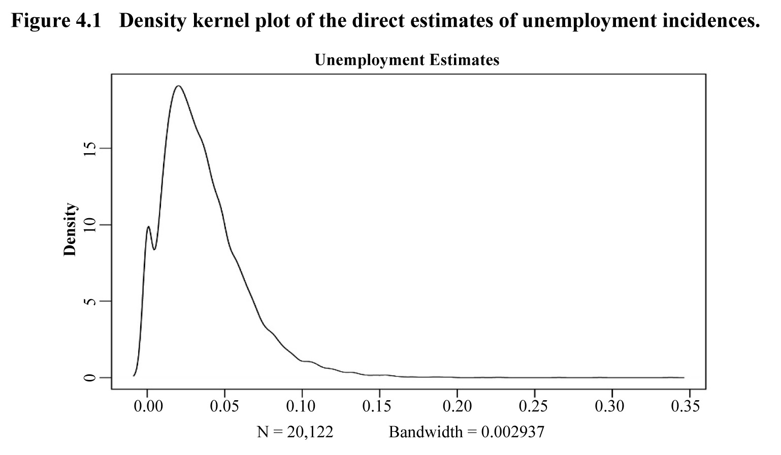
Description for Figure 4.1
Figure presenting a density kernel plot of the direct estimates of unemployment incidences (N = 20,122 and bandwidth = 0.002937). Density from 0 to 20 is on the y-axis and unemployment estimates from 0 to 0.35 are on the x-axis. The distribution is skewed with a right tail and a peak reached for an unemployment estimate of about 0.025.
The
model parameters of interest can be divided into three groups:
- the matrix of small area parameters:
- the vector of the measurement parameters:
- the set of latent parameters:
To
complete the Bayesian formulation of the proposed model, it is necessary to
choose priors for the model parameters. Small area parameters do not need a
specific prior because direct estimates based on observed data are available;
therefore, a set of priors is chosen for the measurement and the latent
parameters. Regarding
diffuse normal priors are assumed for the
regression coefficients. These priors are conjugate and computationally more
convenient than the usually flat priors over the real line (see Rao, 2003,
Chapter 10). In particular, we assume
with
and
is a known diagonal matrix.
Variances
are unknown and, therefore, it is necessary to
set a prior also on these parameters. The choice of the prior distribution for
the variance components is critical as in Bayesian mixed models the posterior
distributions of these parameters are known to be sensitive to this
specification. The inverse Gamma distribution is a popular choice, see e.g., You
et al. (2003) and Datta, Lahiri, Maiti and Lu (1999) among others. Gelman
(2006), Gelman, Jakulin, Pittau and Su (2008), and Polson and Scott (2012) propose
to assume a half-Cauchy distribution for the variance of the random effect.
Alternatively, a Uniform distribution can also be considered. Fabrizi
et al. (2016) conduct an exhaustive sensitivity analysis when using a
latent class model in a multivariate setting and find no significant difference
among these different alternatives. For this reason, we choose the same prior
distribution considered in You et al. (2003) and use an inverse Gamma
distribution with shape parameter
and scale parameter
then
where
are set to very small values. This choice
makes it also easier to derive the full conditional distributions for the Gibbs
sampler.
For
a system of Dirichlet priors is set on the
initial probabilities and on the transition probabilities. The Dirichlet
distribution is a conjugate prior for the multinomial distribution. This means
that if the prior distribution of the multinomial parameters is Dirichlet then
the posterior distribution belongs to the same family. The benefit of this choice
is that the posterior distribution is easy to compute and, in some sense, it is
possible to quantify how much our beliefs have changed after collecting the
data. Then, we assume
4.3 Estimation and model selection
In this work we make use of a
data augmentation Markov Chain Monte Carlo (MCMC) method (Tanner and Wong,
1987; Liu, Wong and Kong, 1994; Van Dyk and Meng, 2001) based on the Gibbs
sampler, in which the latent variables are treated as missing data (Marin et al.,
2005; Germain, 2010). There are two main reasons for this choice. First of all,
there is evidence that data augmentation has a better performance than other
methods, as the marginal updating scheme (Boys and Henderson, 2003). Moreover,
it simplifies the process of sampling from the posterior distribution. Details
on this method and the full conditionals employed in the Gibbs sampler are
given in Appendix A.1.
The choice of the number of
latent states is a crucial step in applications. In the framework of LMMs, this
requires a model selection procedure. From a Bayesian perspective, a
fundamental goal is the computation of the marginal likelihood of the data for
a given model. In this paper we use a model selection method based on the
marginal likelihood and to estimate this quantity we use the method proposed by
Carlin and Chib (1995), applied for each available model on the basis of the
output of the MCMC algorithm. Technical details are provided in Appendix A.2.
A well-known problem occurring
in Bayesian latent class and LMMs is the label switching. This implies that the
component parameters are not identifiable as they are exchangeable. In a
Bayesian context, if the prior distribution does not distinguish the component
parameters between each other, then the resulting posterior distribution will
be invariant with respect to permutations of the labels. Several solutions have
been proposed; for a general review see Jasra, Holmes and Stephens (2005). The
easiest approach is to use relabeling techniques retrospectively, by
post-processing the MCMC output (Marin et al., 2005). However, in our
case, we are interested in the prediction of the small area parameters, whose
distribution depends on the number of areas in each latent state. Therefore, we
do not use the post-processing approach and the MCMC output is permuted at
every iteration according to the ordering of the mean of the response variables
in each class.
