
Coordination of spatially balanced samples
Section 6. Application to Swiss establishments
We illustrate the application of the proposed methods on real data. The data that we used was collected by the Swiss Federal Statistical Office and can be downloaded for free (https://www.bfs.admin.ch/ bfs/fr/home/services/geostat/geodonnees-statistique-federale/etablissements-emplois/statistique-structurel-entreprises-statent-depuis-2011.assetdetail.3303058.html). It contains census data from 2013 and 2015 on Swiss establishments. Data for all establishments are aggregated at the hectare level. The geographical coordinates are proper to each hectare, and not to establishments. Each hectare can contain several establishments. The statistical unit was in this application an hectare, and not an establishment. We considered only hectares containing establishments from the economic activity 1 (agriculture, hunting, forestry, fisheries and aquaculture), and having in total at least 3 full-time equivalent employees. The years 2013 and 2015 were considered the two time occasions. In 2013, a number of 7,057 units were available, while in 2015 this number was 7,104. The overall population was of size 9,478. The difference in the sizes between the two time occasions was due to the 2,374 deaths and 2,421 births in 2015 compared to 2013. Figure 6.1 shows the geographical location of the units from the overall population. The parts inside of the figure with less locations correspond in majority to the Swiss Alps.
The data can be used with two main purposes:
- The location of each establishment in Switzerland has been geocoded since 1995. The register of establishments contains their geographical coordinates. Surveys are made to complete some missing information in this register. To achieve this, the Swiss Federal Statistical Office conducted such a survey in 2014. A positive coordination can be applied for example to check the quality of the the completed information from a time occasion to another one.
- Negative coordination can be applied to reduce the response burden of the establishments selected in several surveys. If the aggregated data are used, the hectares can be seen as primary selected units, while the establishments inside them as secondary units.
We used the values of the expected sample sizes 1,000 and 800, while and were computed proportional to the same variable measured in 2013 and 2015, respectively. This variables was the total number of full-time equivalent employees of all establishments inside of a hectar. A matrix of size of PRNs was generated for the LPM. For the other methods, the vector of PRNs was taken to be the main diagonal of this matrix. In both time occasions respectively, we selected samples and using Poisson sampling with PRNs, LPM with PRNs, SCPS with PRNs, TSCPS 1 with PRNs 0.25, 0.50, 0.75), and TSCPS 2 with PRNs 0.25, 0.50, 0.75). The Euclidean distance between locations was used in all methods, excepting Poisson sampling.
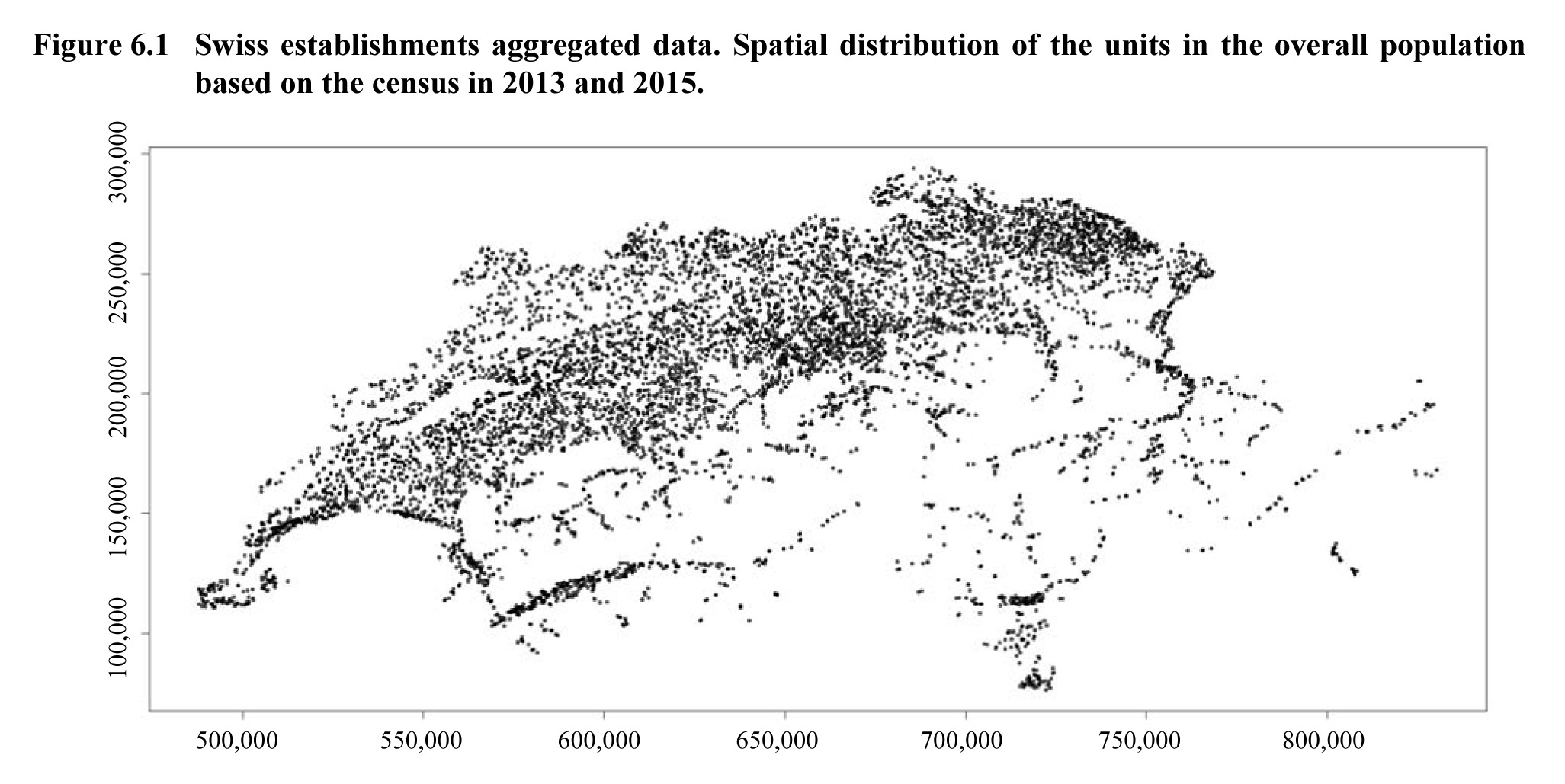
Description for Figure 6.1
Geographical map of Switzerland showing the spatial distribution of the units in the overall population based on the census in 2013 and 2015. Locations are less numerous in the Swiss Alps zone.
We analyzed the selected samples in terms of realised overlap and measure. To achieve this, positive and negative coordinations with PRNs were respectively applied. Table 6.1 shows the realised sample sizes as well as the overlap between different samples in both types of coordination. For the samples drawn in the first time occasion, the measure given in expression (3.3) is also indicated. Poisson sampling presents the highest overlap in positive coordination (560, when AUB = 538.022), while LPM the smallest one. Due to the important changes in the population from 2013 to 2015, SCPS performs better than LPM, with an overlap of 329, but worse than Poisson sampling. All the members of the TSCPS family perform intermediately between Poisson sampling and SCPS, in function of the value of Negative coordination shows the same superiority of Poisson sampling, while the other designs exhibit smaller values of the realised overlap, with SCPS performing again better than LPM. Moving now to the spatial balancing feature, Poisson sampling yields the largest realised measure, while LPM and SCPS as expected indicate the smallest ones. As in the results shown in Section 5.2, the members of the TSCPS family exhibit smaller realised measure than Poisson sampling, but larger than SCPS. The application of the proposed methods on these real data indicates similar behavior of them with the simulation results shown in Sections 5.1 and 5.2.
| Design | size of | Positive coord. | Negative coord. | ||||
|---|---|---|---|---|---|---|---|
| size of | overlap | size of | overlap | ||||
| Poisson | 1,010 | 840 | 560 | 779 | 46 | 0.387 | |
| LPM | 1,000 | 800 | 270 | 800 | 93 | 0.161 | |
| SCPS | 1,000 | 800 | 329 | 800 | 70 | 0.151 | |
| TSCPS 1 | 0.25 | 999 | 799 | 459 | 800 | 64 | 0.178 |
| 0.50 | 1,000 | 799 | 420 | 800 | 66 | 0.217 | |
| 0.75 | 1,000 | 800 | 366 | 800 | 67 | 0.178 | |
| TSCPS 2 | 0.25 | 1,012 | 830 | 469 | 808 | 49 | 0.275 |
| 0.50 | 1,020 | 828 | 409 | 799 | 58 | 0.194 | |
| 0.75 | 1,010 | 816 | 377 | 797 | 66 | 0.153 | |
- Date modified: