Bayes, buttressed by design-based ideas, is the best overarching paradigm for sample survey inference
Section 4. Examples
A variety of examples are offered, admittedly somewhat
slanted towards my own work with colleagues. I avoid topics such as small area
or time series estimation, because the need for modeling is well established
there.
Example 1 continued. Normal
random sample. A
common critique of model-based methods is “if I base an inference on a model
and the model is wrong, the inference must be wrong. Because (to paraphrase
George Box), all models are wrong, therefore all model-based inference is
wrong. So I prefer design-based inference, which does not require modeling
assumptions”. The reasoning is plausible but it’s not that simple. The validity
of model-based methods depends both on the design and on the degree and nature
of model misspecification; the fact that design-based methods do not overtly
depend on models does not mean they are necessarily superior to methods that
do.
Suppose a
simple random sample of size is taken from a continuous distribution with
unknown mean and standard deviation Consider three interval estimates for the population
mean:
- (i) Interval A is the standard
design-based 95% confidence interval, equation (3.1).
- (ii) Interval B replaces the 97.5th normal percentile in equation
(3.1), namely 1.96, by the 97.5th percentile of the distribution with df.
- (iii) Interval C is the 95%
posterior credible interval based on a normal model with the Jeffreys’ prior
distribution
From a
frequentist perspective, which of these intervals is the best? Interval A makes
no distributional assumption on and B makes a normal assumption does that mean that A is superior? If is large then the intervals are essentially the
same, and if is small then B is arguably better than A even
if the data are not normal, because it is reflecting uncertainty about the
variance.
In an informal
survey, two thirds of a recent class of our well-trained Ph.D. students
preferred B to C, on the grounds that it avoids the choice of prior
distribution and hence makes fewer assumptions. But B and C are equally good or
bad, because they are the same procedure! That this interval is an exact 95%
confidence interval under normality, and is a 95% credible interval for the
stated choice of prior, are just two properties of the procedure. Judging a
method by its overt assumptions is an over-simplification.
Example 2. Simple random
sample with a lower bound on the variance (Little, 2006). Suppose in the previous
example that The standard interval (ignoring finite population
corrections) is
if in fact we know that 1.5, a better interval is
the wider interval reflecting
the fact that is greater than the particular value of for this sample. The t interval (4.1) has
exact confidence coverage, but, given what we know about it is the wrong inference for this specific
data set: we should not pick it over (4.2) because it is narrower!
Now suppose we
know that 1.5, because of some unaccounted
source of additional variation. The Bayesian approach then incorporates this
information into the prior distribution for resulting in a credible interval that is wider
than (4.2). What is the frequentist answer? The t confidence interval still has
exactly nominal coverage in repeated sampling, but it is clearly too narrow as
an inference for the observed dataset, because it fails to reflect what is
known about The interval (4.2) is anticonservative,
despite the fact that it is wider than (4.1) for the realized data set a property that can happen for confidence
intervals but cannot happen for credible intervals under a specific model.
Asymptotic frequentist methods are no help here, so what is the alternative to
Bayes in this example?
A related
example arises in one group random-effects analysis of variance, when the least
squares estimate of the between-group variance is negative a Bayesian analysis addresses this with a
prior distribution on the between-group variance that does not allow negative
values. Random-effects and mixed-effects models are important to handle
clustering in surveys, and Bayesian methods are better than ML in this setting.
Example 3. Post-stratification
on a categorical covariate. Prediction (as in modeling) is a more reliable general
approach to inference than weighting (as in design-based inference). I
illustrate this general statement with the simple example of
post-stratification on a single variable A more complex example Example 7 is given later.
Consider an
equal probability sample with a single categorical post-stratifying variable for which known population counts are available for each post-stratum Let be the sample mean in post-stratum based on sample size and The standard estimate of the population mean is the
post-stratified mean:
where and is
the population size. This can be viewed as a weighted mean
where is the post-stratification weight for sampled
units in poststratum These weights can be very large in post-strata
with small sample sizes which, unlike stratified sampling based on are not under the control of the sampler.
These large weights can lead to excessive variability in In fact, strictly speaking, does not have a distribution in repeated
sampling, because with positive probability the sample sizes in some
post-strata may be zero. This remains true if the post-strata are modified to
ensure that the post-strata sample counts are all positive for the observed
sample, for example by pooling adjacent strata.
The standard
design-based approach to excessive variability of is to modify the weights for example by trimming the large ones.
However, from a prediction perspective, this is misguided. The problem is not
the weights the population proportions in each post-stratum are known, after all the problem is that sparsity of sample in some
post-strata renders the estimates unreliable. It is the estimates in sparse
post-strata that need to be modified, not the weights attached to sampled units. The principled way
to modify is to assume a model relating and The design-based approach, by avoiding such a
model, leads to the wrong principle modifying the weights rather than the predictions
of non-sampled values.
A related
point: a common design-based approximation (Kish, 1992) measures the
proportionate increase in variance from weighting as where is the coefficient of variation of the
weights; trimming the weights reduces and hence this proportionate increase.
However, this rule of thumb is only valid when and are unrelated, in which case
post-stratification is useless. If and are related and the sample size is not too
small, the variance of the post-stratified mean is smaller, not larger,
than the variance of the unweighted sample mean (Holt and Smith, 1979; Little
and Vartivarian, 2005). The rule of thumb fails because the relationship
between and is not modeled.
What is the
Bayesian approach to excessive variability of The latter is the posterior mean for the
stratified normal model
where denotes the normal (Gaussian) distribution with
mean variance and equation (4.5) is the Jeffreys’ prior
distribution on the mean and standard deviation in each post-stratum. Given a
sparse sample in some post-strata, the prior distribution needs to be modified
to allow borrowing of strength from other strata. One approach is to assume the
normal random-effects model
which treats the stratum means
as random effects. The variances in each post-stratum might also be treated as
distinct random effects and assigned a prior distribution, rather than pooled.
The posterior mean of for the prior distribution (4.6) moves the
weight of sampled units in post-stratum towards one, with a degree of shrinkage that
depends on the relative size of estimates of and (Lazzeroni and Little, 1998).
The prior
distribution (4.6) makes the non-trivial assumption that the post-stratum means
are exchangeable. It can be relaxed by restricting the random effects model to
a subset of post-strata with small sample counts; or the constant mean in (4.6) might be replaced by a regression on
known post-stratum characteristics as in:
which limits the
exchangeability assumption to the errors in the regression of on For extensive generalizations of this basic
example, see Gelman and Little (1997), Elliott and Little (2000), Elliott
(2007), Gelman (2007) and Si,
Trangucci, Gabry and Gelman (2020).
Example 4. Regression
estimator of the mean, given a population auxiliary variable. If the auxiliary variable in the previous example is continuous, a
common way to incorporate it in the inference is via the regression estimate of
the mean:
where is the least squares estimate of the slope of on in the sample, and and are respectively the sample and population
mean of In a simulation study of five real
populations, Royall and Cumberland (1981, 1985) assess inferences centered at with (a) the standard design-based standard
error based on simple random sampling, namely:
where is the sample residual variance and is the sampling fraction; and (b) the
prediction standard error based on the normal linear regression model with
constant variance, namely:
The
design-based confidence intervals exhibit very poor conditional confidence
coverage when the observed deviates substantially from The model-based confidence interval takes into account this lack
of balance with respect to but is vulnerable to model misspecification,
specifically lack of linearity in the relationship between and or non-constant residual variance. Robust
estimates of standard error, based on the sandwich estimator or the jackknife,
yield intervals with better conditional coverage properties, although still
sometimes deviating from nominal coverage levels. An alternative approach is
Bayesian inference based on a more flexible model relating to such as the penalized spline model:
where the constants are selected fixed knots, and if and 0, otherwise (see, for example Ruppert,
Wand and Carroll, 2003). The
parameter allows for a variety of common forms of
heteroskedasticity. The Bayesian standard errors then reflect imbalance in
distribution of in the sample and population, and the
flexibility of the model limits bias from model misspecification.
Suppose that
the target quantity is not the population mean of but the least squares slope of on in the population. A robust approach is to
impute the non-sampled values of using the model (4.8), and then estimate the
slope of on as the least squares slope estimated on the
filled-in population data. Uncertainty can be propagated by multiple imputation
(Rubin, 1987), a method founded on Bayesian ideas. In this context, Little
(2004) distinguishes between the “target model” that determines the target
population quantity of interest, here the linear regression of on and the “working model” (4.8) that is the
basis for inference, and is used to predict survey variables for the non-sampled
and nonresponding units in the population. Distinguishing between these two
models provides for a robust form of Bayesian survey inference.
Szpiro, Rice
and Lumley (2010) apply a similar idea in a superpopulation regression setting,
and Little (2019) argues that this is more straightforward than changing the
interpretation of the estimand, the approach adopted by Buja, Berk, Brown, George, Pitkin, Zhan and
Zhang (2019).
Szpiro et al. (2010) show that the approach provides a Bayesian
interpretation of the sandwich estimator of variance in regression, which is
asymptotically equivalent to sample reuse estimates of variance like the
bootstrap or jackknife, which are commonly applied in sample survey settings.
Example 5. Inference for
samples with unequal probabilities of selection. For designs with unequal
selection probabilities, classic papers critiquing the modeling approach to
surveys (Kish and Frankel, 1974; Hansen, Madow and Tepping, 1983) do not
include the selection probabilities in the model, yielding inferences that are
vulnerable to model misspecification. The selection probabilities play an
important role in robust model-based inference, but as model covariates rather
than as sampling weights.
Consider, for
example, inference about a population mean If is the value of a survey variable and is the selection probability for unit the usual design-based estimator of the mean
of weights sampled units (say units by the inverse of resulting in the Horvitz-Thompson estimate
(Horvitz and Thompson, 1952)
if the population size is
known, or the Hájek (1971) estimate
if is estimated. Weighting is a “one size fits
all” approach, with sampled units receiving the same weight irrespective of the
relationship between and This is potentially inefficient if the relationship is weak, weighting simply
reduces the precision of the estimate without a compensating reduction in bias.
The modeling
approach incorporates the selection probabilities by regressing on The strength of relationship between and then moderates how the selection probability
affects the estimator if the relationship is weak, the regression
coefficient of is small and the sampling weight has little
influence. This results in more efficient estimates.
A linear
regression of on is vulnerable to bias if the linearity is
misspecified, but the impact of misspecification can be reduced by choosing a
model that results in a design-consistent estimate. Many models satisfy this
requirement; see for example Firth and Bennett (1998).
In stratified
sampling with stratifying variable the natural regression model includes
covariates that are dummy variables for the strata. The resulting estimate of
the population mean of a continuous survey variable is the stratified mean, which has the same
form as equation (4.3) but with forming strata rather than post-strata.
Weighting by the inverse of the selection probability in each stratum and dummy
variable regression both yield the estimator (4.3) in this situation. The
Bayesian approaches to reducing variance described in example 3 tend to have
less pay-off in the case of stratified sampling than for post-stratification,
because the sampler has control over the sample sizes in each stratum.
In probability
proportional to size (PPS) sampling, the covariate is the size of the unit and Now is a continuous variable, and weighting and
regression may yield different answers. The approaches can be unified by
considering models that yield the design-weighted estimates when used to
predict the non-sampled units. In particular, ignoring finite population corrections,
the HT estimate (4.9) is the posterior mean for the “Horvitz Thompson model”:
and the Hájek estimate (4.10)
is the posterior mean for the “Hájek model”:
These
underlying models describe situations where the corresponding design-based
estimates are optimal. However, they involve strong parametric assumptions. A
robust Bayesian modeling approach embeds these models within a larger model,
such as the penalized spline model (4.8), as proposed by Zheng and Little
(2003). Zheng and Little (2005) and Chen,
Elliott, Haziza, Yang, Ghosh, Little, Sedransk and Thompson (2017) provide simulation
studies suggesting that this modeling approach can yield substantial gains over
HT or Hájek estimation, both in terms of efficiency and closer to nominal
(frequentist) confidence coverage in moderate samples remember, design-based results are asymptotic.
The model (4.8) is readily expanded to include other auxiliary variables
measured for all the population units, and the flexibility of small-sample
inferences increased by including proper prior distributions for the model
parameters.
Leon-Novelo and
Savitsky (2019) consider Bayesian models for the joint distribution of and calling models that fix a “plug-in” approach. However, assigning a
distribution to seems to me both unnatural and unnecessary in
this setting; if is recorded for all population units, it can
be conditioned in the model, as in standard regression approaches that treat
covariates as fixed. Even if values of for non-sampled units are not provided to
analysts, their values can be predicted via Bayes Theorem, as in Zangeneh and
Little (2015).
Example 6. Penalized spline of
response propensity models. Consider unit nonresponse on a survey variable when a set of variables say are observed for respondents and
nonrespondents in the sample. The response propensity for unit where represents unknown parameters, plays an
important role in both weighting and prediction approaches to survey
nonresponse. In nonresponse weighting the sampling weight is multiplied by the
nonresponse weight, as in
Unlike the
sampling weight, the response weight is unknown, and the definition needs to be
clear on what the probability is conditioned. Little (2022) argues that it
should condition on auxiliary and survey variables, but not on other variables
that might affect it. As with sampling weights, weighting by the inverse of the
estimated response propensity is a “one size fits all” approach that does not
take into account the strength of relationship between and Penalized Spline of Propensity Prediction
(PSPP, Zhang and Little, 2009) regresses on a penalized spline of the estimated response
propensity, with other variables that are observed for respondents and
nonrespondents entering parametrically. The spline models a flexible
relationship between the response propensity and providing robustness to model
misspecification. The balancing property of the propensity score also provides
a double robustness property, in that the parametric form of the regression on
other predictors can be misspecified without bias, provided the penalized
spline captures the relationship between the propensity and This method performs favorably with weighting
methods in simulations (Zhang and Little, 2009; Yang and Little, 2015), and the
fully Bayes version with prior distributions on the parameters propagates error
in estimating the propensities.
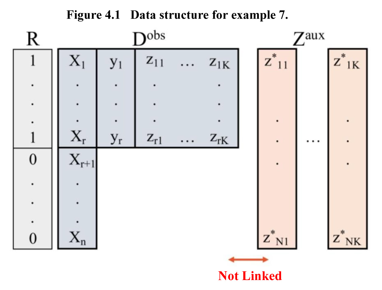
Description of Figure 4.1
Figure representing the data
structure for the data set of example 7. is a survey variable subject to nonresponse The set of observations contains data for units, of which are respondents and are non-respondents. is a variable observed forall units in the
sample, and consists of a set of categorical auxiliary
variables only observed for the respondents. The joint distribution of is observed for survey respondents, and the
marginal distributions of are also observed for the population or sample
from external sources. A distinctive feature is that the units in the auxiliary
data are not linked with the units in the survey.
Example 7. Unit nonresponse with
poststratification. Another example where Bayesian and design-based approaches to inference
differ concerns unit nonresponse with post-stratification. Consider the setting
of Figure 4.1, where is a survey variable subject to nonresponse, is a variable observed for all units in the
sample, and consists of a set of categorical auxiliary
variables. The joint distribution of is observed for survey respondents, and the marginal
distributions of are also observed for the population or sample
from external sources. A distinctive feature is that the units in the auxiliary
data are not linked with the units in the survey. This scenario occurs
frequently in settings where post-stratification is used for nonresponse
adjustment. Define as the response indicator for for sample unit and suppose that
so that this probability does
not depend on Note that if this probability depends on the response mechanism is missing not at
random (MNAR) according to Rubin’s (1976) definition, because values of are missing for survey nonrespondents.
Zangeneh and Little (2022) consider Bayes and ML estimation for data with this
pattern. Considering for simplicity models that are i.i.d. over the units the joint distribution of and is factored as
where and are distinct parameters (Little and Rubin,
2019, Chapter 6). The parameters in this factorization can thus be estimated
from the respondent survey data with and parameters of the joint distribution of and are estimated by combining the respondent and
auxiliary data on those variables.
Two special
cases considered by Zangeneh and Little (2022) are as follows:
- No covariates
and a single post-stratifier The missingness assumption in equation (4.13)
then reduces to The parameters of the conditional distribution
of given are estimated from the survey respondents, and
the parameters of the marginal distribution of are estimated from the auxiliary data on In particular, if is multinomial with the ML estimate of is simply the proportion of the auxiliary
counts in post-stratum If, in addition, given is assumed normal with mean and variance the resulting ML estimate of the population
mean of is simply the post-stratified mean given in equation
(4.3). This simple example is interesting theoretically, because the response
mechanism is MNAR but ignorable for likelihood inference; MAR is a sufficient
but not always necessary condition for ignorability.
- is a
single categorical variable and is a single categorical post-stratifier. Now the
joint distribution of and is not identified under a saturated model, and
requires additional assumptions to identify the model. In particular, a constrained
MNAR “RAKE” model assumes that the marginal distributions of and are different for respondents and
nonrespondents, but the odds ratios of and are the same for respondents and
nonrespondents. This yields a just-identified model. Raking the table of
respondent counts of and to the auxiliary margins of and yields ML estimates of under this RAKE model. (Little and Wu, 1991;
Little, 1993). The post-stratified estimator of the mean of is then
where is the proportion of the population with from raking the respondent counts to the
margins, and is the estimated mean of given from the model for given and
Some comments
on this approach are as follows:
- Note again this is a MNAR model, and it is
weaker than the MAR model that assumes that response depends on but not on As a result, the method tends to be less
biased than alternative methods that assume MAR for consistent estimates.
- As was the case in example 4, the ML approach
to this model does not involve modifying the weights applied to the data in
cell using arbitrary distance functions the ML estimates are fully efficient under the
assumed model.
- Sparse data in the cells can be addressed by
adding proper prior distributions for the parameters and applying Bayesian
methods. For example, for inference about the parameters of the distribution of given one might assume a flat prior on the main
effects of and but a normal prior on the interactions,
shrinking them towards zero. This achieves shrinkage of the cell mean towards the fitted means from an additive
model. In frequentist terminology, this is a mixed ANOVA model with fixed main
effects and random interactions.
- The idea of raking to the and margins is familiar, but note that if is a stratifier and is a post-stratifier, the standard approach is
to perform one iteration of raking, first matching the margin and then matching the margin: under the assumed model, raking
iteratively is the correct procedure. Raking is ML here, but Bayesian forms of
raking also can be used to propagate parameter uncertainty.
Example 8. Proxy pattern-mixture
analysis. Proxy
pattern-mixture analysis is a method for assessing nonresponse bias for the
mean of a survey variable subject to nonresponse, when there is a set of
covariates observed for nonrespondents and respondents. Historically the amount
of missing data, as measured by the response rate, has been the most often-used
metric for evaluating survey quality. However, response rates ignore the
information contained in auxiliary covariates observed for nonrespondents.
Methods based on the estimated probability of nonresponse such as the R
indicator (Schouten, Cobben and Bethlehem, 2009) and q2 measure (Särndal and
Lundström, 2010) do not take into account the strength of association of the
survey variable of interest and the probability of response, which arguably
should be factored into the assessment of bias. These measures assume MAR, but
if the auxiliary variables are available for nonresponse adjustment, it is
deviations from MAR that lead to bias.
Andridge and
Little (2011) propose proxy pattern-mixture analysis (PPMA), a method based on
a pattern-mixture model for nonresponse that combines in a simple and intuitive
way the key features of nonresponse adjustment. Let denote the value of a continuous survey
outcome and denote the values of covariates for unit in the sample. Only of the sampled units respond, so observed data
consist of for and for Let denote the response indicator, such that for
unit if is observed and if is missing. To reduce dimensionality, we
replace by a single proxy variable that has the highest correlation with in the respondent sample. This proxy variable can be
estimated by regressing on using the respondent data, including important
predictors of as well as interactions and nonlinear terms
where appropriate. Specifically, we assume the regression model and let The joint distribution of and using the following proxy pattern-mixture
model, similar in form to that discussed in Little (1994):
where denotes the bivariate normal distribution. Our
interest is bias in the marginal mean of which can be written as Andridge and Little (2011) assume that
for some unspecified function and known constant Here is the proxy scaled to have the same variance as which aids the interpretation of by putting and on the same scale. This mechanism is MAR when and deviates increasingly from MAR as increases. With this assumption, the
parameters are just identified and the ML estimate of the mean of averaging over patterns, is
where are the respondent means of and and is the mean of for nonrespondents. The index of bias is then
the adjustment of the sample mean implied by this estimate, namely
where is the respondent sample correlation. This
adjustment incorporates three key factors that affect the potential bias in a
simple and intuitive manner the nonresponse rate the correlation between and and the deviation of from In particular, the index increases with the
nonresponse rate and the deviation of the mean of for respondents and nonrespondents.
There is no
information about the parameter in the data this is generally the case for methods that model
deviations from MAR. Following Little (1994), Andridge and Little (2011) propose
a sensitivity analysis, where estimates are generated for a range of values of between 0 and infinity, specifically 0, 1 and
infinity; the choice of 0 corresponds to MAR, the intermediate choice of 1
implies the bias of is the same as the bias of the proxy variable and the choice of infinity is the most extreme
deviation from MAR; estimates for this case have the highest variance. As varies between 0 and infinity, the middle
factor varies between (when is the standard regression estimator of the
mean) and (when is the inverse regression estimator proposed
by Brown (1990). The sensitivity of the estimate to the choice of is small when is close to 1, that is we have a strong proxy
variable, and large when is close to 0, that is we have a weak proxy
variable. So having auxiliary variables that are good predictors of the survey
outcomes is crucial.
Bayesian
versions of the proxy pattern-mixture model are readily developed, allowing for
propagation of error in the model parameters. Also, the model can be applied to
create multiple imputations of nonrespondent values, allowing the incorporation
of complex sample design elements into the index.
More recently,
the model has been used to develop indices of departure from random sampling,
by applying it to model selection rather than nonresponse (Little, West,
Boonstra and Hu, 2020; Boonstra, Little, West, Andridge and Alvaredo-Leiton, 2021).
Refinements in this work are (a) to replace the parameter by a better parametrization because ranges from 0 (MAR) to 1, and (b) (with some
additional assumptions) to allow missingness also to depend on auxiliary
variables orthogonal to The method has also been extended to handle
binary outcomes (Andridge, West, Little, Boonstra and Alvarado-Leiton, 2019)
and indices of potential bias in regression coefficients (West, Little, Andridge, Boonstra, Ware, Pandit
and Alvarado-Leiton, 2021).
