Multiple-frame surveys for a multiple-data-source world
Section 4. Multiple-frame surveys and data integration

Rao (2021) reviewed a number of data integration methods for combining information from a probability sample S 1 , MathType@MTEF@5@5@+= feaagKart1ev2aaatCvAUfeBSjuyZL2yd9gzLbvyNv2CaerbuLwBLn hiov2DGi1BTfMBaeXatLxBI9gBaerbd9wDYLwzYbItLDharqqtubsr 4rNCHbGeaGqiFu0Je9sqqrpepC0xbbL8F4rqqrFfpu0de9LqFHe9Lq pepeea0xd9q8as0=LqLs=Jirpepeea0=as0Fb9pgea0lrP0xe9Fve9 Fve9qapdbaqaaeGaciGaaiaabeqaamaabaabaaGcbaGaam4uamaaBa aaleaacaaIXaaabeaakiaacYcaaaa@3A8E@ assumed to come from a frame with complete coverage, with information from a nonprobability sample S 2 , MathType@MTEF@5@5@+= feaagKart1ev2aqatCvAUfeBSjuyZL2yd9gzLbvyNv2CaerbuLwBLn hiov2DGi1BTfMBaeXatLxBI9gBaerbd9wDYLwzYbItLDharqqtubsr 4rNCHbGeaGqiFu0Je9sqqrpepC0xbbL8F4rqqrFfpu0de9LqFHe9Lq pepeea0xd9q8as0=LqLs=Jirpepeea0=as0Fb9pgea0lrP0xe9Fve9 Fve9qapdbaqaaeGaciGaaiaabeqaamaabaabaaGcbaGaam4uamaaBa aaleaacaaIYaaabeaakiaacYcaaaa@3A90@ often a census of part of the population as in Section 3.4. Rao considered two cases for making inferences about y MathType@MTEF@5@5@+= feaagKart1ev2aqatCvAUfeBSjuyZL2yd9gzLbvyNv2CaerbuLwBLn hiov2DGi1BTfMBaeXatLxBI9gBaerbd9wDYLwzYbItLDharqqtubsr 4rNCHbGeaGqiFu0Je9sqqrpepC0xbbL8F4rqqrFfpu0de9LqFHe9Lq pepeea0xd9q8as0=LqLs=Jirpepeea0=as0Fb9pgea0lrP0xe9Fve9 Fve9qapdbaqaaeGaciGaaiaabeqaamaabaabaaGcbaGaamyEaiaacQ daaaa@39D2@ : (1) y MathType@MTEF@5@5@+= feaagKart1ev2aqatCvAUfeBSjuyZL2yd9gzLbvyNv2CaerbuLwBLn hiov2DGi1BTfMBaeXatLxBI9gBaerbd9wDYLwzYbItLDharqqtubsr 4rNCHbGeaGqiFu0Je9sqqrpepC0xbbL8F4rqqrFfpu0de9LqFHe9Lq pepeea0xd9q8as0=LqLs=Jirpepeea0=as0Fb9pgea0lrP0xe9Fve9 Fve9qapdbaqaaeGaciGaaiaabeqaamaabaabaaGcbaGaamyEaaaa@3914@ is observed in both samples, and (2) auxiliary information x MathType@MTEF@5@5@+= feaagKart1ev2aqatCvAUfeBSjuyZL2yd9gzLbvyNv2CaerbuLwBLn hiov2DGi1BTfMBaeXatLxBI9gBaerbd9wDYLwzYbItLDharqqtubsr 4rNCHbGeaGqiFu0Je9sqqrpepC0xbbL8F4rqqrFfpu0de9LqFHe9Lq pepeea0xd9q8as0=LqLs=Jirpepeea0=as0Fb9pgea0lrP0xe9Fve9 Fve9qapdbaqaaeGaciGaaiaabeqaamaabaabaaGcbaGaaCiEaaaa@3917@ is observed in both samples but y MathType@MTEF@5@5@+= feaagKart1ev2aqatCvAUfeBSjuyZL2yd9gzLbvyNv2CaerbuLwBLn hiov2DGi1BTfMBaeXatLxBI9gBaerbd9wDYLwzYbItLDharqqtubsr 4rNCHbGeaGqiFu0Je9sqqrpepC0xbbL8F4rqqrFfpu0de9LqFHe9Lq pepeea0xd9q8as0=LqLs=Jirpepeea0=as0Fb9pgea0lrP0xe9Fve9 Fve9qapdbaqaaeGaciGaaiaabeqaamaabaabaaGcbaGaamyEaaaa@3914@ is observed only in S 2 . MathType@MTEF@5@5@+= feaagKart1ev2aqatCvAUfeBSjuyZL2yd9gzLbvyNv2CaerbuLwBLn hiov2DGi1BTfMBaeXatLxBI9gBaerbd9wDYLwzYbItLDharqqtubsr 4rNCHbGeaGqiFu0Je9sqqrpepC0xbbL8F4rqqrFfpu0de9LqFHe9Lq pepeea0xd9q8as0=LqLs=Jirpepeea0=as0Fb9pgea0lrP0xe9Fve9 Fve9qapdbaqaaeGaciGaaiaabeqaamaabaabaaGcbaGaam4uamaaBa aaleaacaaIYaaabeaakiaac6caaaa@3A92@ In this section I examine various data integration methods from the perspective of the multiple-frame paradigm and the assumptions in Section 2.2.

4.1   Small area estimation

Small area estimation can be considered to be a special case of a dual-frame estimation problem in which Assumption (A6) is not met. Here, S 1 MathType@MTEF@5@5@+= feaagKart1ev2aqatCvAUfeBSjuyZL2yd9gzLbvyNv2CaerbuLwBLn hiov2DGi1BTfMBaeXatLxBI9gBaerbd9wDYLwzYbItLDharqqtubsr 4rNCHbGeaGqiFu0Je9sqqrpepC0xbbL8F4rqqrFfpu0de9LqFHe9Lq pepeea0xd9q8as0=LqLs=Jirpepeea0=as0Fb9pgea0lrP0xe9Fve9 Fve9qapdbaqaaeGaciGaaiaabeqaamaabaabaaGcbaGaam4uamaaBa aaleaacaaIXaaabeaaaaa@39D5@ is a probability sample from Frame 1 and Frame 2 is often an administrative data source. Both frames are assumed to have complete coverage of the population, but the variable of interest y MathType@MTEF@5@5@+= feaagKart1ev2aqatCvAUfeBSjuyZL2yd9gzLbvyNv2CaerbuLwBLn hiov2DGi1BTfMBaeXatLxBI9gBaerbd9wDYLwzYbItLDharqqtubsr 4rNCHbGeaGqiFu0Je9sqqrpepC0xbbL8F4rqqrFfpu0de9LqFHe9Lq pepeea0xd9q8as0=LqLs=Jirpepeea0=as0Fb9pgea0lrP0xe9Fve9 Fve9qapdbaqaaeGaciGaaiaabeqaamaabaabaaGcbaGaamyEaaaa@3914@ is measured only in S 1 . MathType@MTEF@5@5@+= feaagKart1ev2aqatCvAUfeBSjuyZL2yd9gzLbvyNv2CaerbuLwBLn hiov2DGi1BTfMBaeXatLxBI9gBaerbd9wDYLwzYbItLDharqqtubsr 4rNCHbGeaGqiFu0Je9sqqrpepC0xbbL8F4rqqrFfpu0de9LqFHe9Lq pepeea0xd9q8as0=LqLs=Jirpepeea0=as0Fb9pgea0lrP0xe9Fve9 Fve9qapdbaqaaeGaciGaaiaabeqaamaabaabaaGcbaGaam4uamaaBa aaleaacaaIXaaabeaakiaac6caaaa@3A91@ Auxiliary information x MathType@MTEF@5@5@+= feaagKart1ev2aqatCvAUfeBSjuyZL2yd9gzLbvyNv2CaerbuLwBLn hiov2DGi1BTfMBaeXatLxBI9gBaerbd9wDYLwzYbItLDharqqtubsr 4rNCHbGeaGqiFu0Je9sqqrpepC0xbbL8F4rqqrFfpu0de9LqFHe9Lq pepeea0xd9q8as0=LqLs=Jirpepeea0=as0Fb9pgea0lrP0xe9Fve9 Fve9qapdbaqaaeGaciGaaiaabeqaamaabaabaaGcbaGaaCiEaaaa@3917@ used to predict y MathType@MTEF@5@5@+= feaagKart1ev2aqatCvAUfeBSjuyZL2yd9gzLbvyNv2CaerbuLwBLn hiov2DGi1BTfMBaeXatLxBI9gBaerbd9wDYLwzYbItLDharqqtubsr 4rNCHbGeaGqiFu0Je9sqqrpepC0xbbL8F4rqqrFfpu0de9LqFHe9Lq pepeea0xd9q8as0=LqLs=Jirpepeea0=as0Fb9pgea0lrP0xe9Fve9 Fve9qapdbaqaaeGaciGaaiaabeqaamaabaabaaGcbaGaamyEaaaa@3914@ is measured in both samples. Beaumont and Rao (2021) discussed integrating probability and nonprobability samples through the use of the Fay-Herriot (1979) estimator with small area estimation techniques.

A composite small area estimator (Rao and Molina, 2015) of the population mean η a MathType@MTEF@5@5@+= feaagKart1ev2aqatCvAUfeBSjuyZL2yd9gzLbvyNv2CaerbuLwBLn hiov2DGi1BTfMBaeXatLxBI9gBaerbd9wDYLwzYbItLDharqqtubsr 4rNCHbGeaGqiFu0Je9sqqrpepC0xbbL8F4rqqrFfpu0de9LqFHe9Lq pepeea0xd9q8as0=LqLs=Jirpepeea0=as0Fb9pgea0lrP0xe9Fve9 Fve9qapdbaqaaeGaciGaaiaabeqaamaabaabaaGcbaGaeq4TdG2aaS baaSqaaiaadggaaeqaaaaa@3AD4@ in area a MathType@MTEF@5@5@+= feaagKart1ev2aqatCvAUfeBSjuyZL2yd9gzLbvyNv2CaerbuLwBLn hiov2DGi1BTfMBaeXatLxBI9gBaerbd9wDYLwzYbItLDharqqtubsr 4rNCHbGeaGqiFu0Je9sqqrpepC0xbbL8F4rqqrFfpu0de9LqFHe9Lq pepeea0xd9q8as0=LqLs=Jirpepeea0=as0Fb9pgea0lrP0xe9Fve9 Fve9qapdbaqaaeGaciGaaiaabeqaamaabaabaaGcbaGaamyyaaaa@38FC@ is of the form

η ^ a = θ a η ^ a ( 1 ) + ( 1 θ a ) η ^ a ( 2 ) , MathType@MTEF@5@5@+= feaagKart1ev2aaatCvAUfeBSjuyZL2yd9gzLbvyNv2CaerbuLwBLn hiov2DGi1BTfMBaeXatLxBI9gBaerbd9wDYLwzYbItLDharqqtubsr 4rNCHbGeaGqiFu0Je9sqqrpepC0xbbL8F4rqqrFfpu0de9LqFHe9Lq pepeea0xd9q8as0=LqLs=Jirpepeea0=as0Fb9pgea0lrP0xe9Fve9 Fve9qapdbaqaaeGaciGaaiaabeqaamaabaabaaGcbaGafq4TdGMbaK aadaWgaaWcbaGaamyyaaqabaGccaaMe8UaaGypaiaaysW7cqaH4oqC daWgaaWcbaGaamyyaaqabaGccuaH3oaAgaqcamaaDaaaleaacaWGHb aabaGaaGikaiaaigdacaaIPaaaaOGaaGjbVlabgUcaRiaaysW7caaI OaGaaGymaiaaysW7cqGHsislcaaMe8UaeqiUde3aaSbaaSqaaiaadg gaaeqaaOGaaGykaiaaysW7cuaH3oaAgaqcamaaDaaaleaacaWGHbaa baGaaGikaiaaikdacaaIPaaaaOGaaGilaaaa@5ACB@

where η ^ a ( 1 ) MathType@MTEF@5@5@+= feaagKart1ev2aqatCvAUfeBSjuyZL2yd9gzLbvyNv2CaerbuLwBLn hiov2DGi1BTfMBaeXatLxBI9gBaerbd9wDYLwzYbItLDharqqtubsr 4rNCHbGeaGqiFu0Je9sqqrpepC0xbbL8F4rqqrFfpu0de9LqFHe9Lq pepeea0xd9q8as0=LqLs=Jirpepeea0=as0Fb9pgea0lrP0xe9Fve9 Fve9qapdbaqaaeGaciGaaiaabeqaamaabaabaaGcbaGafq4TdGMbaK aadaqhaaWcbaGaamyyaaqaaiaaiIcacaaIXaGaaGykaaaaaaa@3D05@ is the direct estimator for the sample mean in area a MathType@MTEF@5@5@+= feaagKart1ev2aqatCvAUfeBSjuyZL2yd9gzLbvyNv2CaerbuLwBLn hiov2DGi1BTfMBaeXatLxBI9gBaerbd9wDYLwzYbItLDharqqtubsr 4rNCHbGeaGqiFu0Je9sqqrpepC0xbbL8F4rqqrFfpu0de9LqFHe9Lq pepeea0xd9q8as0=LqLs=Jirpepeea0=as0Fb9pgea0lrP0xe9Fve9 Fve9qapdbaqaaeGaciGaaiaabeqaamaabaabaaGcbaGaamyyaaaa@38FC@ from S 1 MathType@MTEF@5@5@+= feaagKart1ev2aqatCvAUfeBSjuyZL2yd9gzLbvyNv2CaerbuLwBLn hiov2DGi1BTfMBaeXatLxBI9gBaerbd9wDYLwzYbItLDharqqtubsr 4rNCHbGeaGqiFu0Je9sqqrpepC0xbbL8F4rqqrFfpu0de9LqFHe9Lq pepeea0xd9q8as0=LqLs=Jirpepeea0=as0Fb9pgea0lrP0xe9Fve9 Fve9qapdbaqaaeGaciGaaiaabeqaamaabaabaaGcbaGaam4uamaaBa aaleaacaaIXaaabeaaaaa@39D5@ (which may have large variance or may not exist), η ^ a ( 2 ) = x a T β ^ MathType@MTEF@5@5@+= feaagKart1ev2aqatCvAUfeBSjuyZL2yd9gzLbvyNv2CaerbuLwBLn hiov2DGi1BTfMBaeXatLxBI9gBaerbd9wDYLwzYbItLDharqqtubsr 4rNCHbGeaGqiFu0Je9sqqrpepC0xbbL8F4rqqrFfpu0de9LqFHe9Lq pepeea0xd9q8as0=LqLs=Jirpepeea0=as0Fb9pgea0lrP0xe9Fve9 Fve9qapdbaqaaeGaciGaaiaabeqaamaabaabaaGcbaGafq4TdGMbaK aadaqhaaWcbaGaamyyaaqaaiaaiIcacaaIYaGaaGykaaaakiaaysW7 caaI9aGaaGjbVlaahIhadaqhaaWcbaGaamyyaaqaaiaadsfaaaGcca aMc8UabCOSdyaajaaaaa@46C1@ is a predicted value from a regression model, and θ a MathType@MTEF@5@5@+= feaagKart1ev2aqatCvAUfeBSjuyZL2yd9gzLbvyNv2CaerbuLwBLn hiov2DGi1BTfMBaeXatLxBI9gBaerbd9wDYLwzYbItLDharqqtubsr 4rNCHbGeaGqiFu0Je9sqqrpepC0xbbL8F4rqqrFfpu0de9LqFHe9Lq pepeea0xd9q8as0=LqLs=Jirpepeea0=as0Fb9pgea0lrP0xe9Fve9 Fve9qapdbaqaaeGaciGaaiaabeqaamaabaabaaGcbaGaeqiUde3aaS baaSqaaiaadggaaeqaaaaa@3ADE@ is a compositing factor. For the Fay-Herriot estimator, θ a MathType@MTEF@5@5@+= feaagKart1ev2aqatCvAUfeBSjuyZL2yd9gzLbvyNv2CaerbuLwBLn hiov2DGi1BTfMBaeXatLxBI9gBaerbd9wDYLwzYbItLDharqqtubsr 4rNCHbGeaGqiFu0Je9sqqrpepC0xbbL8F4rqqrFfpu0de9LqFHe9Lq pepeea0xd9q8as0=LqLs=Jirpepeea0=as0Fb9pgea0lrP0xe9Fve9 Fve9qapdbaqaaeGaciGaaiaabeqaamaabaabaaGcbaGaeqiUde3aaS baaSqaaiaadggaaeqaaaaa@3ADE@ depends on the relative precision of the two estimators under an assumed regression model whose parameters are estimated from S 1 . MathType@MTEF@5@5@+= feaagKart1ev2aqatCvAUfeBSjuyZL2yd9gzLbvyNv2CaerbuLwBLn hiov2DGi1BTfMBaeXatLxBI9gBaerbd9wDYLwzYbItLDharqqtubsr 4rNCHbGeaGqiFu0Je9sqqrpepC0xbbL8F4rqqrFfpu0de9LqFHe9Lq pepeea0xd9q8as0=LqLs=Jirpepeea0=as0Fb9pgea0lrP0xe9Fve9 Fve9qapdbaqaaeGaciGaaiaabeqaamaabaabaaGcbaGaam4uamaaBa aaleaacaaIXaaabeaakiaac6caaaa@3A91@ For the estimator η ^ a , MathType@MTEF@5@5@+= feaagKart1ev2aqatCvAUfeBSjuyZL2yd9gzLbvyNv2CaerbuLwBLn hiov2DGi1BTfMBaeXatLxBI9gBaerbd9wDYLwzYbItLDharqqtubsr 4rNCHbGeaGqiFu0Je9sqqrpepC0xbbL8F4rqqrFfpu0de9LqFHe9Lq pepeea0xd9q8as0=LqLs=Jirpepeea0=as0Fb9pgea0lrP0xe9Fve9 Fve9qapdbaqaaeGaciGaaiaabeqaamaabaabaaGcbaGafq4TdGMbaK aadaWgaaWcbaGaamyyaaqabaGccaGGSaaaaa@3B9E@ the variable y MathType@MTEF@5@5@+= feaagKart1ev2aqatCvAUfeBSjuyZL2yd9gzLbvyNv2CaerbuLwBLn hiov2DGi1BTfMBaeXatLxBI9gBaerbd9wDYLwzYbItLDharqqtubsr 4rNCHbGeaGqiFu0Je9sqqrpepC0xbbL8F4rqqrFfpu0de9LqFHe9Lq pepeea0xd9q8as0=LqLs=Jirpepeea0=as0Fb9pgea0lrP0xe9Fve9 Fve9qapdbaqaaeGaciGaaiaabeqaamaabaabaaGcbaGaamyEaaaa@3914@ is measured differently in the two frames  MathType@MTEF@5@5@+= feaagKart1ev2aqatCvAUfeBSjuyZL2yd9gzLbvyNv2CaerbuLwBLn hiov2DGi1BTfMBaeXatLxBI9gBaerbd9wDYLwzYbItLDharqqtubsr 4rNCHbGeaGqiVu0Je9sqqrpepC0xbbL8F4rqqrFfpeea0xe9Lq=Jc9 vqaqpepm0xbba9pwe9Q8fs0=yqaqpepae9pg0FirpepeKkFr0xfr=x fr=xb9adbaqaaeGaciGaaiaabeqaamaabaabaaGcbaacbaqcLbwaqa aaaaaaaaWdbiaa=nbiaaa@37A3@  predicted values are used for Frame 2  MathType@MTEF@5@5@+= feaagKart1ev2aqatCvAUfeBSjuyZL2yd9gzLbvyNv2CaerbuLwBLn hiov2DGi1BTfMBaeXatLxBI9gBaerbd9wDYLwzYbItLDharqqtubsr 4rNCHbGeaGqiVu0Je9sqqrpepC0xbbL8F4rqqrFfpeea0xe9Lq=Jc9 vqaqpepm0xbba9pwe9Q8fs0=yqaqpepae9pg0FirpepeKkFr0xfr=x fr=xb9adbaqaaeGaciGaaiaabeqaamaabaabaaGcbaacbaqcLbwaqa aaaaaaaaWdbiaa=nbiaaa@37A3@  and different compositing factors are used in different areas.

4.2   Mass imputation and sample matching

Suppose that S 1 MathType@MTEF@5@5@+= feaagKart1ev2aqatCvAUfeBSjuyZL2yd9gzLbvyNv2CaerbuLwBLn hiov2DGi1BTfMBaeXatLxBI9gBaerbd9wDYLwzYbItLDharqqtubsr 4rNCHbGeaGqiFu0Je9sqqrpepC0xbbL8F4rqqrFfpu0de9LqFHe9Lq pepeea0xd9q8as0=LqLs=Jirpepeea0=as0Fb9pgea0lrP0xe9Fve9 Fve9qapdbaqaaeGaciGaaiaabeqaamaabaabaaGcbaGaam4uamaaBa aaleaacaaIXaaabeaaaaa@39D5@ is a full-response probability sample from Frame 1, but the variable of interest y MathType@MTEF@5@5@+= feaagKart1ev2aqatCvAUfeBSjuyZL2yd9gzLbvyNv2CaerbuLwBLn hiov2DGi1BTfMBaeXatLxBI9gBaerbd9wDYLwzYbItLDharqqtubsr 4rNCHbGeaGqiFu0Je9sqqrpepC0xbbL8F4rqqrFfpu0de9LqFHe9Lq pepeea0xd9q8as0=LqLs=Jirpepeea0=as0Fb9pgea0lrP0xe9Fve9 Fve9qapdbaqaaeGaciGaaiaabeqaamaabaabaaGcbaGaamyEaaaa@3914@ is not measured in S 1 . MathType@MTEF@5@5@+= feaagKart1ev2aqatCvAUfeBSjuyZL2yd9gzLbvyNv2CaerbuLwBLn hiov2DGi1BTfMBaeXatLxBI9gBaerbd9wDYLwzYbItLDharqqtubsr 4rNCHbGeaGqiFu0Je9sqqrpepC0xbbL8F4rqqrFfpu0de9LqFHe9Lq pepeea0xd9q8as0=LqLs=Jirpepeea0=as0Fb9pgea0lrP0xe9Fve9 Fve9qapdbaqaaeGaciGaaiaabeqaamaabaabaaGcbaGaam4uamaaBa aaleaacaaIXaaabeaakiaac6caaaa@3A91@ However, y MathType@MTEF@5@5@+= feaagKart1ev2aqatCvAUfeBSjuyZL2yd9gzLbvyNv2CaerbuLwBLn hiov2DGi1BTfMBaeXatLxBI9gBaerbd9wDYLwzYbItLDharqqtubsr 4rNCHbGeaGqiFu0Je9sqqrpepC0xbbL8F4rqqrFfpu0de9LqFHe9Lq pepeea0xd9q8as0=LqLs=Jirpepeea0=as0Fb9pgea0lrP0xe9Fve9 Fve9qapdbaqaaeGaciGaaiaabeqaamaabaabaaGcbaGaamyEaaaa@3914@ is measured in S 2 MathType@MTEF@5@5@+= feaagKart1ev2aqatCvAUfeBSjuyZL2yd9gzLbvyNv2CaerbuLwBLn hiov2DGi1BTfMBaeXatLxBI9gBaerbd9wDYLwzYbItLDharqqtubsr 4rNCHbGeaGqiFu0Je9sqqrpepC0xbbL8F4rqqrFfpu0de9LqFHe9Lq pepeea0xd9q8as0=LqLs=Jirpepeea0=as0Fb9pgea0lrP0xe9Fve9 Fve9qapdbaqaaeGaciGaaiaabeqaamaabaabaaGcbaGaam4uamaaBa aaleaacaaIYaaabeaaaaa@39D6@ from Frame 2, and auxiliary variables x MathType@MTEF@5@5@+= feaagKart1ev2aqatCvAUfeBSjuyZL2yd9gzLbvyNv2CaerbuLwBLn hiov2DGi1BTfMBaeXatLxBI9gBaerbd9wDYLwzYbItLDharqqtubsr 4rNCHbGeaGqiFu0Je9sqqrpepC0xbbL8F4rqqrFfpu0de9LqFHe9Lq pepeea0xd9q8as0=LqLs=Jirpepeea0=as0Fb9pgea0lrP0xe9Fve9 Fve9qapdbaqaaeGaciGaaiaabeqaamaabaabaaGcbaGaaCiEaaaa@3917@ are measured in both samples. Let y ˜ i MathType@MTEF@5@5@+= feaagKart1ev2aqatCvAUfeBSjuyZL2yd9gzLbvyNv2CaerbuLwBLn hiov2DGi1BTfMBaeXatLxBI9gBaerbd9wDYLwzYbItLDharqqtubsr 4rNCHbGeaGqiFu0Je9sqqrpepC0xbbL8F4rqqrFfpu0de9LqFHe9Lq pepeea0xd9q8as0=LqLs=Jirpepeea0=as0Fb9pgea0lrP0xe9Fve9 Fve9qapdbaqaaeGaciGaaiaabeqaamaabaabaaGcbaGabmyEayaaia WaaSbaaSqaaiaadMgaaeqaaaaa@3A3D@ be the predicted value of y i MathType@MTEF@5@5@+= feaagKart1ev2aqatCvAUfeBSjuyZL2yd9gzLbvyNv2CaerbuLwBLn hiov2DGi1BTfMBaeXatLxBI9gBaerbd9wDYLwzYbItLDharqqtubsr 4rNCHbGeaGqiFu0Je9sqqrpepC0xbbL8F4rqqrFfpu0de9LqFHe9Lq pepeea0xd9q8as0=LqLs=Jirpepeea0=as0Fb9pgea0lrP0xe9Fve9 Fve9qapdbaqaaeGaciGaaiaabeqaamaabaabaaGcbaGaamyEamaaBa aaleaacaWGPbaabeaaaaa@3A2E@ from an imputation model, relating y i MathType@MTEF@5@5@+= feaagKart1ev2aqatCvAUfeBSjuyZL2yd9gzLbvyNv2CaerbuLwBLn hiov2DGi1BTfMBaeXatLxBI9gBaerbd9wDYLwzYbItLDharqqtubsr 4rNCHbGeaGqiFu0Je9sqqrpepC0xbbL8F4rqqrFfpu0de9LqFHe9Lq pepeea0xd9q8as0=LqLs=Jirpepeea0=as0Fb9pgea0lrP0xe9Fve9 Fve9qapdbaqaaeGaciGaaiaabeqaamaabaabaaGcbaGaamyEamaaBa aaleaacaWGPbaabeaaaaa@3A2E@ to x i , MathType@MTEF@5@5@+= feaagKart1ev2aqatCvAUfeBSjuyZL2yd9gzLbvyNv2CaerbuLwBLn hiov2DGi1BTfMBaeXatLxBI9gBaerbd9wDYLwzYbItLDharqqtubsr 4rNCHbGeaGqiFu0Je9sqqrpepC0xbbL8F4rqqrFfpu0de9LqFHe9Lq pepeea0xd9q8as0=LqLs=Jirpepeea0=as0Fb9pgea0lrP0xe9Fve9 Fve9qapdbaqaaeGaciGaaiaabeqaamaabaabaaGcbaGaaCiEamaaBa aaleaacaWGPbaabeaakiaacYcaaaa@3AEB@ that is developed on S 2 MathType@MTEF@5@5@+= feaagKart1ev2aqatCvAUfeBSjuyZL2yd9gzLbvyNv2CaerbuLwBLn hiov2DGi1BTfMBaeXatLxBI9gBaerbd9wDYLwzYbItLDharqqtubsr 4rNCHbGeaGqiFu0Je9sqqrpepC0xbbL8F4rqqrFfpu0de9LqFHe9Lq pepeea0xd9q8as0=LqLs=Jirpepeea0=as0Fb9pgea0lrP0xe9Fve9 Fve9qapdbaqaaeGaciGaaiaabeqaamaabaabaaGcbaGaam4uamaaBa aaleaacaaIYaaabeaaaaa@39D6@ and let Y ˜ ( 1 ) = i S 1 w i ( 1 ) y ˜ i MathType@MTEF@5@5@+= feaagKart1ev2aqatCvAUfeBSjuyZL2yd9gzLbvyNv2CaerbuLwBLn hiov2DGi1BTfMBaeXatLxBI9gBaerbd9wDYLwzYbItLDharqqtubsr 4rNCHbGeaGqiFu0Je9sqqrpepC0xbbL8F4rqqrFfpu0de9LqFHe9Lq pepeea0xd9q8as0=LqLs=Jirpepeea0=as0Fb9pgea0lrP0xe9Fve9 Fve9qapdbaqaaeGaciGaaiaabeqaamaabaabaaGcbaGabmywayaaia WaaWbaaSqabeaacaaIOaGaaGymaiaaiMcaaaGccaaMe8UaaGypaiaa ysW7daaeqaqaaiaaykW7caWG3bWaa0baaSqaaiaadMgaaeaacaaIOa GaaGymaiaaiMcaaaGcceWG5bGbaGaadaWgaaWcbaGaamyAaaqabaaa baGaamyAaiaaysW7cqGHiiIZcaaMe8Uaam4uamaaBaaameaacaaIXa aabeaaaSqab0GaeyyeIuoaaaa@505D@ and Y ˜ d ( 1 ) = i S 1 w i ( 1 ) δ i ( d ) y ˜ i MathType@MTEF@5@5@+= feaagKart1ev2aqatCvAUfeBSjuyZL2yd9gzLbvyNv2CaerbuLwBLn hiov2DGi1BTfMBaeXatLxBI9gBaerbd9wDYLwzYbItLDharqqtubsr 4rNCHbGeaGqiFu0Je9sqqrpepC0xbbL8F4rqqrFfpu0de9LqFHe9Lq pepeea0xd9q8as0=LqLs=Jirpepeea0=as0Fb9pgea0lrP0xe9Fve9 Fve9qapdbaqaaeGaciGaaiaabeqaamaabaabaaGcbaGabmywayaaia Waa0baaSqaaiaadsgaaeaacaaIOaGaaGymaiaaiMcaaaGccaaMe8Ua aGypaiaaysW7daaeqaqaaiaaykW7caWG3bWaa0baaSqaaiaadMgaae aacaaIOaGaaGymaiaaiMcaaaGccqaH0oazdaWgaaWcbaGaamyAaaqa baGccaaIOaGaamizaiaaiMcacaaMc8UabmyEayaaiaWaaSbaaSqaai aadMgaaeqaaaqaaiaadMgacaaMe8UaeyicI4SaaGjbVlaadofadaWg aaadbaGaaGymaaqabaaaleqaniabggHiLdaaaa@57E8@ be the estimated population and domain- d MathType@MTEF@5@5@+= feaagKart1ev2aqatCvAUfeBSjuyZL2yd9gzLbvyNv2CaerbuLwBLn hiov2DGi1BTfMBaeXatLxBI9gBaerbd9wDYLwzYbItLDharqqtubsr 4rNCHbGeaGqiFu0Je9sqqrpepC0xbbL8F4rqqrFfpu0de9LqFHe9Lq pepeea0xd9q8as0=LqLs=Jirpepeea0=as0Fb9pgea0lrP0xe9Fve9 Fve9qapdbaqaaeGaciGaaiaabeqaamaabaabaaGcbaGaamizaaaa@38FF@ totals from S 1 MathType@MTEF@5@5@+= feaagKart1ev2aqatCvAUfeBSjuyZL2yd9gzLbvyNv2CaerbuLwBLn hiov2DGi1BTfMBaeXatLxBI9gBaerbd9wDYLwzYbItLDharqqtubsr 4rNCHbGeaGqiFu0Je9sqqrpepC0xbbL8F4rqqrFfpu0de9LqFHe9Lq pepeea0xd9q8as0=LqLs=Jirpepeea0=as0Fb9pgea0lrP0xe9Fve9 Fve9qapdbaqaaeGaciGaaiaabeqaamaabaabaaGcbaGaam4uamaaBa aaleaacaaIXaaabeaaaaa@39D5@ using the imputed values.

Similarly to small area estimation, mass imputation fits into the dual-frame context by relaxing Assumption (A6) of no measurement error. Kim and Rao (2012) and Chipperfield, Chessman and Lim (2012) considered the situation where both frames are complete and S 1 MathType@MTEF@5@5@+= feaagKart1ev2aqatCvAUfeBSjuyZL2yd9gzLbvyNv2CaerbuLwBLn hiov2DGi1BTfMBaeXatLxBI9gBaerbd9wDYLwzYbItLDharqqtubsr 4rNCHbGeaGqiFu0Je9sqqrpepC0xbbL8F4rqqrFfpu0de9LqFHe9Lq pepeea0xd9q8as0=LqLs=Jirpepeea0=as0Fb9pgea0lrP0xe9Fve9 Fve9qapdbaqaaeGaciGaaiaabeqaamaabaabaaGcbaGaam4uamaaBa aaleaacaaIXaaabeaaaaa@39D5@ and S 2 MathType@MTEF@5@5@+= feaagKart1ev2aqatCvAUfeBSjuyZL2yd9gzLbvyNv2CaerbuLwBLn hiov2DGi1BTfMBaeXatLxBI9gBaerbd9wDYLwzYbItLDharqqtubsr 4rNCHbGeaGqiFu0Je9sqqrpepC0xbbL8F4rqqrFfpu0de9LqFHe9Lq pepeea0xd9q8as0=LqLs=Jirpepeea0=as0Fb9pgea0lrP0xe9Fve9 Fve9qapdbaqaaeGaciGaaiaabeqaamaabaabaaGcbaGaam4uamaaBa aaleaacaaIYaaabeaaaaa@39D6@ are both probability samples. The frames can differ  MathType@MTEF@5@5@+= feaagKart1ev2aqatCvAUfeBSjuyZL2yd9gzLbvyNv2CaerbuLwBLn hiov2DGi1BTfMBaeXatLxBI9gBaerbd9wDYLwzYbItLDharqqtubsr 4rNCHbGeaGqiVu0Je9sqqrpepC0xbbL8F4rqqrFfpeea0xe9Lq=Jc9 vqaqpepm0xbba9pwe9Q8fs0=yqaqpepae9pg0FirpepeKkFr0xfr=x fr=xb9adbaqaaeGaciGaaiaabeqaamaabaabaaGcbaacbaqcLbwaqa aaaaaaaaWdbiaa=nbiaaa@37A3@  Frame 1, for example, might be an area frame and Frame 2 might be a population register  MathType@MTEF@5@5@+= feaagKart1ev2aqatCvAUfeBSjuyZL2yd9gzLbvyNv2CaerbuLwBLn hiov2DGi1BTfMBaeXatLxBI9gBaerbd9wDYLwzYbItLDharqqtubsr 4rNCHbGeaGqiVu0Je9sqqrpepC0xbbL8F4rqqrFfpeea0xe9Lq=Jc9 vqaqpepm0xbba9pwe9Q8fs0=yqaqpepae9pg0FirpepeKkFr0xfr=x fr=xb9adbaqaaeGaciGaaiaabeqaamaabaabaaGcbaacbaqcLbwaqa aaaaaaaaWdbiaa=nbiaaa@37A3@  but both are assumed to have full coverage. Chipperfield et al. (2012) used a composite estimator

Y ^ imp = θ Y ˜ ( 1 ) + ( 1 θ ) Y ^ ( 2 ) , ( 4.1 ) MathType@MTEF@5@5@+= feaagKart1ev2aaatCvAUfeBSjuyZL2yd9gzLbvyNv2CaerbuLwBLn hiov2DGi1BTfMBaeXatLxBI9gBaerbd9wDYLwzYbItLDharqqtubsr 4rNCHbGeaGqiFu0Je9sqqrpepC0xbbL8F4rqqrFfpu0de9LqFHe9Lq pepeea0xd9q8as0=LqLs=Jirpepeea0=as0Fb9pgea0lrP0xe9Fve9 Fve9qapdbaqaaeGaciGaaiaabeqaamaabaabaaGcbaGabmywayaaja WaaSbaaSqaaiaabMgacaqGTbGaaeiCaaqabaGccaaMe8UaaGypaiaa ysW7cqaH4oqCceWGzbGbaGaadaahaaWcbeqaaiaaiIcacaaIXaGaaG ykaaaakiaaysW7cqGHRaWkcaaMe8UaaGikaiaaigdacaaMe8UaeyOe I0IaaGjbVlabeI7aXjaaiMcacaaMe8UabmywayaajaWaaWbaaSqabe aacaaIOaGaaGOmaiaaiMcaaaGccaaISaGaaGzbVlaaywW7caaMf8Ua aGzbVlaaywW7caGGOaGaaGinaiaac6cacaaIXaGaaiykaaaa@618F@

where the optimal value of the compositing factor θ MathType@MTEF@5@5@+= feaagKart1ev2aqatCvAUfeBSjuyZL2yd9gzLbvyNv2CaerbuLwBLn hiov2DGi1BTfMBaeXatLxBI9gBaerbd9wDYLwzYbItLDharqqtubsr 4rNCHbGeaGqiFu0Je9sqqrpepC0xbbL8F4rqqrFfpu0de9LqFHe9Lq pepeea0xd9q8as0=LqLs=Jirpepeea0=as0Fb9pgea0lrP0xe9Fve9 Fve9qapdbaqaaeGaciGaaiaabeqaamaabaabaaGcbaGaeqiUdehaaa@39CC@ minimizes the variance (considering both the sampling and imputation variability). Kim and Rao (2012) proposed adding a correction for bias with the estimator

Y ˜ ( 1 ) + i S 2 w i ( 2 ) ( y i y ˜ i ) ; MathType@MTEF@5@5@+= feaagKart1ev2aaatCvAUfeBSjuyZL2yd9gzLbvyNv2CaerbuLwBLn hiov2DGi1BTfMBaeXatLxBI9gBaerbd9wDYLwzYbItLDharqqtubsr 4rNCHbGeaGqiFu0Je9sqqrpepC0xbbL8F4rqqrFfpu0de9LqFHe9Lq pepeea0xd9q8as0=LqLs=Jirpepeea0=as0Fb9pgea0lrP0xe9Fve9 Fve9qapdbaqaaeGaciGaaiaabeqaamaabaabaaGcbaGabmywayaaia WaaWbaaSqabeaacaaIOaGaaGymaiaaiMcaaaGccaaMe8Uaey4kaSIa aGjbVpaaqafabaGaam4DamaaDaaaleaacaWGPbaabaGaaGikaiaaik dacaaIPaaaaOGaaGPaVlaaiIcacaWG5bWaaSbaaSqaaiaadMgaaeqa aOGaaGjbVlabgkHiTiaaysW7ceWG5bGbaGaadaWgaaWcbaGaamyAaa qabaGccaaIPaGaaG4oaaWcbaGaamyAaiaaysW7cqGHiiIZcaaMe8Ua am4uamaaBaaameaacaaIYaaabeaaaSqab0GaeyyeIuoaaaa@5921@

this estimator is of the same form as (4.1) with θ = 1 MathType@MTEF@5@5@+= feaagKart1ev2aqatCvAUfeBSjuyZL2yd9gzLbvyNv2CaerbuLwBLn hiov2DGi1BTfMBaeXatLxBI9gBaerbd9wDYLwzYbItLDharqqtubsr 4rNCHbGeaGqiFu0Je9sqqrpepC0xbbL8F4rqqrFfpu0de9LqFHe9Lq pepeea0xd9q8as0=LqLs=Jirpepeea0=as0Fb9pgea0lrP0xe9Fve9 Fve9qapdbaqaaeGaciGaaiaabeqaamaabaabaaGcbaGaeqiUdeNaaG jbVlaai2dacaaMe8UaaGymaaaa@3E68@ if the estimated parameters in the imputation model are required to satisfy i S 2 w i ( 2 ) ( y i y ˜ i ) = 0 . MathType@MTEF@5@5@+= feaagKart1ev2aqatCvAUfeBSjuyZL2yd9gzLbvyNv2CaerbuLwBLn hiov2DGi1BTfMBaeXatLxBI9gBaerbd9wDYLwzYbItLDharqqtubsr 4rNCHbGeaGqiFu0Je9sqqrpepC0xbbL8F4rqqrFfpu0de9LqFHe9Lq pepeea0xd9q8as0=LqLs=Jirpepeea0=as0Fb9pgea0lrP0xe9Fve9 Fve9qapdbaqaaeGaciGaaiaabeqaamaabaabaaGcbaWaaabeaeaaca aMc8Uaam4DamaaDaaaleaacaWGPbaabaGaaGikaiaaikdacaaIPaaa aOGaaGPaVlaaiIcacaWG5bWaaSbaaSqaaiaadMgaaeqaaOGaaGjbVl abgkHiTiaaysW7ceWG5bGbaGaadaWgaaWcbaGaamyAaaqabaGccaaI PaGaaGjbVlaai2dacaaMe8UaaGimaaWcbaGaamyAaiaaysW7cqGHii IZcaaMe8Uaam4uamaaBaaameaacaaIYaaabeaaaSqab0GaeyyeIuoa kiaac6caaaa@57BF@

If the imputation model produces unbiased and accurate predictions for y i , MathType@MTEF@5@5@+= feaagKart1ev2aqatCvAUfeBSjuyZL2yd9gzLbvyNv2CaerbuLwBLn hiov2DGi1BTfMBaeXatLxBI9gBaerbd9wDYLwzYbItLDharqqtubsr 4rNCHbGeaGqiFu0Je9sqqrpepC0xbbL8F4rqqrFfpu0de9LqFHe9Lq pepeea0xd9q8as0=LqLs=Jirpepeea0=as0Fb9pgea0lrP0xe9Fve9 Fve9qapdbaqaaeGaciGaaiaabeqaamaabaabaaGcbaGaamyEamaaBa aaleaacaWGPbaabeaakiaacYcaaaa@3AE8@ combining the samples augments the effective sample size for calculating estimates. When both samples are probability samples with full coverage, it is possible to perform model diagnostics on S 2 . MathType@MTEF@5@5@+= feaagKart1ev2aqatCvAUfeBSjuyZL2yd9gzLbvyNv2CaerbuLwBLn hiov2DGi1BTfMBaeXatLxBI9gBaerbd9wDYLwzYbItLDharqqtubsr 4rNCHbGeaGqiFu0Je9sqqrpepC0xbbL8F4rqqrFfpu0de9LqFHe9Lq pepeea0xd9q8as0=LqLs=Jirpepeea0=as0Fb9pgea0lrP0xe9Fve9 Fve9qapdbaqaaeGaciGaaiaabeqaamaabaabaaGcbaGaam4uamaaBa aaleaacaaIYaaabeaakiaac6caaaa@3A92@ Chipperfield et al. (2012) suggested several diagnostics, including testing the imputation model on small areas, investigating whether it is possible to predict survey membership from the value of y i MathType@MTEF@5@5@+= feaagKart1ev2aqatCvAUfeBSjuyZL2yd9gzLbvyNv2CaerbuLwBLn hiov2DGi1BTfMBaeXatLxBI9gBaerbd9wDYLwzYbItLDharqqtubsr 4rNCHbGeaGqiFu0Je9sqqrpepC0xbbL8F4rqqrFfpu0de9LqFHe9Lq pepeea0xd9q8as0=LqLs=Jirpepeea0=as0Fb9pgea0lrP0xe9Fve9 Fve9qapdbaqaaeGaciGaaiaabeqaamaabaabaaGcbaGaamyEamaaBa aaleaacaWGPbaabeaaaaa@3A2E@ (for S 2 ) MathType@MTEF@5@5@+= feaagKart1ev2aqatCvAUfeBSjuyZL2yd9gzLbvyNv2CaerbuLwBLn hiov2DGi1BTfMBaeXatLxBI9gBaerbd9wDYLwzYbItLDharqqtubsr 4rNCHbGeaGqiFu0Je9sqqrpepC0xbbL8F4rqqrFfpu0de9LqFHe9Lq pepeea0xd9q8as0=LqLs=Jirpepeea0=as0Fb9pgea0lrP0xe9Fve9 Fve9qapdbaqaaeGaciGaaiaabeqaamaabaabaaGcbaGaam4uamaaBa aaleaacaaIYaaabeaakiaacMcaaaa@3A8D@ or y ˜ i MathType@MTEF@5@5@+= feaagKart1ev2aqatCvAUfeBSjuyZL2yd9gzLbvyNv2CaerbuLwBLn hiov2DGi1BTfMBaeXatLxBI9gBaerbd9wDYLwzYbItLDharqqtubsr 4rNCHbGeaGqiFu0Je9sqqrpepC0xbbL8F4rqqrFfpu0de9LqFHe9Lq pepeea0xd9q8as0=LqLs=Jirpepeea0=as0Fb9pgea0lrP0xe9Fve9 Fve9qapdbaqaaeGaciGaaiaabeqaamaabaabaaGcbaGabmyEayaaia WaaSbaaSqaaiaadMgaaeqaaaaa@3A3D@ (for S 1 ) , MathType@MTEF@5@5@+= feaagKart1ev2aqatCvAUfeBSjuyZL2yd9gzLbvyNv2CaerbuLwBLn hiov2DGi1BTfMBaeXatLxBI9gBaerbd9wDYLwzYbItLDharqqtubsr 4rNCHbGeaGqiFu0Je9sqqrpepC0xbbL8F4rqqrFfpu0de9LqFHe9Lq pepeea0xd9q8as0=LqLs=Jirpepeea0=as0Fb9pgea0lrP0xe9Fve9 Fve9qapdbaqaaeGaciGaaiaabeqaamaabaabaaGcbaGaam4uamaaBa aaleaacaaIXaaabeaakiaacMcacaGGSaaaaa@3B3C@ and studying the sensitivity of the mean squared error to different levels of bias in Y ˜ ( 1 ) . MathType@MTEF@5@5@+= feaagKart1ev2aqatCvAUfeBSjuyZL2yd9gzLbvyNv2CaerbuLwBLn hiov2DGi1BTfMBaeXatLxBI9gBaerbd9wDYLwzYbItLDharqqtubsr 4rNCHbGeaGqiFu0Je9sqqrpepC0xbbL8F4rqqrFfpu0de9LqFHe9Lq pepeea0xd9q8as0=LqLs=Jirpepeea0=as0Fb9pgea0lrP0xe9Fve9 Fve9qapdbaqaaeGaciGaaiaabeqaamaabaabaaGcbaGabmywayaaia WaaWbaaSqabeaacaaIOaGaaGymaiaaiMcaaaGccaGGUaaaaa@3C0C@ The sensitivity of the diagnostics, however, depends on the quality and size of S 2 . MathType@MTEF@5@5@+= feaagKart1ev2aqatCvAUfeBSjuyZL2yd9gzLbvyNv2CaerbuLwBLn hiov2DGi1BTfMBaeXatLxBI9gBaerbd9wDYLwzYbItLDharqqtubsr 4rNCHbGeaGqiFu0Je9sqqrpepC0xbbL8F4rqqrFfpu0de9LqFHe9Lq pepeea0xd9q8as0=LqLs=Jirpepeea0=as0Fb9pgea0lrP0xe9Fve9 Fve9qapdbaqaaeGaciGaaiaabeqaamaabaabaaGcbaGaam4uamaaBa aaleaacaaIYaaabeaakiaac6caaaa@3A92@ If S 2 MathType@MTEF@5@5@+= feaagKart1ev2aqatCvAUfeBSjuyZL2yd9gzLbvyNv2CaerbuLwBLn hiov2DGi1BTfMBaeXatLxBI9gBaerbd9wDYLwzYbItLDharqqtubsr 4rNCHbGeaGqiFu0Je9sqqrpepC0xbbL8F4rqqrFfpu0de9LqFHe9Lq pepeea0xd9q8as0=LqLs=Jirpepeea0=as0Fb9pgea0lrP0xe9Fve9 Fve9qapdbaqaaeGaciGaaiaabeqaamaabaabaaGcbaGaam4uamaaBa aaleaacaaIYaaabeaaaaa@39D6@ is small relative to S 1 , MathType@MTEF@5@5@+= feaagKart1ev2aqatCvAUfeBSjuyZL2yd9gzLbvyNv2CaerbuLwBLn hiov2DGi1BTfMBaeXatLxBI9gBaerbd9wDYLwzYbItLDharqqtubsr 4rNCHbGeaGqiFu0Je9sqqrpepC0xbbL8F4rqqrFfpu0de9LqFHe9Lq pepeea0xd9q8as0=LqLs=Jirpepeea0=as0Fb9pgea0lrP0xe9Fve9 Fve9qapdbaqaaeGaciGaaiaabeqaamaabaabaaGcbaGaam4uamaaBa aaleaacaaIXaaabeaakiaacYcaaaa@3A8F@ S 1 MathType@MTEF@5@5@+= feaagKart1ev2aqatCvAUfeBSjuyZL2yd9gzLbvyNv2CaerbuLwBLn hiov2DGi1BTfMBaeXatLxBI9gBaerbd9wDYLwzYbItLDharqqtubsr 4rNCHbGeaGqiFu0Je9sqqrpepC0xbbL8F4rqqrFfpu0de9LqFHe9Lq pepeea0xd9q8as0=LqLs=Jirpepeea0=as0Fb9pgea0lrP0xe9Fve9 Fve9qapdbaqaaeGaciGaaiaabeqaamaabaabaaGcbaGaam4uamaaBa aaleaacaaIXaaabeaaaaa@39D5@ may contain subpopulations that are not well represented in S 2 MathType@MTEF@5@5@+= feaagKart1ev2aqatCvAUfeBSjuyZL2yd9gzLbvyNv2CaerbuLwBLn hiov2DGi1BTfMBaeXatLxBI9gBaerbd9wDYLwzYbItLDharqqtubsr 4rNCHbGeaGqiFu0Je9sqqrpepC0xbbL8F4rqqrFfpu0de9LqFHe9Lq pepeea0xd9q8as0=LqLs=Jirpepeea0=as0Fb9pgea0lrP0xe9Fve9 Fve9qapdbaqaaeGaciGaaiaabeqaamaabaabaaGcbaGaam4uamaaBa aaleaacaaIYaaabeaaaaa@39D6@ and are poorly fit by the imputation model.

The situation becomes more complicated when Frame 2 is incomplete or when S 2 MathType@MTEF@5@5@+= feaagKart1ev2aqatCvAUfeBSjuyZL2yd9gzLbvyNv2CaerbuLwBLn hiov2DGi1BTfMBaeXatLxBI9gBaerbd9wDYLwzYbItLDharqqtubsr 4rNCHbGeaGqiFu0Je9sqqrpepC0xbbL8F4rqqrFfpu0de9LqFHe9Lq pepeea0xd9q8as0=LqLs=Jirpepeea0=as0Fb9pgea0lrP0xe9Fve9 Fve9qapdbaqaaeGaciGaaiaabeqaamaabaabaaGcbaGaam4uamaaBa aaleaacaaIYaaabeaaaaa@39D6@ has selection bias. When domain {1} MathType@MTEF@5@5@+= feaagKart1ev2aaatCvAUfeBSjuyZL2yd9gzLbvyNv2CaerbuLwBLn hiov2DGi1BTfMBaeXatLxBI9gBaerbd9wDYLwzYbItLDharqqtubsr 4rNCHbGeaGqiVu0Je9sqqrpepC0xbbL8F4rqqrFfpeea0xe9Lq=Jc9 vqaqpepm0xbba9pwe9Q8fs0=yqaqpepae9pg0FirpepeKkFr0xfr=x fr=xb9adbaqaaeGaciGaaiaabeqaamaabaabaaGcbaaccaGae83EaS Nae8xmaeJae8xFa0haaa@39E1@ is nonempty as in Figure 2.2(a), then the composite estimator with imputed values becomes

Y ^ imp = Y ˜ { 1 } ( 1 ) + θ Y ˜ { 1, 2 } ( 1 ) + ( 1 θ ) Y ^ { 1, 2 } ( 2 ) . ( 4.2 ) MathType@MTEF@5@5@+= feaagKart1ev2aaatCvAUfeBSjuyZL2yd9gzLbvyNv2CaerbuLwBLn hiov2DGi1BTfMBaeXatLxBI9gBaerbd9wDYLwzYbItLDharqqtubsr 4rNCHbGeaGqiFu0Je9sqqrpepC0xbbL8F4rqqrFfpu0de9LqFHe9Lq pepeea0xd9q8as0=LqLs=Jirpepeea0=as0Fb9pgea0dc9fr=xfr=x frpeWZqaaeaabiGaciaacaqabeaadaqaaqaaaOqaaiqadMfagaqcam aaBaaaleaacaqGPbGaaeyBaiaabchaaeqaaOGaaGjbVlaai2dacaaM e8UabmywayaaiaWaa0baaSqaaiaaiUhacaaIXaGaaGyFaaqaaiaaiI cacaaIXaGaaGykaaaakiaaysW7cqGHRaWkcaaMe8UaeqiUdeNabmyw ayaaiaWaa0baaSqaaiaaiUhacaaIXaGaaGilaiaaysW7caaIYaGaaG yFaaqaaiaaiIcacaaIXaGaaGykaaaakiaaysW7cqGHRaWkcaaMe8Ua aGikaiaaigdacaaMe8UaeyOeI0IaaGjbVlabeI7aXjaaiMcacaaMe8 UabmywayaajaWaa0baaSqaaiaaiUhacaaIXaGaaGilaiaaysW7caaI YaGaaGyFaaqaaiaaiIcacaaIYaGaaGykaaaakiaai6cacaaMf8UaaG zbVlaaywW7caaMf8UaaGzbVlaacIcacaaI0aGaaiOlaiaaikdacaGG Paaaaa@768E@

The properties of the estimator in (4.2) depend on how well the imputation model predicts the values of y i MathType@MTEF@5@5@+= feaagKart1ev2aqatCvAUfeBSjuyZL2yd9gzLbvyNv2CaerbuLwBLn hiov2DGi1BTfMBaeXatLxBI9gBaerbd9wDYLwzYbItLDharqqtubsr 4rNCHbGeaGqiFu0Je9sqqrpepC0xbbL8F4rqqrFfpu0de9LqFHe9Lq pepeea0xd9q8as0=LqLs=Jirpepeea0=as0Fb9pgea0lrP0xe9Fve9 Fve9qapdbaqaaeGaciGaaiaabeqaamaabaabaaGcbaGaamyEamaaBa aaleaacaWGPbaabeaaaaa@3A2E@ in S 1 . MathType@MTEF@5@5@+= feaagKart1ev2aqatCvAUfeBSjuyZL2yd9gzLbvyNv2CaerbuLwBLn hiov2DGi1BTfMBaeXatLxBI9gBaerbd9wDYLwzYbItLDharqqtubsr 4rNCHbGeaGqiFu0Je9sqqrpepC0xbbL8F4rqqrFfpu0de9LqFHe9Lq pepeea0xd9q8as0=LqLs=Jirpepeea0=as0Fb9pgea0lrP0xe9Fve9 Fve9qapdbaqaaeGaciGaaiaabeqaamaabaabaaGcbaGaam4uamaaBa aaleaacaaIXaaabeaakiaac6caaaa@3A91@ Several imputation methods have been proposed. With sample matching (Rivers, 2007), y ˜ i MathType@MTEF@5@5@+= feaagKart1ev2aqatCvAUfeBSjuyZL2yd9gzLbvyNv2CaerbuLwBLn hiov2DGi1BTfMBaeXatLxBI9gBaerbd9wDYLwzYbItLDharqqtubsr 4rNCHbGeaGqiFu0Je9sqqrpepC0xbbL8F4rqqrFfpu0de9LqFHe9Lq pepeea0xd9q8as0=LqLs=Jirpepeea0=as0Fb9pgea0lrP0xe9Fve9 Fve9qapdbaqaaeGaciGaaiaabeqaamaabaabaaGcbaGabmyEayaaia WaaSbaaSqaaiaadMgaaeqaaaaa@3A3D@ for observation i MathType@MTEF@5@5@+= feaagKart1ev2aqatCvAUfeBSjuyZL2yd9gzLbvyNv2CaerbuLwBLn hiov2DGi1BTfMBaeXatLxBI9gBaerbd9wDYLwzYbItLDharqqtubsr 4rNCHbGeaGqiFu0Je9sqqrpepC0xbbL8F4rqqrFfpu0de9LqFHe9Lq pepeea0xd9q8as0=LqLs=Jirpepeea0=as0Fb9pgea0lrP0xe9Fve9 Fve9qapdbaqaaeGaciGaaiaabeqaamaabaabaaGcbaGaamyAaaaa@3904@ in S i MathType@MTEF@5@5@+= feaagKart1ev2aqatCvAUfeBSjuyZL2yd9gzLbvyNv2CaerbuLwBLn hiov2DGi1BTfMBaeXatLxBI9gBaerbd9wDYLwzYbItLDharqqtubsr 4rNCHbGeaGqiFu0Je9sqqrpepC0xbbL8F4rqqrFfpu0de9LqFHe9Lq pepeea0xd9q8as0=LqLs=Jirpepeea0=as0Fb9pgea0lrP0xe9Fve9 Fve9qapdbaqaaeGaciGaaiaabeqaamaabaabaaGcbaGaam4uamaaBa aaleaacaWGPbaabeaaaaa@3A08@ is set equal to the value of y i MathType@MTEF@5@5@+= feaagKart1ev2aqatCvAUfeBSjuyZL2yd9gzLbvyNv2CaerbuLwBLn hiov2DGi1BTfMBaeXatLxBI9gBaerbd9wDYLwzYbItLDharqqtubsr 4rNCHbGeaGqiFu0Je9sqqrpepC0xbbL8F4rqqrFfpu0de9LqFHe9Lq pepeea0xd9q8as0=LqLs=Jirpepeea0=as0Fb9pgea0lrP0xe9Fve9 Fve9qapdbaqaaeGaciGaaiaabeqaamaabaabaaGcbaGaamyEamaaBa aaleaacaWGPbaabeaaaaa@3A2E@ of the observation’s nearest neighbor (with respect to the values of x ) MathType@MTEF@5@5@+= feaagKart1ev2aqatCvAUfeBSjuyZL2yd9gzLbvyNv2CaerbuLwBLn hiov2DGi1BTfMBaeXatLxBI9gBaerbd9wDYLwzYbItLDharqqtubsr 4rNCHbGeaGqiFu0Je9sqqrpepC0xbbL8F4rqqrFfpu0de9LqFHe9Lq pepeea0xd9q8as0=LqLs=Jirpepeea0=as0Fb9pgea0lrP0xe9Fve9 Fve9qapdbaqaaeGaciGaaiaabeqaamaabaabaaGcbaGaaCiEaiaacM caaaa@39C4@ in S 2 . MathType@MTEF@5@5@+= feaagKart1ev2aqatCvAUfeBSjuyZL2yd9gzLbvyNv2CaerbuLwBLn hiov2DGi1BTfMBaeXatLxBI9gBaerbd9wDYLwzYbItLDharqqtubsr 4rNCHbGeaGqiFu0Je9sqqrpepC0xbbL8F4rqqrFfpu0de9LqFHe9Lq pepeea0xd9q8as0=LqLs=Jirpepeea0=as0Fb9pgea0lrP0xe9Fve9 Fve9qapdbaqaaeGaciGaaiaabeqaamaabaabaaGcbaGaam4uamaaBa aaleaacaaIYaaabeaakiaac6caaaa@3A92@ Rivers (2007), considering the situation in which S 2 MathType@MTEF@5@5@+= feaagKart1ev2aqatCvAUfeBSjuyZL2yd9gzLbvyNv2CaerbuLwBLn hiov2DGi1BTfMBaeXatLxBI9gBaerbd9wDYLwzYbItLDharqqtubsr 4rNCHbGeaGqiFu0Je9sqqrpepC0xbbL8F4rqqrFfpu0de9LqFHe9Lq pepeea0xd9q8as0=LqLs=Jirpepeea0=as0Fb9pgea0lrP0xe9Fve9 Fve9qapdbaqaaeGaciGaaiaabeqaamaabaabaaGcbaGaam4uamaaBa aaleaacaaIYaaabeaaaaa@39D6@ is a convenience sample, took θ = 1 MathType@MTEF@5@5@+= feaagKart1ev2aqatCvAUfeBSjuyZL2yd9gzLbvyNv2CaerbuLwBLn hiov2DGi1BTfMBaeXatLxBI9gBaerbd9wDYLwzYbItLDharqqtubsr 4rNCHbGeaGqiFu0Je9sqqrpepC0xbbL8F4rqqrFfpu0de9LqFHe9Lq pepeea0xd9q8as0=LqLs=Jirpepeea0=as0Fb9pgea0lrP0xe9Fve9 Fve9qapdbaqaaeGaciGaaiaabeqaamaabaabaaGcbaGaeqiUdeNaaG jbVlaai2dacaaMe8UaaGymaaaa@3E68@ in (4.2) and used the information in S 2 MathType@MTEF@5@5@+= feaagKart1ev2aqatCvAUfeBSjuyZL2yd9gzLbvyNv2CaerbuLwBLn hiov2DGi1BTfMBaeXatLxBI9gBaerbd9wDYLwzYbItLDharqqtubsr 4rNCHbGeaGqiFu0Je9sqqrpepC0xbbL8F4rqqrFfpu0de9LqFHe9Lq pepeea0xd9q8as0=LqLs=Jirpepeea0=as0Fb9pgea0lrP0xe9Fve9 Fve9qapdbaqaaeGaciGaaiaabeqaamaabaabaaGcbaGaam4uamaaBa aaleaacaaIYaaabeaaaaa@39D6@ for the sole purpose of finding the imputed values y ˜ i MathType@MTEF@5@5@+= feaagKart1ev2aqatCvAUfeBSjuyZL2yd9gzLbvyNv2CaerbuLwBLn hiov2DGi1BTfMBaeXatLxBI9gBaerbd9wDYLwzYbItLDharqqtubsr 4rNCHbGeaGqiFu0Je9sqqrpepC0xbbL8F4rqqrFfpu0de9LqFHe9Lq pepeea0xd9q8as0=LqLs=Jirpepeea0=as0Fb9pgea0lrP0xe9Fve9 Fve9qapdbaqaaeGaciGaaiaabeqaamaabaabaaGcbaGabmyEayaaia WaaSbaaSqaaiaadMgaaeqaaaaa@3A3D@ for S 1 . MathType@MTEF@5@5@+= feaagKart1ev2aqatCvAUfeBSjuyZL2yd9gzLbvyNv2CaerbuLwBLn hiov2DGi1BTfMBaeXatLxBI9gBaerbd9wDYLwzYbItLDharqqtubsr 4rNCHbGeaGqiFu0Je9sqqrpepC0xbbL8F4rqqrFfpu0de9LqFHe9Lq pepeea0xd9q8as0=LqLs=Jirpepeea0=as0Fb9pgea0lrP0xe9Fve9 Fve9qapdbaqaaeGaciGaaiaabeqaamaabaabaaGcbaGaam4uamaaBa aaleaacaaIXaaabeaakiaac6caaaa@3A91@ Yang, Kim and Hwang (2021) studied theoretical properties of mass-imputed estimators that employ nearest neighbor methods.

Chen, Li and Wu (2020), building on the work of Lee (2006), Lee and Valliant (2009), and Valliant and Dever (2011) on using propensity score weighting to estimate population characteristics from a nonprobability sample, proposed a “doubly-robust” estimator for the situation where x i MathType@MTEF@5@5@+= feaagKart1ev2aqatCvAUfeBSjuyZL2yd9gzLbvyNv2CaerbuLwBLn hiov2DGi1BTfMBaeXatLxBI9gBaerbd9wDYLwzYbItLDharqqtubsr 4rNCHbGeaGqiFu0Je9sqqrpepC0xbbL8F4rqqrFfpu0de9LqFHe9Lq pepeea0xd9q8as0=LqLs=Jirpepeea0=as0Fb9pgea0lrP0xe9Fve9 Fve9qapdbaqaaeGaciGaaiaabeqaamaabaabaaGcbaGaaCiEamaaBa aaleaacaWGPbaabeaaaaa@3A31@ is measured in both surveys but y i MathType@MTEF@5@5@+= feaagKart1ev2aqatCvAUfeBSjuyZL2yd9gzLbvyNv2CaerbuLwBLn hiov2DGi1BTfMBaeXatLxBI9gBaerbd9wDYLwzYbItLDharqqtubsr 4rNCHbGeaGqiFu0Je9sqqrpepC0xbbL8F4rqqrFfpu0de9LqFHe9Lq pepeea0xd9q8as0=LqLs=Jirpepeea0=as0Fb9pgea0lrP0xe9Fve9 Fve9qapdbaqaaeGaciGaaiaabeqaamaabaabaaGcbaGaamyEamaaBa aaleaacaWGPbaabeaaaaa@3A2E@ is measured only in nonprobability sample S 2 . MathType@MTEF@5@5@+= feaagKart1ev2aqatCvAUfeBSjuyZL2yd9gzLbvyNv2CaerbuLwBLn hiov2DGi1BTfMBaeXatLxBI9gBaerbd9wDYLwzYbItLDharqqtubsr 4rNCHbGeaGqiFu0Je9sqqrpepC0xbbL8F4rqqrFfpu0de9LqFHe9Lq pepeea0xd9q8as0=LqLs=Jirpepeea0=as0Fb9pgea0lrP0xe9Fve9 Fve9qapdbaqaaeGaciGaaiaabeqaamaabaabaaGcbaGaam4uamaaBa aaleaacaaIYaaabeaakiaac6caaaa@3A92@ Let R i ( 2 ) = 1 MathType@MTEF@5@5@+= feaagKart1ev2aqatCvAUfeBSjuyZL2yd9gzLbvyNv2CaerbuLwBLn hiov2DGi1BTfMBaeXatLxBI9gBaerbd9wDYLwzYbItLDharqqtubsr 4rNCHbGeaGqiFu0Je9sqqrpepC0xbbL8F4rqqrFfpu0de9LqFHe9Lq pepeea0xd9q8as0=LqLs=Jirpepeea0=as0Fb9pgea0lrP0xe9Fve9 Fve9qapdbaqaaeGaciGaaiaabeqaamaabaabaaGcbaGaamOuamaaDa aaleaacaWGPbaabaGaaGikaiaaikdacaaIPaaaaOGaaGjbVlaai2da caaMe8UaaGymaaaa@40CF@ if population unit i MathType@MTEF@5@5@+= feaagKart1ev2aqatCvAUfeBSjuyZL2yd9gzLbvyNv2CaerbuLwBLn hiov2DGi1BTfMBaeXatLxBI9gBaerbd9wDYLwzYbItLDharqqtubsr 4rNCHbGeaGqiFu0Je9sqqrpepC0xbbL8F4rqqrFfpu0de9LqFHe9Lq pepeea0xd9q8as0=LqLs=Jirpepeea0=as0Fb9pgea0lrP0xe9Fve9 Fve9qapdbaqaaeGaciGaaiaabeqaamaabaabaaGcbaGaamyAaaaa@3904@ is in S 2 MathType@MTEF@5@5@+= feaagKart1ev2aqatCvAUfeBSjuyZL2yd9gzLbvyNv2CaerbuLwBLn hiov2DGi1BTfMBaeXatLxBI9gBaerbd9wDYLwzYbItLDharqqtubsr 4rNCHbGeaGqiFu0Je9sqqrpepC0xbbL8F4rqqrFfpu0de9LqFHe9Lq pepeea0xd9q8as0=LqLs=Jirpepeea0=as0Fb9pgea0lrP0xe9Fve9 Fve9qapdbaqaaeGaciGaaiaabeqaamaabaabaaGcbaGaam4uamaaBa aaleaacaaIYaaabeaaaaa@39D6@ and 0 otherwise. Under strong assumptions that (1) R i ( 2 ) MathType@MTEF@5@5@+= feaagKart1ev2aqatCvAUfeBSjuyZL2yd9gzLbvyNv2CaerbuLwBLn hiov2DGi1BTfMBaeXatLxBI9gBaerbd9wDYLwzYbItLDharqqtubsr 4rNCHbGeaGqiFu0Je9sqqrpepC0xbbL8F4rqqrFfpu0de9LqFHe9Lq pepeea0xd9q8as0=LqLs=Jirpepeea0=as0Fb9pgea0lrP0xe9Fve9 Fve9qapdbaqaaeGaciGaaiaabeqaamaabaabaaGcbaGaamOuamaaDa aaleaacaWGPbaabaGaaGikaiaaikdacaaIPaaaaaaa@3C29@ and y i MathType@MTEF@5@5@+= feaagKart1ev2aqatCvAUfeBSjuyZL2yd9gzLbvyNv2CaerbuLwBLn hiov2DGi1BTfMBaeXatLxBI9gBaerbd9wDYLwzYbItLDharqqtubsr 4rNCHbGeaGqiFu0Je9sqqrpepC0xbbL8F4rqqrFfpu0de9LqFHe9Lq pepeea0xd9q8as0=LqLs=Jirpepeea0=as0Fb9pgea0lrP0xe9Fve9 Fve9qapdbaqaaeGaciGaaiaabeqaamaabaabaaGcbaGaamyEamaaBa aaleaacaWGPbaabeaaaaa@3A2E@ are independent given covariates x i , MathType@MTEF@5@5@+= feaagKart1ev2aqatCvAUfeBSjuyZL2yd9gzLbvyNv2CaerbuLwBLn hiov2DGi1BTfMBaeXatLxBI9gBaerbd9wDYLwzYbItLDharqqtubsr 4rNCHbGeaGqiFu0Je9sqqrpepC0xbbL8F4rqqrFfpu0de9LqFHe9Lq pepeea0xd9q8as0=LqLs=Jirpepeea0=as0Fb9pgea0lrP0xe9Fve9 Fve9qapdbaqaaeGaciGaaiaabeqaamaabaabaaGcbaGaaCiEamaaBa aaleaacaWGPbaabeaakiaacYcaaaa@3AEB@ (2) π i ( 2 ) = P ( R i ( 2 ) = 1 ) > 0 MathType@MTEF@5@5@+= feaagKart1ev2aqatCvAUfeBSjuyZL2yd9gzLbvyNv2CaerbuLwBLn hiov2DGi1BTfMBaeXatLxBI9gBaerbd9wDYLwzYbItLDharqqtubsr 4rNCHbGeaGqiFu0Je9sqqrpepC0xbbL8F4rqqrFfpu0de9LqFHe9Lq pepeea0xd9q8as0=LqLs=Jirpepeea0=as0Fb9pgea0lrP0xe9Fve9 Fve9qapdbaqaaeGaciGaaiaabeqaamaabaabaaGcbaGaeqiWda3aa0 baaSqaaiaadMgaaeaacaaIOaGaaGOmaiaaiMcaaaGccaaMe8UaaGyp aiaaysW7caWGqbGaaGjbVpaabmqabaGaamOuamaaDaaaleaacaWGPb aabaGaaGikaiaaikdacaaIPaaaaOGaaGjbVlaai2dacaaMe8UaaGym aaGaayjkaiaawMcaaiaaysW7caaI+aGaaGjbVlaaicdaaaa@523B@ for all population units i , MathType@MTEF@5@5@+= feaagKart1ev2aqatCvAUfeBSjuyZL2yd9gzLbvyNv2CaerbuLwBLn hiov2DGi1BTfMBaeXatLxBI9gBaerbd9wDYLwzYbItLDharqqtubsr 4rNCHbGeaGqiFu0Je9sqqrpepC0xbbL8F4rqqrFfpu0de9LqFHe9Lq pepeea0xd9q8as0=LqLs=Jirpepeea0=as0Fb9pgea0lrP0xe9Fve9 Fve9qapdbaqaaeGaciGaaiaabeqaamaabaabaaGcbaGaamyAaiaacY caaaa@39B4@ and (3) R i ( 2 ) MathType@MTEF@5@5@+= feaagKart1ev2aqatCvAUfeBSjuyZL2yd9gzLbvyNv2CaerbuLwBLn hiov2DGi1BTfMBaeXatLxBI9gBaerbd9wDYLwzYbItLDharqqtubsr 4rNCHbGeaGqiFu0Je9sqqrpepC0xbbL8F4rqqrFfpu0de9LqFHe9Lq pepeea0xd9q8as0=LqLs=Jirpepeea0=as0Fb9pgea0lrP0xe9Fve9 Fve9qapdbaqaaeGaciGaaiaabeqaamaabaabaaGcbaGaamOuamaaDa aaleaacaWGPbaabaGaaGikaiaaikdacaaIPaaaaaaa@3C29@ and R j ( 2 ) MathType@MTEF@5@5@+= feaagKart1ev2aqatCvAUfeBSjuyZL2yd9gzLbvyNv2CaerbuLwBLn hiov2DGi1BTfMBaeXatLxBI9gBaerbd9wDYLwzYbItLDharqqtubsr 4rNCHbGeaGqiFu0Je9sqqrpepC0xbbL8F4rqqrFfpu0de9LqFHe9Lq pepeea0xd9q8as0=LqLs=Jirpepeea0=as0Fb9pgea0lrP0xe9Fve9 Fve9qapdbaqaaeGaciGaaiaabeqaamaabaabaaGcbaGaamOuamaaDa aaleaacaWGQbaabaGaaGikaiaaikdacaaIPaaaaaaa@3C2A@ are conditionally independent given x , MathType@MTEF@5@5@+= feaagKart1ev2aqatCvAUfeBSjuyZL2yd9gzLbvyNv2CaerbuLwBLn hiov2DGi1BTfMBaeXatLxBI9gBaerbd9wDYLwzYbItLDharqqtubsr 4rNCHbGeaGqiFu0Je9sqqrpepC0xbbL8F4rqqrFfpu0de9LqFHe9Lq pepeea0xd9q8as0=LqLs=Jirpepeea0=as0Fb9pgea0lrP0xe9Fve9 Fve9qapdbaqaaeGaciGaaiaabeqaamaabaabaaGcbaGaaCiEaiaacY caaaa@39C7@ they estimated π i ( 2 ) MathType@MTEF@5@5@+= feaagKart1ev2aqatCvAUfeBSjuyZL2yd9gzLbvyNv2CaerbuLwBLn hiov2DGi1BTfMBaeXatLxBI9gBaerbd9wDYLwzYbItLDharqqtubsr 4rNCHbGeaGqiFu0Je9sqqrpepC0xbbL8F4rqqrFfpu0de9LqFHe9Lq pepeea0xd9q8as0=LqLs=Jirpepeea0=as0Fb9pgea0lrP0xe9Fve9 Fve9qapdbaqaaeGaciGaaiaabeqaamaabaabaaGcbaGaeqiWda3aa0 baaSqaaiaadMgaaeaacaaIOaGaaGOmaiaaiMcaaaaaaa@3D0F@ as a function of x i , MathType@MTEF@5@5@+= feaagKart1ev2aqatCvAUfeBSjuyZL2yd9gzLbvyNv2CaerbuLwBLn hiov2DGi1BTfMBaeXatLxBI9gBaerbd9wDYLwzYbItLDharqqtubsr 4rNCHbGeaGqiFu0Je9sqqrpepC0xbbL8F4rqqrFfpu0de9LqFHe9Lq pepeea0xd9q8as0=LqLs=Jirpepeea0=as0Fb9pgea0lrP0xe9Fve9 Fve9qapdbaqaaeGaciGaaiaabeqaamaabaabaaGcbaGaaCiEamaaBa aaleaacaWGPbaabeaakiaacYcaaaa@3AEB@ using information in S 1 , MathType@MTEF@5@5@+= feaagKart1ev2aqatCvAUfeBSjuyZL2yd9gzLbvyNv2CaerbuLwBLn hiov2DGi1BTfMBaeXatLxBI9gBaerbd9wDYLwzYbItLDharqqtubsr 4rNCHbGeaGqiFu0Je9sqqrpepC0xbbL8F4rqqrFfpu0de9LqFHe9Lq pepeea0xd9q8as0=LqLs=Jirpepeea0=as0Fb9pgea0lrP0xe9Fve9 Fve9qapdbaqaaeGaciGaaiaabeqaamaabaabaaGcbaGaam4uamaaBa aaleaacaaIXaaabeaakiaacYcaaaa@3A8F@ and proposed the estimator

Y ^ DR = i S 1 w i ( 1 ) y ˜ i + i S 2 1 π ^ i ( 2 ) ( y i y ˜ i ) , MathType@MTEF@5@5@+= feaagKart1ev2aaatCvAUfeBSjuyZL2yd9gzLbvyNv2CaerbuLwBLn hiov2DGi1BTfMBaeXatLxBI9gBaerbd9wDYLwzYbItLDharqqtubsr 4rNCHbGeaGqiFu0Je9sqqrpepC0xbbL8F4rqqrFfpu0de9LqFHe9Lq pepeea0xd9q8as0=LqLs=Jirpepeea0=as0Fb9pgea0dc9fr=xfr=x frpeWZqaaeaabiGaciaacaqabeaadaqaaqaaaOqaaiqadMfagaqcam aaBaaaleaacaqGebGaaeOuaaqabaGccaaMe8UaaGypaiaaysW7daae qbqaaiaaykW7caWG3bWaa0baaSqaaiaadMgaaeaacaaIOaGaaGymai aaiMcaaaGcceWG5bGbaGaadaWgaaWcbaGaamyAaaqabaaabaGaamyA aiaaysW7cqGHiiIZcaaMe8Uaam4uamaaBaaameaacaaIXaaabeaaaS qab0GaeyyeIuoakiaaysW7cqGHRaWkcaaMe8+aaabuaeaacaaMc8+a aSaaaeaacaaIXaaabaGafqiWdaNbaKaadaqhaaWcbaGaamyAaaqaai aaiIcacaaIYaGaaGykaaaaaaGccaaMc8UaaGikaiaadMhadaWgaaWc baGaamyAaaqabaGccaaMe8UaeyOeI0IaaGjbVlqadMhagaacamaaBa aaleaacaWGPbaabeaakiaaiMcaaSqaaiaadMgacaaMe8UaeyicI4Sa aGjbVlaadofadaWgaaadbaGaaGOmaaqabaaaleqaniabggHiLdGcca aISaaaaa@7075@

where y ˜ i MathType@MTEF@5@5@+= feaagKart1ev2aqatCvAUfeBSjuyZL2yd9gzLbvyNv2CaerbuLwBLn hiov2DGi1BTfMBaeXatLxBI9gBaerbd9wDYLwzYbItLDharqqtubsr 4rNCHbGeaGqiFu0Je9sqqrpepC0xbbL8F4rqqrFfpu0de9LqFHe9Lq pepeea0xd9q8as0=LqLs=Jirpepeea0=as0Fb9pgea0lrP0xe9Fve9 Fve9qapdbaqaaeGaciGaaiaabeqaamaabaabaaGcbaGabmyEayaaia WaaSbaaSqaaiaadMgaaeqaaaaa@3A3D@ is an imputation prediction for the unknown values of y MathType@MTEF@5@5@+= feaagKart1ev2aqatCvAUfeBSjuyZL2yd9gzLbvyNv2CaerbuLwBLn hiov2DGi1BTfMBaeXatLxBI9gBaerbd9wDYLwzYbItLDharqqtubsr 4rNCHbGeaGqiFu0Je9sqqrpepC0xbbL8F4rqqrFfpu0de9LqFHe9Lq pepeea0xd9q8as0=LqLs=Jirpepeea0=as0Fb9pgea0lrP0xe9Fve9 Fve9qapdbaqaaeGaciGaaiaabeqaamaabaabaaGcbaGaamyEaaaa@3914@ in S 1 MathType@MTEF@5@5@+= feaagKart1ev2aqatCvAUfeBSjuyZL2yd9gzLbvyNv2CaerbuLwBLn hiov2DGi1BTfMBaeXatLxBI9gBaerbd9wDYLwzYbItLDharqqtubsr 4rNCHbGeaGqiFu0Je9sqqrpepC0xbbL8F4rqqrFfpu0de9LqFHe9Lq pepeea0xd9q8as0=LqLs=Jirpepeea0=as0Fb9pgea0lrP0xe9Fve9 Fve9qapdbaqaaeGaciGaaiaabeqaamaabaabaaGcbaGaam4uamaaBa aaleaacaaIXaaabeaaaaa@39D5@ (developed using the information in S 2 ) . MathType@MTEF@5@5@+= feaagKart1ev2aqatCvAUfeBSjuyZL2yd9gzLbvyNv2CaerbuLwBLn hiov2DGi1BTfMBaeXatLxBI9gBaerbd9wDYLwzYbItLDharqqtubsr 4rNCHbGeaGqiFu0Je9sqqrpepC0xbbL8F4rqqrFfpu0de9LqFHe9Lq pepeea0xd9q8as0=LqLs=Jirpepeea0=as0Fb9pgea0lrP0xe9Fve9 Fve9qapdbaqaaeGaciGaaiaabeqaamaabaabaaGcbaGaam4uamaaBa aaleaacaaIYaaabeaakiaacMcacaGGUaaaaa@3B3F@ The estimator Y ^ DR MathType@MTEF@5@5@+= feaagKart1ev2aqatCvAUfeBSjuyZL2yd9gzLbvyNv2CaerbuLwBLn hiov2DGi1BTfMBaeXatLxBI9gBaerbd9wDYLwzYbItLDharqqtubsr 4rNCHbGeaGqiFu0Je9sqqrpepC0xbbL8F4rqqrFfpu0de9LqFHe9Lq pepeea0xd9q8as0=LqLs=Jirpepeea0=as0Fb9pgea0lrP0xe9Fve9 Fve9qapdbaqaaeGaciGaaiaabeqaamaabaabaaGcbaGabmywayaaja WaaSbaaSqaaiaabseacaqGsbaabeaaaaa@3ACC@ is approximately unbiased for Y MathType@MTEF@5@5@+= feaagKart1ev2aqatCvAUfeBSjuyZL2yd9gzLbvyNv2CaerbuLwBLn hiov2DGi1BTfMBaeXatLxBI9gBaerbd9wDYLwzYbItLDharqqtubsr 4rNCHbGeaGqiFu0Je9sqqrpepC0xbbL8F4rqqrFfpu0de9LqFHe9Lq pepeea0xd9q8as0=LqLs=Jirpepeea0=as0Fb9pgea0lrP0xe9Fve9 Fve9qapdbaqaaeGaciGaaiaabeqaamaabaabaaGcbaGaamywaaaa@38F4@ if either the imputation model or the model predicting π i ( 2 ) MathType@MTEF@5@5@+= feaagKart1ev2aqatCvAUfeBSjuyZL2yd9gzLbvyNv2CaerbuLwBLn hiov2DGi1BTfMBaeXatLxBI9gBaerbd9wDYLwzYbItLDharqqtubsr 4rNCHbGeaGqiFu0Je9sqqrpepC0xbbL8F4rqqrFfpu0de9LqFHe9Lq pepeea0xd9q8as0=LqLs=Jirpepeea0=as0Fb9pgea0lrP0xe9Fve9 Fve9qapdbaqaaeGaciGaaiaabeqaamaabaabaaGcbaGaeqiWda3aa0 baaSqaaiaadMgaaeaacaaIOaGaaGOmaiaaiMcaaaaaaa@3D0F@ is correct. If the imputation model is correct, then the first term of Y ^ DR MathType@MTEF@5@5@+= feaagKart1ev2aqatCvAUfeBSjuyZL2yd9gzLbvyNv2CaerbuLwBLn hiov2DGi1BTfMBaeXatLxBI9gBaerbd9wDYLwzYbItLDharqqtubsr 4rNCHbGeaGqiFu0Je9sqqrpepC0xbbL8F4rqqrFfpu0de9LqFHe9Lq pepeea0xd9q8as0=LqLs=Jirpepeea0=as0Fb9pgea0lrP0xe9Fve9 Fve9qapdbaqaaeGaciGaaiaabeqaamaabaabaaGcbaGabmywayaaja WaaSbaaSqaaiaabseacaqGsbaabeaaaaa@3ACC@ is approximately unbiased for Y MathType@MTEF@5@5@+= feaagKart1ev2aqatCvAUfeBSjuyZL2yd9gzLbvyNv2CaerbuLwBLn hiov2DGi1BTfMBaeXatLxBI9gBaerbd9wDYLwzYbItLDharqqtubsr 4rNCHbGeaGqiFu0Je9sqqrpepC0xbbL8F4rqqrFfpu0de9LqFHe9Lq pepeea0xd9q8as0=LqLs=Jirpepeea0=as0Fb9pgea0lrP0xe9Fve9 Fve9qapdbaqaaeGaciGaaiaabeqaamaabaabaaGcbaGaamywaaaa@38F4@ and the second term has expected value 0. If the model predicting π i ( 2 ) MathType@MTEF@5@5@+= feaagKart1ev2aqatCvAUfeBSjuyZL2yd9gzLbvyNv2CaerbuLwBLn hiov2DGi1BTfMBaeXatLxBI9gBaerbd9wDYLwzYbItLDharqqtubsr 4rNCHbGeaGqiFu0Je9sqqrpepC0xbbL8F4rqqrFfpu0de9LqFHe9Lq pepeea0xd9q8as0=LqLs=Jirpepeea0=as0Fb9pgea0lrP0xe9Fve9 Fve9qapdbaqaaeGaciGaaiaabeqaamaabaabaaGcbaGaeqiWda3aa0 baaSqaaiaadMgaaeaacaaIOaGaaGOmaiaaiMcaaaaaaa@3D0F@ is correct, then i S 2 y i / π ^ i ( 2 ) MathType@MTEF@5@5@+= feaagKart1ev2aqatCvAUfeBSjuyZL2yd9gzLbvyNv2CaerbuLwBLn hiov2DGi1BTfMBaeXatLxBI9gBaerbd9wDYLwzYbItLDharqqtubsr 4rNCHbGeaGqiFu0Je9sqqrpepC0xbbL8F4rqqrFfpu0de9LqFHe9Lq pepeea0xd9q8as0=LqLs=Jirpepeea0=as0Fb9pgea0lrP0xe9Fve9 Fve9qapdbaqaaeGaciGaaiaabeqaamaabaabaaGcbaWaaSGbaeaada aeqaqaaiaaykW7caWG5bWaaSbaaSqaaiaadMgaaeqaaaqaaiaadMga caaMe8UaeyicI4SaaGjbVlaadofadaWgaaadbaGaaGOmaaqabaaale qaniabggHiLdaakeaacuaHapaCgaqcamaaDaaaleaacaWGPbaabaGa aGikaiaaikdacaaIPaaaaaaaaaa@4A12@ is approximately unbiased for Y MathType@MTEF@5@5@+= feaagKart1ev2aqatCvAUfeBSjuyZL2yd9gzLbvyNv2CaerbuLwBLn hiov2DGi1BTfMBaeXatLxBI9gBaerbd9wDYLwzYbItLDharqqtubsr 4rNCHbGeaGqiFu0Je9sqqrpepC0xbbL8F4rqqrFfpu0de9LqFHe9Lq pepeea0xd9q8as0=LqLs=Jirpepeea0=as0Fb9pgea0lrP0xe9Fve9 Fve9qapdbaqaaeGaciGaaiaabeqaamaabaabaaGcbaGaamywaaaa@38F4@ and E [ i S 1 w i ( 1 ) y ˜ i i S 2 y ˜ i / π ^ i ( 2 ) ] 0. MathType@MTEF@5@5@+= feaagKart1ev2aqatCvAUfeBSjuyZL2yd9gzLbvyNv2CaerbuLwBLn hiov2DGi1BTfMBaeXatLxBI9gBaerbd9wDYLwzYbItLDharqqtubsr 4rNCHbGeaGqiFu0Je9sqqrpepC0xbbL8F4rqqrFfpu0de9LqFHe9Lq pepeea0xd9q8as0=LqLs=Jirpepeea0=as0Fb9pgea0lrP0xe9Fve9 Fve9qapdbaqaaeGaciGaaiaabeqaamaabaabaaGcbaGaamyraiaayk W7daWadeqaamaaqababaGaaGPaVlaadEhadaqhaaWcbaGaamyAaaqa aiaaiIcacaaIXaGaaGykaaaakiqadMhagaacamaaBaaaleaacaWGPb aabeaaaeaacaWGPbGaaGjbVlabgIGiolaaysW7caWGtbWaaSbaaWqa aiaaigdaaeqaaaWcbeqdcqGHris5aOGaaGjbVlabgkHiTiaaysW7da aeqaqaamaalyaabaGaaGPaVlqadMhagaacamaaBaaaleaacaWGPbaa beaaaOqaaiqbec8aWzaajaWaa0baaSqaaiaadMgaaeaacaaIOaGaaG OmaiaaiMcaaaaaaaqaaiaadMgacaaMe8UaeyicI4SaaGjbVlaadofa daWgaaadbaGaaGOmaaqabaaaleqaniabggHiLdaakiaawUfacaGLDb aacaaMe8UaaGPaVlabgIKi7kaaysW7caaMc8UaaGimaiaac6caaaa@6CF3@ If neither model is correct, however, Y ^ DR MathType@MTEF@5@5@+= feaagKart1ev2aqatCvAUfeBSjuyZL2yd9gzLbvyNv2CaerbuLwBLn hiov2DGi1BTfMBaeXatLxBI9gBaerbd9wDYLwzYbItLDharqqtubsr 4rNCHbGeaGqiFu0Je9sqqrpepC0xbbL8F4rqqrFfpu0de9LqFHe9Lq pepeea0xd9q8as0=LqLs=Jirpepeea0=as0Fb9pgea0lrP0xe9Fve9 Fve9qapdbaqaaeGaciGaaiaabeqaamaabaabaaGcbaGabmywayaaja WaaSbaaSqaaiaabseacaqGsbaabeaaaaa@3ACC@ may have large bias.

Kim and Tam (2021) considered an extension of the situation in Section 3.4 in which y i MathType@MTEF@5@5@+= feaagKart1ev2aqatCvAUfeBSjuyZL2yd9gzLbvyNv2CaerbuLwBLn hiov2DGi1BTfMBaeXatLxBI9gBaerbd9wDYLwzYbItLDharqqtubsr 4rNCHbGeaGqiFu0Je9sqqrpepC0xbbL8F4rqqrFfpu0de9LqFHe9Lq pepeea0xd9q8as0=LqLs=Jirpepeea0=as0Fb9pgea0lrP0xe9Fve9 Fve9qapdbaqaaeGaciGaaiaabeqaamaabaabaaGcbaGaamyEamaaBa aaleaacaWGPbaabeaaaaa@3A2E@ is not measured in S 1 , MathType@MTEF@5@5@+= feaagKart1ev2aqatCvAUfeBSjuyZL2yd9gzLbvyNv2CaerbuLwBLn hiov2DGi1BTfMBaeXatLxBI9gBaerbd9wDYLwzYbItLDharqqtubsr 4rNCHbGeaGqiFu0Je9sqqrpepC0xbbL8F4rqqrFfpu0de9LqFHe9Lq pepeea0xd9q8as0=LqLs=Jirpepeea0=as0Fb9pgea0lrP0xe9Fve9 Fve9qapdbaqaaeGaciGaaiaabeqaamaabaabaaGcbaGaam4uamaaBa aaleaacaaIXaaabeaakiaacYcaaaa@3A8F@ or is measured differently than in S 2 , MathType@MTEF@5@5@+= feaagKart1ev2aqatCvAUfeBSjuyZL2yd9gzLbvyNv2CaerbuLwBLn hiov2DGi1BTfMBaeXatLxBI9gBaerbd9wDYLwzYbItLDharqqtubsr 4rNCHbGeaGqiFu0Je9sqqrpepC0xbbL8F4rqqrFfpu0de9LqFHe9Lq pepeea0xd9q8as0=LqLs=Jirpepeea0=as0Fb9pgea0lrP0xe9Fve9 Fve9qapdbaqaaeGaciGaaiaabeqaamaabaabaaGcbaGaam4uamaaBa aaleaacaaIYaaabeaakiaacYcaaaa@3A90@ and proposed substituting an imputed value y ˜ i MathType@MTEF@5@5@+= feaagKart1ev2aqatCvAUfeBSjuyZL2yd9gzLbvyNv2CaerbuLwBLn hiov2DGi1BTfMBaeXatLxBI9gBaerbd9wDYLwzYbItLDharqqtubsr 4rNCHbGeaGqiFu0Je9sqqrpepC0xbbL8F4rqqrFfpu0de9LqFHe9Lq pepeea0xd9q8as0=LqLs=Jirpepeea0=as0Fb9pgea0lrP0xe9Fve9 Fve9qapdbaqaaeGaciGaaiaabeqaamaabaabaaGcbaGabmyEayaaia WaaSbaaSqaaiaadMgaaeqaaaaa@3A3D@ for y i MathType@MTEF@5@5@+= feaagKart1ev2aqatCvAUfeBSjuyZL2yd9gzLbvyNv2CaerbuLwBLn hiov2DGi1BTfMBaeXatLxBI9gBaerbd9wDYLwzYbItLDharqqtubsr 4rNCHbGeaGqiFu0Je9sqqrpepC0xbbL8F4rqqrFfpu0de9LqFHe9Lq pepeea0xd9q8as0=LqLs=Jirpepeea0=as0Fb9pgea0lrP0xe9Fve9 Fve9qapdbaqaaeGaciGaaiaabeqaamaabaabaaGcbaGaamyEamaaBa aaleaacaWGPbaabeaaaaa@3A2E@ in the estimators from S 1 MathType@MTEF@5@5@+= feaagKart1ev2aqatCvAUfeBSjuyZL2yd9gzLbvyNv2CaerbuLwBLn hiov2DGi1BTfMBaeXatLxBI9gBaerbd9wDYLwzYbItLDharqqtubsr 4rNCHbGeaGqiFu0Je9sqqrpepC0xbbL8F4rqqrFfpu0de9LqFHe9Lq pepeea0xd9q8as0=LqLs=Jirpepeea0=as0Fb9pgea0lrP0xe9Fve9 Fve9qapdbaqaaeGaciGaaiaabeqaamaabaabaaGcbaGaam4uamaaBa aaleaacaaIXaaabeaaaaa@39D5@ in (3.6), obtaining the estimator in (4.2) with θ = 0 ; MathType@MTEF@5@5@+= feaagKart1ev2aqatCvAUfeBSjuyZL2yd9gzLbvyNv2CaerbuLwBLn hiov2DGi1BTfMBaeXatLxBI9gBaerbd9wDYLwzYbItLDharqqtubsr 4rNCHbGeaGqiFu0Je9sqqrpepC0xbbL8F4rqqrFfpu0de9LqFHe9Lq pepeea0xd9q8as0=LqLs=Jirpepeea0=as0Fb9pgea0lrP0xe9Fve9 Fve9qapdbaqaaeGaciGaaiaabeqaamaabaabaaGcbaGaeqiUdeNaaG jbVlaai2dacaaMe8UaaGimaiaacUdaaaa@3F26@ they calibrated this estimator to the known domain size N { 1, 2 } . MathType@MTEF@5@5@+= feaagKart1ev2aqatCvAUfeBSjuyZL2yd9gzLbvyNv2CaerbuLwBLn hiov2DGi1BTfMBaeXatLxBI9gBaerbd9wDYLwzYbItLDharqqtubsr 4rNCHbGeaGqiFu0Je9sqqrpepC0xbbL8F4rqqrFfpu0de9LqFHe9Lq pepeea0xd9q8as0=LqLs=Jirpepeea0=as0Fb9pgea0lrP0xe9Fve9 Fve9qapdbaqaaeGaciGaaiaabeqaamaabaabaaGcbaGaamOtamaaBa aaleaacaaI7bGaaGymaiaaiYcacaaMe8UaaGOmaiaai2haaeqaaOGa aiOlaaaa@3F97@

4.3   Imputation and the NSAF

The estimators in Section 4.2 impute a predicted value y ˜ i MathType@MTEF@5@5@+= feaagKart1ev2aqatCvAUfeBSjuyZL2yd9gzLbvyNv2CaerbuLwBLn hiov2DGi1BTfMBaeXatLxBI9gBaerbd9wDYLwzYbItLDharqqtubsr 4rNCHbGeaGqiFu0Je9sqqrpepC0xbbL8F4rqqrFfpu0de9LqFHe9Lq pepeea0xd9q8as0=LqLs=Jirpepeea0=as0Fb9pgea0lrP0xe9Fve9 Fve9qapdbaqaaeGaciGaaiaabeqaamaabaabaaGcbaGabmyEayaaia WaaSbaaSqaaiaadMgaaeqaaaaa@3A3D@ for the unknown value of y i MathType@MTEF@5@5@+= feaagKart1ev2aqatCvAUfeBSjuyZL2yd9gzLbvyNv2CaerbuLwBLn hiov2DGi1BTfMBaeXatLxBI9gBaerbd9wDYLwzYbItLDharqqtubsr 4rNCHbGeaGqiFu0Je9sqqrpepC0xbbL8F4rqqrFfpu0de9LqFHe9Lq pepeea0xd9q8as0=LqLs=Jirpepeea0=as0Fb9pgea0lrP0xe9Fve9 Fve9qapdbaqaaeGaciGaaiaabeqaamaabaabaaGcbaGaamyEamaaBa aaleaacaWGPbaabeaaaaa@3A2E@ in S 1 . MathType@MTEF@5@5@+= feaagKart1ev2aqatCvAUfeBSjuyZL2yd9gzLbvyNv2CaerbuLwBLn hiov2DGi1BTfMBaeXatLxBI9gBaerbd9wDYLwzYbItLDharqqtubsr 4rNCHbGeaGqiFu0Je9sqqrpepC0xbbL8F4rqqrFfpu0de9LqFHe9Lq pepeea0xd9q8as0=LqLs=Jirpepeea0=as0Fb9pgea0lrP0xe9Fve9 Fve9qapdbaqaaeGaciGaaiaabeqaamaabaabaaGcbaGaam4uamaaBa aaleaacaaIXaaabeaakiaac6caaaa@3A91@ All have the strong assumption that the imputation model developed on S 2 MathType@MTEF@5@5@+= feaagKart1ev2aqatCvAUfeBSjuyZL2yd9gzLbvyNv2CaerbuLwBLn hiov2DGi1BTfMBaeXatLxBI9gBaerbd9wDYLwzYbItLDharqqtubsr 4rNCHbGeaGqiFu0Je9sqqrpepC0xbbL8F4rqqrFfpu0de9LqFHe9Lq pepeea0xd9q8as0=LqLs=Jirpepeea0=as0Fb9pgea0lrP0xe9Fve9 Fve9qapdbaqaaeGaciGaaiaabeqaamaabaabaaGcbaGaam4uamaaBa aaleaacaaIYaaabeaaaaa@39D6@ applies to the units in domain {1} MathType@MTEF@5@5@+= feaagKart1ev2aaatCvAUfeBSjuyZL2yd9gzLbvyNv2CaerbuLwBLn hiov2DGi1BTfMBaeXatLxBI9gBaerbd9wDYLwzYbItLDharqqtubsr 4rNCHbGeaGqiVu0Je9sqqrpepC0xbbL8F4rqqrFfpeea0xe9Lq=Jc9 vqaqpepm0xbba9pwe9Q8fs0=yqaqpepae9pg0FirpepeKkFr0xfr=x fr=xb9adbaqaaeGaciGaaiaabeqaamaabaabaaGcbaaccaGae83EaS Nae8xmaeJae8xFa0haaa@39E1@ . As Lu (2014b) noted when studying regression for dual-frame surveys, relationships between x MathType@MTEF@5@5@+= feaagKart1ev2aqatCvAUfeBSjuyZL2yd9gzLbvyNv2CaerbuLwBLn hiov2DGi1BTfMBaeXatLxBI9gBaerbd9wDYLwzYbItLDharqqtubsr 4rNCHbGeaGqiFu0Je9sqqrpepC0xbbL8F4rqqrFfpu0de9LqFHe9Lq pepeea0xd9q8as0=LqLs=Jirpepeea0=as0Fb9pgea0lrP0xe9Fve9 Fve9qapdbaqaaeGaciGaaiaabeqaamaabaabaaGcbaGaaCiEaaaa@3917@ and y MathType@MTEF@5@5@+= feaagKart1ev2aqatCvAUfeBSjuyZL2yd9gzLbvyNv2CaerbuLwBLn hiov2DGi1BTfMBaeXatLxBI9gBaerbd9wDYLwzYbItLDharqqtubsr 4rNCHbGeaGqiFu0Je9sqqrpepC0xbbL8F4rqqrFfpu0de9LqFHe9Lq pepeea0xd9q8as0=LqLs=Jirpepeea0=as0Fb9pgea0lrP0xe9Fve9 Fve9qapdbaqaaeGaciGaaiaabeqaamaabaabaaGcbaGaamyEaaaa@3914@ may differ across domains. Thus, an imputation model developed on a sample from an incomplete frame, or on a sample with selection bias, may provide poor predictions for y MathType@MTEF@5@5@+= feaagKart1ev2aqatCvAUfeBSjuyZL2yd9gzLbvyNv2CaerbuLwBLn hiov2DGi1BTfMBaeXatLxBI9gBaerbd9wDYLwzYbItLDharqqtubsr 4rNCHbGeaGqiFu0Je9sqqrpepC0xbbL8F4rqqrFfpu0de9LqFHe9Lq pepeea0xd9q8as0=LqLs=Jirpepeea0=as0Fb9pgea0lrP0xe9Fve9 Fve9qapdbaqaaeGaciGaaiaabeqaamaabaabaaGcbaGaamyEaaaa@3914@ in other parts of the population. Moreover, without data on y MathType@MTEF@5@5@+= feaagKart1ev2aqatCvAUfeBSjuyZL2yd9gzLbvyNv2CaerbuLwBLn hiov2DGi1BTfMBaeXatLxBI9gBaerbd9wDYLwzYbItLDharqqtubsr 4rNCHbGeaGqiFu0Je9sqqrpepC0xbbL8F4rqqrFfpu0de9LqFHe9Lq pepeea0xd9q8as0=LqLs=Jirpepeea0=as0Fb9pgea0lrP0xe9Fve9 Fve9qapdbaqaaeGaciGaaiaabeqaamaabaabaaGcbaGaamyEaaaa@3914@ in the part of the population that is imputed, it may not be possible to assess the quality of the predictions.

A dual-frame survey was taken for the NSAF because of concern that characteristics of interest might differ for telephone and nontelephone households. Let y i = 1 MathType@MTEF@5@5@+= feaagKart1ev2aqatCvAUfeBSjuyZL2yd9gzLbvyNv2CaerbuLwBLn hiov2DGi1BTfMBaeXatLxBI9gBaerbd9wDYLwzYbItLDharqqtubsr 4rNCHbGeaGqiFu0Je9sqqrpepC0xbbL8F4rqqrFfpu0de9LqFHe9Lq pepeea0xd9q8as0=LqLs=Jirpepeea0=as0Fb9pgea0lrP0xe9Fve9 Fve9qapdbaqaaeGaciGaaiaabeqaamaabaabaaGcbaGaamyEamaaBa aaleaacaWGPbaabeaakiaaysW7cqGH9aqpcaaMe8UaaGymaaaa@3F13@ if child i MathType@MTEF@5@5@+= feaagKart1ev2aqatCvAUfeBSjuyZL2yd9gzLbvyNv2CaerbuLwBLn hiov2DGi1BTfMBaeXatLxBI9gBaerbd9wDYLwzYbItLDharqqtubsr 4rNCHbGeaGqiFu0Je9sqqrpepC0xbbL8F4rqqrFfpu0de9LqFHe9Lq pepeea0xd9q8as0=LqLs=Jirpepeea0=as0Fb9pgea0lrP0xe9Fve9 Fve9qapdbaqaaeGaciGaaiaabeqaamaabaabaaGcbaGaamyAaaaa@3904@ is in a household that is below 200 percent of the poverty threshold, and 0 otherwise. Using the full sample from both frames (Urban Institute and Child Trends, 2007) an estimated 42.2 percent of children lived in households below 200 percent of the poverty threshold, with standard error 0.5 percent. The estimated percentage from the RDD sample was 38.6 percent and the estimated percentage from the area sample was 93.4 percent. Children in the nontelephone households, sampled from the area frame, were much more likely to be living in poverty.

Now suppose that the NSAF had not measured poverty and income variables in the area sample, and y i MathType@MTEF@5@5@+= feaagKart1ev2aqatCvAUfeBSjuyZL2yd9gzLbvyNv2CaerbuLwBLn hiov2DGi1BTfMBaeXatLxBI9gBaerbd9wDYLwzYbItLDharqqtubsr 4rNCHbGeaGqiFu0Je9sqqrpepC0xbbL8F4rqqrFfpu0de9LqFHe9Lq pepeea0xd9q8as0=LqLs=Jirpepeea0=as0Fb9pgea0lrP0xe9Fve9 Fve9qapdbaqaaeGaciGaaiaabeqaamaabaabaaGcbaGaamyEamaaBa aaleaacaWGPbaabeaaaaa@3A2E@ was imputed using regression relationships developed in the RDD sample. In many surveys, the only information available for developing an imputation model is demographic variables. Fitting a logistic regression model to the RDD sample that predicts y MathType@MTEF@5@5@+= feaagKart1ev2aqatCvAUfeBSjuyZL2yd9gzLbvyNv2CaerbuLwBLn hiov2DGi1BTfMBaeXatLxBI9gBaerbd9wDYLwzYbItLDharqqtubsr 4rNCHbGeaGqiFu0Je9sqqrpepC0xbbL8F4rqqrFfpu0de9LqFHe9Lq pepeea0xd9q8as0=LqLs=Jirpepeea0=as0Fb9pgea0lrP0xe9Fve9 Fve9qapdbaqaaeGaciGaaiaabeqaamaabaabaaGcbaGaamyEaaaa@3914@ from race (with categories white, black, and other), and assigning each child in the area sample to the category with highest predicted probability, results in an estimate of 30.5 percent of children in the area sample living in poverty  MathType@MTEF@5@5@+= feaagKart1ev2aqatCvAUfeBSjuyZL2yd9gzLbvyNv2CaerbuLwBLn hiov2DGi1BTfMBaeXatLxBI9gBaerbd9wDYLwzYbItLDharqqtubsr 4rNCHbGeaGqiVu0Je9sqqrpepC0xbbL8F4rqqrFfpeea0xe9Lq=Jc9 vqaqpepm0xbba9pwe9Q8fs0=yqaqpepae9pg0FirpepeKkFr0xfr=x fr=xb9adbaqaaeGaciGaaiaabeqaamaabaabaaGcbaacbaqcLbwaqa aaaaaaaaWdbiaa=nbiaaa@37A3@  a lower value than in the RDD sample. Adding an indicator variable for living in a single-parent household to the model, the estimated percentage for the area sample goes up to 51.9 percent. Both of these estimates, and estimates calculated using cell-mean imputations, are far below the percentage of 93.4 percent from the real data.

The problem, of course, is that the auxiliary information is not rich enough to provide a good prediction of poverty in the area sample. The key feature of the data, and the reason that Waksberg and his colleagues used a dual-frame survey, is that being without a telephone is highly associated with poverty. That association cannot be estimated from the RDD sample where all households have telephones. It might be possible to develop an imputation model using information from other surveys such as the Current Population Survey, where both telephone and non-telephone households are sampled, but I could not find an imputation model predicting y MathType@MTEF@5@5@+= feaagKart1ev2aqatCvAUfeBSjuyZL2yd9gzLbvyNv2CaerbuLwBLn hiov2DGi1BTfMBaeXatLxBI9gBaerbd9wDYLwzYbItLDharqqtubsr 4rNCHbGeaGqiFu0Je9sqqrpepC0xbbL8F4rqqrFfpu0de9LqFHe9Lq pepeea0xd9q8as0=LqLs=Jirpepeea0=as0Fb9pgea0lrP0xe9Fve9 Fve9qapdbaqaaeGaciGaaiaabeqaamaabaabaaGcbaGaamyEaaaa@3914@ from non-income variables in the RDD sample that provided good predictions.

The nontelephone households were a small part of the population for the NSAF, but the differences between the multivariate relationships in the telephone and nontelephone households were so great that the imputation only slightly reduced bias. If poverty had not been measured for the nontelephone sample, however, and the published statistics had relied only on the imputations, there would have been no way to detect the bias.

4.4   Domain misclassification

One major challenge for combining data using a multiple-frame approach is identifying the domain membership (or multiplicity) of units in the data sources. This is challenging even for surveys that are designed to make use of multiple frames.

The NSAF was designed as a screening survey where telephone households were excluded from the area sample. All households sampled from Frame 2, the RDD frame, were correctly classified since they were contacted by telephone. The more difficult part was obtaining the correct domain classification for households in the area-frame sample. Initial prescreening questions asked whether the household had any working telephones; those that answered no were transferred to the telephone interviewer who conducted the detailed interview. The telephone interviewer administered another brief screening interview and asked again about telephone service. An additional 7 percent of households were excluded after answering the more detailed questions about telephone ownership. Some had told the in-person interviewer that they did not have a telephone because they thought the interviewer wanted to borrow it. Others had misunderstood the question about telephone ownership  MathType@MTEF@5@5@+= feaagKart1ev2aqatCvAUfeBSjuyZL2yd9gzLbvyNv2CaerbuLwBLn hiov2DGi1BTfMBaeXatLxBI9gBaerbd9wDYLwzYbItLDharqqtubsr 4rNCHbGeaGqiVu0Je9sqqrpepC0xbbL8F4rqqrFfpeea0xe9Lq=Jc9 vqaqpepm0xbba9pwe9Q8fs0=yqaqpepae9pg0FirpepeKkFr0xfr=x fr=xb9adbaqaaeGaciGaaiaabeqaamaabaabaaGcbaacbaqcLbwaqa aaaaaaaaWdbiaa=nbiaaa@37A3@  one respondent, answering the prescreening questions in the living room, thought they applied only to telephones in the living room and did not mention the telephone in the bedroom (Cunningham, Shapiro and Brick, 1999). Although the second screening interview may have corrected for misclassification from respondents who mistakenly said they did not have a telephone during the prescreening, there was no remedy for potential misclassification from respondents who responded in prescreening that they had a telephone when in fact they did not. Misclassification in this direction may have been part of the reason the investigators had a smaller sample size of nontelephone households than they had anticipated.

In dual-frame telephone surveys, the domain for Figure 2.2(b) (cell only, landline only, or both) is usually determined by asking the respondent about other available telephones and, sometimes, the relative amount each type of telephone is used. Brick, Flores-Cervantes, Lee and Norman (2011) found that their landline samples and cell samples both had smaller estimated proportions of dual users than expected from statistics collected on telephone ownership in the National Health Interview Survey. They conjectured that this was because of persons who had access to both types of telephones but rarely used one of them.

Domain membership may be unknown or difficult to estimate when combining existing data sources. In some cases, as when administrative lists are combined, it may be possible to link records, or the data files may contain information that indicates whether the unit is in other frames. In others, there may be little or no information available on domain membership. How can one know whether a participant in an opt-in panel survey is also in a frame of Medicare recipients if no questions about Medicare are asked in the survey?

Lohr (2011) found that even a small amount of domain misclassification could create large biases in dual-frame estimators; moreover, calibration to domain counts that were based on misclassifications could worsen the bias. She proposed a method for adjusting for bias due to domain misclassification, assuming that misclassification probabilities P MathType@MTEF@5@5@+= feaagKart1ev2aqatCvAUfeBSjuyZL2yd9gzLbvyNv2CaerbuLwBLn hiov2DGi1BTfMBaeXatLxBI9gBaerbd9wDYLwzYbItLDharqqtubsr 4rNCHbGeaGqiFu0Je9sqqrpepC0xbbL8F4rqqrFfpu0de9LqFHe9Lq pepeea0xd9q8as0=LqLs=Jirpepeea0=as0Fb9pgea0lrP0xe9Fve9 Fve9qapdbaqaaeGaciGaaiaabeqaamaabaabaaGcbaGaamiuaaaa@38EB@  (observation classified in domain d | MathType@MTEF@5@5@+= feaagKart1ev2aqatCvAUfeBSjuyZL2yd9gzLbvyNv2CaerbuLwBLn hiov2DGi1BTfMBaeXatLxBI9gBaerbd9wDYLwzYbItLDharqqtubsr 4rNCHbGeaGqiFu0Je9sqqrpepC0xbbL8F4rqqrFfpu0de9LqFHe9Lq pepeea0xd9q8as0=LqLs=Jirpepeea0=as0Fb9pgea0lrP0xe9Fve9 Fve9qapdbaqaaeGaciGaaiaabeqaamaabaabaaGcbaGabmizayaafa GaaGiFaaaa@3A11@ observation actually in domain d ) MathType@MTEF@5@5@+= feaagKart1ev2aqatCvAUfeBSjuyZL2yd9gzLbvyNv2CaerbuLwBLn hiov2DGi1BTfMBaeXatLxBI9gBaerbd9wDYLwzYbItLDharqqtubsr 4rNCHbGeaGqiFu0Je9sqqrpepC0xbbL8F4rqqrFfpu0de9LqFHe9Lq pepeea0xd9q8as0=LqLs=Jirpepeea0=as0Fb9pgea0lrP0xe9Fve9 Fve9qapdbaqaaeGaciGaaiaabeqaamaabaabaaGcbaGaamizaiaacM caaaa@39AC@ are known or can be accurately estimated for different population subgroups. Lin, Liu and Stokes (2019) studied a similar method using misclassification probabilities P MathType@MTEF@5@5@+= feaagKart1ev2aqatCvAUfeBSjuyZL2yd9gzLbvyNv2CaerbuLwBLn hiov2DGi1BTfMBaeXatLxBI9gBaerbd9wDYLwzYbItLDharqqtubsr 4rNCHbGeaGqiFu0Je9sqqrpepC0xbbL8F4rqqrFfpu0de9LqFHe9Lq pepeea0xd9q8as0=LqLs=Jirpepeea0=as0Fb9pgea0lrP0xe9Fve9 Fve9qapdbaqaaeGaciGaaiaabeqaamaabaabaaGcbaGaamiuaaaa@38EB@  (observation actually in domain d | MathType@MTEF@5@5@+= feaagKart1ev2aqatCvAUfeBSjuyZL2yd9gzLbvyNv2CaerbuLwBLn hiov2DGi1BTfMBaeXatLxBI9gBaerbd9wDYLwzYbItLDharqqtubsr 4rNCHbGeaGqiFu0Je9sqqrpepC0xbbL8F4rqqrFfpu0de9LqFHe9Lq pepeea0xd9q8as0=LqLs=Jirpepeea0=as0Fb9pgea0lrP0xe9Fve9 Fve9qapdbaqaaeGaciGaaiaabeqaamaabaabaaGcbaGaamizaiaaiY haaaa@3A05@ observation classified in domain d ) . MathType@MTEF@5@5@+= feaagKart1ev2aqatCvAUfeBSjuyZL2yd9gzLbvyNv2CaerbuLwBLn hiov2DGi1BTfMBaeXatLxBI9gBaerbd9wDYLwzYbItLDharqqtubsr 4rNCHbGeaGqiFu0Je9sqqrpepC0xbbL8F4rqqrFfpu0de9LqFHe9Lq pepeea0xd9q8as0=LqLs=Jirpepeea0=as0Fb9pgea0lrP0xe9Fve9 Fve9qapdbaqaaeGaciGaaiaabeqaamaabaabaaGcbaGabmizayaafa Gaaiykaiaac6caaaa@3A6A@

It may be possible to use multiple-frame methods when domain membership is unknown if the probability that unit i MathType@MTEF@5@5@+= feaagKart1ev2aqatCvAUfeBSjuyZL2yd9gzLbvyNv2CaerbuLwBLn hiov2DGi1BTfMBaeXatLxBI9gBaerbd9wDYLwzYbItLDharqqtubsr 4rNCHbGeaGqiFu0Je9sqqrpepC0xbbL8F4rqqrFfpu0de9LqFHe9Lq pepeea0xd9q8as0=LqLs=Jirpepeea0=as0Fb9pgea0lrP0xe9Fve9 Fve9qapdbaqaaeGaciGaaiaabeqaamaabaabaaGcbaGaamyAaaaa@3904@ is in domain d MathType@MTEF@5@5@+= feaagKart1ev2aqatCvAUfeBSjuyZL2yd9gzLbvyNv2CaerbuLwBLn hiov2DGi1BTfMBaeXatLxBI9gBaerbd9wDYLwzYbItLDharqqtubsr 4rNCHbGeaGqiFu0Je9sqqrpepC0xbbL8F4rqqrFfpu0de9LqFHe9Lq pepeea0xd9q8as0=LqLs=Jirpepeea0=as0Fb9pgea0lrP0xe9Fve9 Fve9qapdbaqaaeGaciGaaiaabeqaamaabaabaaGcbaGaamizaaaa@38FF@ can be estimated from auxiliary information x i MathType@MTEF@5@5@+= feaagKart1ev2aqatCvAUfeBSjuyZL2yd9gzLbvyNv2CaerbuLwBLn hiov2DGi1BTfMBaeXatLxBI9gBaerbd9wDYLwzYbItLDharqqtubsr 4rNCHbGeaGqiFu0Je9sqqrpepC0xbbL8F4rqqrFfpu0de9LqFHe9Lq pepeea0xd9q8as0=LqLs=Jirpepeea0=as0Fb9pgea0lrP0xe9Fve9 Fve9qapdbaqaaeGaciGaaiaabeqaamaabaabaaGcbaGaaCiEamaaBa aaleaacaWGPbaabeaaaaa@3A31@ known for all sampled units. Kim and Tam (2021) proposed substituting an estimator for the unknown domain membership for the situation in Section 3.4 where S 2 MathType@MTEF@5@5@+= feaagKart1ev2aqatCvAUfeBSjuyZL2yd9gzLbvyNv2CaerbuLwBLn hiov2DGi1BTfMBaeXatLxBI9gBaerbd9wDYLwzYbItLDharqqtubsr 4rNCHbGeaGqiFu0Je9sqqrpepC0xbbL8F4rqqrFfpu0de9LqFHe9Lq pepeea0xd9q8as0=LqLs=Jirpepeea0=as0Fb9pgea0lrP0xe9Fve9 Fve9qapdbaqaaeGaciGaaiaabeqaamaabaabaaGcbaGaam4uamaaBa aaleaacaaIYaaabeaaaaa@39D6@ is a census of a subset of the population. They set δ ˜ i ( { 1, 2 } ) = 1 MathType@MTEF@5@5@+= feaagKart1ev2aqatCvAUfeBSjuyZL2yd9gzLbvyNv2CaerbuLwBLn hiov2DGi1BTfMBaeXatLxBI9gBaerbd9wDYLwzYbItLDharqqtubsr 4rNCHbGeaGqiFu0Je9sqqrpepC0xbbL8F4rqqrFfpu0de9LqFHe9Lq pepeea0xd9q8as0=LqLs=Jirpepeea0=as0Fb9pgea0lrP0xe9Fve9 Fve9qapdbaqaaeGaciGaaiaabeqaamaabaabaaGcbaGafqiTdqMbaG aadaWgaaWcbaGaamyAaaqabaGccaaMc8+aaeWabeaacaaI7bGaaGym aiaaiYcacaaMe8UaaGOmaiaai2haaiaawIcacaGLPaaacaaMe8UaaG ypaiaaysW7caaIXaaaaa@4865@ if the predicted probability that unit i S 1 MathType@MTEF@5@5@+= feaagKart1ev2aqatCvAUfeBSjuyZL2yd9gzLbvyNv2CaerbuLwBLn hiov2DGi1BTfMBaeXatLxBI9gBaerbd9wDYLwzYbItLDharqqtubsr 4rNCHbGeaGqiFu0Je9sqqrpepC0xbbL8F4rqqrFfpu0de9LqFHe9Lq pepeea0xd9q8as0=LqLs=Jirpepeea0=as0Fb9pgea0lrP0xe9Fve9 Fve9qapdbaqaaeGaciGaaiaabeqaamaabaabaaGcbaGaamyAaiaays W7cqGHiiIZcaaMe8Uaam4uamaaBaaaleaacaaIXaaabeaaaaa@3F61@ was in domain { 1, 2 } , MathType@MTEF@5@5@+= feaagKart1ev2aqatCvAUfeBSjuyZL2yd9gzLbvyNv2CaerbuLwBLn hiov2DGi1BTfMBaeXatLxBI9gBaerbd9wDYLwzYbItLDharqqtubsr 4rNCHbGeaGqiFu0Je9sqqrpepC0xbbL8F4rqqrFfpu0de9LqFHe9Lq pepeea0xd9q8as0=LqLs=Jirpepeea0=as0Fb9pgea0lrP0xe9Fve9 Fve9qapdbaqaaeGaciGaaiaabeqaamaabaabaaGcbaGaaG4Eaiaaig dacaaISaGaaGjbVlaaikdacaaI9bGaaiilaaaa@3E8C@ P ^ [ δ i ( { 1, 2 } ) = 1 | x i ] , MathType@MTEF@5@5@+= feaagKart1ev2aqatCvAUfeBSjuyZL2yd9gzLbvyNv2CaerbuLwBLn hiov2DGi1BTfMBaeXatLxBI9gBaerbd9wDYLwzYbItLDharqqtubsr 4rNCHbGeaGqiFu0Je9sqqrpepC0xbbL8F4rqqrFfpu0de9LqFHe9Lq pepeea0xd9q8as0=LqLs=Jirpepeea0=as0Fb9pgea0lrP0xe9Fve9 Fve9qapdbaqaaeGaciGaaiaabeqaamaabaabaaGcbaGabmiuayaaja GaaGjbVpaadmqabaGaeqiTdq2aaSbaaSqaaiaadMgaaeqaaOGaaGPa VpaabmqabaGaaG4EaiaaigdacaaISaGaaGjbVlaaikdacaaI9baaca GLOaGaayzkaaGaaGjbVlaai2dacaaMe8UaaGymaiaaysW7caaI8bGa aGjbVlaahIhadaWgaaWcbaGaamyAaaqabaaakiaawUfacaGLDbaaca GGSaaaaa@53B0@ exceeded 1/2, and estimated the population total for domain {1} MathType@MTEF@5@5@+= feaagKart1ev2aaatCvAUfeBSjuyZL2yd9gzLbvyNv2CaerbuLwBLn hiov2DGi1BTfMBaeXatLxBI9gBaerbd9wDYLwzYbItLDharqqtubsr 4rNCHbGeaGqiVu0Je9sqqrpepC0xbbL8F4rqqrFfpeea0xe9Lq=Jc9 vqaqpepm0xbba9pwe9Q8fs0=yqaqpepae9pg0FirpepeKkFr0xfr=x fr=xb9adbaqaaeGaciGaaiaabeqaamaabaabaaGcbaaccaGae83EaS Nae8xmaeJae8xFa0haaa@39E1@ as i S 1 w i ( 1 ) [ 1 δ ˜ i ( { 1, 2 } ) ] y i . MathType@MTEF@5@5@+= feaagKart1ev2aqatCvAUfeBSjuyZL2yd9gzLbvyNv2CaerbuLwBLn hiov2DGi1BTfMBaeXatLxBI9gBaerbd9wDYLwzYbItLDharqqtubsr 4rNCHbGeaGqiFu0Je9sqqrpepC0xbbL8F4rqqrFfpu0de9LqFHe9Lq pepeea0xd9q8as0=LqLs=Jirpepeea0=as0Fb9pgea0lrP0xe9Fve9 Fve9qapdbaqaaeGaciGaaiaabeqaamaabaabaaGcbaWaaabeaeaaca aMc8Uaam4DamaaDaaaleaacaWGPbaabaGaaGikaiaaigdacaaIPaaa aOGaaGjbVpaadmqabaGaaGymaiaaysW7cqGHsislcaaMe8UafqiTdq MbaGaadaWgaaWcbaGaamyAaaqabaGccaaMe8+aaeWabeaacaaI7bGa aGymaiaaiYcacaaMe8UaaGOmaiaai2haaiaawIcacaGLPaaaaiaawU facaGLDbaacaaMe8UaamyEamaaBaaaleaacaWGPbaabeaaaeaacaWG PbGaaGjbVlabgIGiolaaysW7caWGtbWaaSbaaWqaaiaaigdaaeqaaa WcbeqdcqGHris5aOGaaiOlaaaa@5F69@

When domain membership is imputed, the mean squared error depends on the accuracy of the domain imputations as well as design features and nonresponse bias in S 1 . MathType@MTEF@5@5@+= feaagKart1ev2aqatCvAUfeBSjuyZL2yd9gzLbvyNv2CaerbuLwBLn hiov2DGi1BTfMBaeXatLxBI9gBaerbd9wDYLwzYbItLDharqqtubsr 4rNCHbGeaGqiFu0Je9sqqrpepC0xbbL8F4rqqrFfpu0de9LqFHe9Lq pepeea0xd9q8as0=LqLs=Jirpepeea0=as0Fb9pgea0lrP0xe9Fve9 Fve9qapdbaqaaeGaciGaaiaabeqaamaabaabaaGcbaGaam4uamaaBa aaleaacaaIXaaabeaakiaac6caaaa@3A91@ More research is needed to establish statistical properties of estimators when domain membership is estimated. It may also be desired to study alternative estimators that use the predicted probabilities directly to estimate the total in domain {1} MathType@MTEF@5@5@+= feaagKart1ev2aaatCvAUfeBSjuyZL2yd9gzLbvyNv2CaerbuLwBLn hiov2DGi1BTfMBaeXatLxBI9gBaerbd9wDYLwzYbItLDharqqtubsr 4rNCHbGeaGqiVu0Je9sqqrpepC0xbbL8F4rqqrFfpeea0xe9Lq=Jc9 vqaqpepm0xbba9pwe9Q8fs0=yqaqpepae9pg0FirpepeKkFr0xfr=x fr=xb9adbaqaaeGaciGaaiaabeqaamaabaabaaGcbaaccaGae83EaS Nae8xmaeJae8xFa0haaa@39E1@ as i S 1 w i ( 1 ) P ^ [ δ i ( { 1, 2 } ) = 0 | x i ] y i . MathType@MTEF@5@5@+= feaagKart1ev2aqatCvAUfeBSjuyZL2yd9gzLbvyNv2CaerbuLwBLn hiov2DGi1BTfMBaeXatLxBI9gBaerbd9wDYLwzYbItLDharqqtubsr 4rNCHbGeaGqiFu0Je9sqqrpepC0xbbL8F4rqqrFfpu0de9LqFHe9Lq pepeea0xd9q8as0=LqLs=Jirpepeea0=as0Fb9pgea0lrP0xe9Fve9 Fve9qapdbaqaaeGaciGaaiaabeqaamaabaabaaGcbaWaaabeaeaaca aMc8Uaam4DamaaDaaaleaacaWGPbaabaGaaGikaiaaigdacaaIPaaa aOGabmiuayaajaGaaGjbVpaadmqabaGaeqiTdq2aaSbaaSqaaiaadM gaaeqaaOGaaGjbVpaabmqabaGaaG4EaiaaigdacaaISaGaaGjbVlaa ikdacaaI9baacaGLOaGaayzkaaGaaGjbVlaai2dacaaMe8UaaGimai aaysW7caaI8bGaaGjbVlaahIhadaWgaaWcbaGaamyAaaqabaaakiaa wUfacaGLDbaacaaMe8UaamyEamaaBaaaleaacaWGPbaabeaaaeaaca WGPbGaaGjbVlabgIGiolaaysW7caWGtbWaaSbaaWqaaiaaigdaaeqa aaWcbeqdcqGHris5aOGaaiOlaaaa@665D@

Dever (2018) used sample matching to evaluate the frame overlap for a probability sample S 1 , MathType@MTEF@5@5@+= feaagKart1ev2aqatCvAUfeBSjuyZL2yd9gzLbvyNv2CaerbuLwBLn hiov2DGi1BTfMBaeXatLxBI9gBaerbd9wDYLwzYbItLDharqqtubsr 4rNCHbGeaGqiFu0Je9sqqrpepC0xbbL8F4rqqrFfpu0de9LqFHe9Lq pepeea0xd9q8as0=LqLs=Jirpepeea0=as0Fb9pgea0lrP0xe9Fve9 Fve9qapdbaqaaeGaciGaaiaabeqaamaabaabaaGcbaGaam4uamaaBa aaleaacaaIXaaabeaakiaacYcaaaa@3A8F@ taken from an address-based sampling frame, and a nonprobability sample S 2 MathType@MTEF@5@5@+= feaagKart1ev2aqatCvAUfeBSjuyZL2yd9gzLbvyNv2CaerbuLwBLn hiov2DGi1BTfMBaeXatLxBI9gBaerbd9wDYLwzYbItLDharqqtubsr 4rNCHbGeaGqiFu0Je9sqqrpepC0xbbL8F4rqqrFfpu0de9LqFHe9Lq pepeea0xd9q8as0=LqLs=Jirpepeea0=as0Fb9pgea0lrP0xe9Fve9 Fve9qapdbaqaaeGaciGaaiaabeqaamaabaabaaGcbaGaam4uamaaBa aaleaacaaIYaaabeaaaaa@39D6@ recruited from social media sites. She investigated the percentage of respondents in S 1 MathType@MTEF@5@5@+= feaagKart1ev2aqatCvAUfeBSjuyZL2yd9gzLbvyNv2CaerbuLwBLn hiov2DGi1BTfMBaeXatLxBI9gBaerbd9wDYLwzYbItLDharqqtubsr 4rNCHbGeaGqiFu0Je9sqqrpepC0xbbL8F4rqqrFfpu0de9LqFHe9Lq pepeea0xd9q8as0=LqLs=Jirpepeea0=as0Fb9pgea0lrP0xe9Fve9 Fve9qapdbaqaaeGaciGaaiaabeqaamaabaabaaGcbaGaam4uamaaBa aaleaacaaIXaaabeaaaaa@39D5@ who had no close match in S 2 . MathType@MTEF@5@5@+= feaagKart1ev2aqatCvAUfeBSjuyZL2yd9gzLbvyNv2CaerbuLwBLn hiov2DGi1BTfMBaeXatLxBI9gBaerbd9wDYLwzYbItLDharqqtubsr 4rNCHbGeaGqiFu0Je9sqqrpepC0xbbL8F4rqqrFfpu0de9LqFHe9Lq pepeea0xd9q8as0=LqLs=Jirpepeea0=as0Fb9pgea0lrP0xe9Fve9 Fve9qapdbaqaaeGaciGaaiaabeqaamaabaabaaGcbaGaam4uamaaBa aaleaacaaIYaaabeaakiaac6caaaa@3A92@ Although this procedure does not provide an unbiased estimate of the size of domain {1} MathType@MTEF@5@5@+= feaagKart1ev2aaatCvAUfeBSjuyZL2yd9gzLbvyNv2CaerbuLwBLn hiov2DGi1BTfMBaeXatLxBI9gBaerbd9wDYLwzYbItLDharqqtubsr 4rNCHbGeaGqiVu0Je9sqqrpepC0xbbL8F4rqqrFfpeea0xe9Lq=Jc9 vqaqpepm0xbba9pwe9Q8fs0=yqaqpepae9pg0FirpepeKkFr0xfr=x fr=xb9adbaqaaeGaciGaaiaabeqaamaabaabaaGcbaaccaGae83EaS Nae8xmaeJae8xFa0haaa@39E1@ a large percentage of unmatched cases for large samples can indicate that S 2 MathType@MTEF@5@5@+= feaagKart1ev2aqatCvAUfeBSjuyZL2yd9gzLbvyNv2CaerbuLwBLn hiov2DGi1BTfMBaeXatLxBI9gBaerbd9wDYLwzYbItLDharqqtubsr 4rNCHbGeaGqiFu0Je9sqqrpepC0xbbL8F4rqqrFfpu0de9LqFHe9Lq pepeea0xd9q8as0=LqLs=Jirpepeea0=as0Fb9pgea0lrP0xe9Fve9 Fve9qapdbaqaaeGaciGaaiaabeqaamaabaabaaGcbaGaam4uamaaBa aaleaacaaIYaaabeaaaaa@39D6@ represents a different population than S 1 . MathType@MTEF@5@5@+= feaagKart1ev2aqatCvAUfeBSjuyZL2yd9gzLbvyNv2CaerbuLwBLn hiov2DGi1BTfMBaeXatLxBI9gBaerbd9wDYLwzYbItLDharqqtubsr 4rNCHbGeaGqiFu0Je9sqqrpepC0xbbL8F4rqqrFfpu0de9LqFHe9Lq pepeea0xd9q8as0=LqLs=Jirpepeea0=as0Fb9pgea0lrP0xe9Fve9 Fve9qapdbaqaaeGaciGaaiaabeqaamaabaabaaGcbaGaam4uamaaBa aaleaacaaIXaaabeaakiaac6caaaa@3A91@

4.5   Indirect sampling and capture-recapture estimation

Sections 4.2 to 4.4 looked at extensions of multiple-frame estimators that relaxed Assumptions (A2), (A4), and (A6). All of these, though, assumed that at least one of the frames, or their union, had full coverage. Let’s now look at an example where Assumption (A1) of full coverage is relaxed, and the multiple frames are used to estimate the population size.

In indirect sampling, the target population consists of units that are linked to units in the sampling frame but are not necessarily in the frame (Lavallée, 2007) MathType@MTEF@5@5@+= feaagKart1ev2aqatCvAUfeBSjuyZL2yd9gzLbvyNv2CaerbuLwBLn hiov2DGi1BTfMBaeXatLxBI9gBaerbd9wDYLwzYbItLDharqqtubsr 4rNCHbGeaGqiVu0Je9sqqrpepC0xbbL8F4rqqrFfpeea0xe9Lq=Jc9 vqaqpepm0xbba9pwe9Q8fs0=yqaqpepae9pg0FirpepeKkFr0xfr=x fr=xb9adbaqaaeGaciGaaiaabeqaamaabaabaaGcbaacbaqcLbwaqa aaaaaaaaWdbiaa=nbiaaa@37A3@  units in the target population are sampled indirectly through the links to the sampling units in the frame. Lavallée and Rivest (2012) extended the idea to multiple-frame sampling. As an example, suppose the target population consists of home care workers, who provide paid care for elderly, ill, or disabled persons in their homes. Frame 1 might be a list of persons receiving Medicare benefits, and Frame 2 might be a list of home health care aides from employment or licensing agencies. Persons in the Frame-1 sample are asked to identify workers who provide them with home care, who are then interviewed. A sample of workers from Frame 2 is also interviewed. The home care workers identified from the Frame-1 sample may have links to multiple persons in Frame 1 and may also be in Frame 2. Similarly, persons in the Frame-2 sample may also have links to units in Frame 1. An example of linkage structure is shown in Figure 4.1.
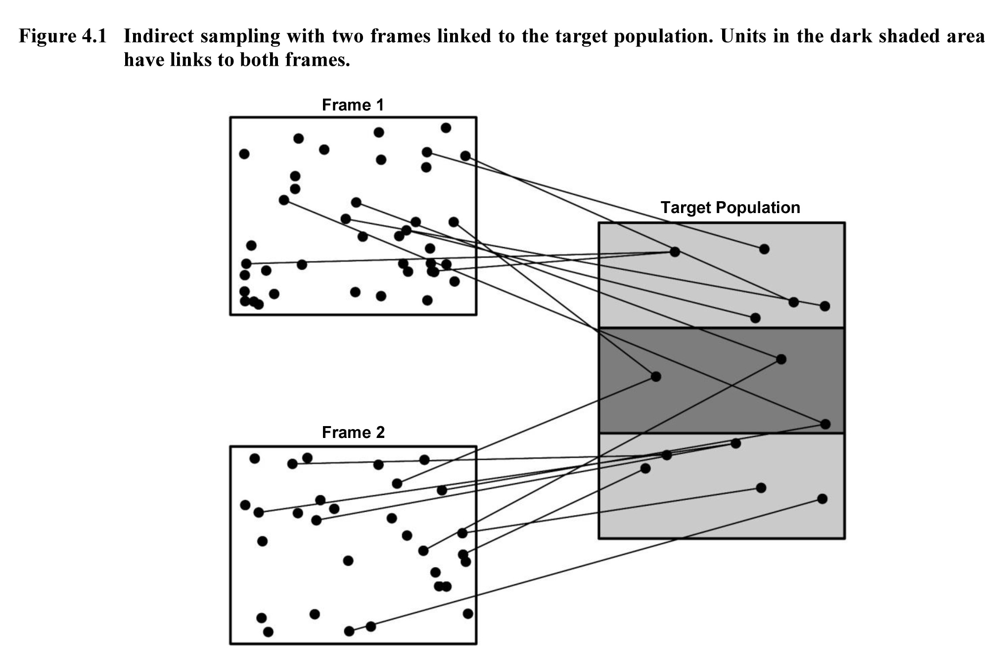
Figure 4.1 Indirect sampling with two frames linked to the target population. Units in the dark shaded area have links to both frames

Description for Figure 4.1

Figure illustrating an example of linkage structure. In the example, there is an indirect sampling with two frames (Frame 1 and Frame 2) linked to the target population. Units in the dark shaded area have links to both frames. A unit in the Target Population may have links to multiple units in Frame 1 and/or Frame 2. Furthermore, it is possible that the units of the Target Population can only be found in one of the two frames.

With indirect sampling, the Q MathType@MTEF@5@5@+= feaagKart1ev2aqatCvAUfeBSjuyZL2yd9gzLbvyNv2CaerbuLwBLn hiov2DGi1BTfMBaeXatLxBI9gBaerbd9wDYLwzYbItLDharqqtubsr 4rNCHbGeaGqiFu0Je9sqqrpepC0xbbL8F4rqqrFfpu0de9LqFHe9Lq pepeea0xd9q8as0=LqLs=Jirpepeea0=as0Fb9pgea0lrP0xe9Fve9 Fve9qapdbaqaaeGaciGaaiaabeqaamaabaabaaGcbaGaamyuaaaa@38EC@ frames can contain different types of units (the situation with different types of units was also considered by Hartley, 1974). We are not interested in overlap of the sampling frames (shown as nonoverlapping in Figure 4.1 because they contain different types of units) but in the overlap for the units in the target population. Sampled units in the target population have multiple chances of selection if they are linked to multiple units in one or both sampling frames.

Let l j , k ( q ) = 1 MathType@MTEF@5@5@+= feaagKart1ev2aqatCvAUfeBSjuyZL2yd9gzLbvyNv2CaerbuLwBLn hiov2DGi1BTfMBaeXatLxBI9gBaerbd9wDYLwzYbItLDharqqtubsr 4rNCHbGeaGqiFu0Je9sqqrpepC0xbbL8F4rqqrFfpu0de9LqFHe9Lq pepeea0xd9q8as0=LqLs=Jirpepeea0=as0Fb9pgea0lrP0xe9Fve9 Fve9qapdbaqaaeGaciGaaiaabeqaamaabaabaaGcbaGaamiBamaaDa aaleaacaWGQbGaaGilaiaaysW7caWGRbaabaGaaGikaiaadghacaaI PaaaaOGaaGjbVlaai2dacaaMe8UaaGymaaaa@4457@ if unit j MathType@MTEF@5@5@+= feaagKart1ev2aqatCvAUfeBSjuyZL2yd9gzLbvyNv2CaerbuLwBLn hiov2DGi1BTfMBaeXatLxBI9gBaerbd9wDYLwzYbItLDharqqtubsr 4rNCHbGeaGqiFu0Je9sqqrpepC0xbbL8F4rqqrFfpu0de9LqFHe9Lq pepeea0xd9q8as0=LqLs=Jirpepeea0=as0Fb9pgea0lrP0xe9Fve9 Fve9qapdbaqaaeGaciGaaiaabeqaamaabaabaaGcbaGaamOAaaaa@3905@ from Frame q MathType@MTEF@5@5@+= feaagKart1ev2aqatCvAUfeBSjuyZL2yd9gzLbvyNv2CaerbuLwBLn hiov2DGi1BTfMBaeXatLxBI9gBaerbd9wDYLwzYbItLDharqqtubsr 4rNCHbGeaGqiFu0Je9sqqrpepC0xbbL8F4rqqrFfpu0de9LqFHe9Lq pepeea0xd9q8as0=LqLs=Jirpepeea0=as0Fb9pgea0lrP0xe9Fve9 Fve9qapdbaqaaeGaciGaaiaabeqaamaabaabaaGcbaGaamyCaaaa@390C@ is linked to unit k MathType@MTEF@5@5@+= feaagKart1ev2aqatCvAUfeBSjuyZL2yd9gzLbvyNv2CaerbuLwBLn hiov2DGi1BTfMBaeXatLxBI9gBaerbd9wDYLwzYbItLDharqqtubsr 4rNCHbGeaGqiFu0Je9sqqrpepC0xbbL8F4rqqrFfpu0de9LqFHe9Lq pepeea0xd9q8as0=LqLs=Jirpepeea0=as0Fb9pgea0lrP0xe9Fve9 Fve9qapdbaqaaeGaciGaaiaabeqaamaabaabaaGcbaGaam4Aaaaa@3906@ in the target population, and let L k ( q ) MathType@MTEF@5@5@+= feaagKart1ev2aqatCvAUfeBSjuyZL2yd9gzLbvyNv2CaerbuLwBLn hiov2DGi1BTfMBaeXatLxBI9gBaerbd9wDYLwzYbItLDharqqtubsr 4rNCHbGeaGqiFu0Je9sqqrpepC0xbbL8F4rqqrFfpu0de9LqFHe9Lq pepeea0xd9q8as0=LqLs=Jirpepeea0=as0Fb9pgea0lrP0xe9Fve9 Fve9qapdbaqaaeGaciGaaiaabeqaamaabaabaaGcbaGaamitamaaDa aaleaacaWGRbaabaGaaGikaiaadghacaaIPaaaaaaa@3C5F@ be the total number of links between unit k MathType@MTEF@5@5@+= feaagKart1ev2aqatCvAUfeBSjuyZL2yd9gzLbvyNv2CaerbuLwBLn hiov2DGi1BTfMBaeXatLxBI9gBaerbd9wDYLwzYbItLDharqqtubsr 4rNCHbGeaGqiFu0Je9sqqrpepC0xbbL8F4rqqrFfpu0de9LqFHe9Lq pepeea0xd9q8as0=LqLs=Jirpepeea0=as0Fb9pgea0lrP0xe9Fve9 Fve9qapdbaqaaeGaciGaaiaabeqaamaabaabaaGcbaGaam4Aaaaa@3906@ in the target population and Frame q MathType@MTEF@5@5@+= feaagKart1ev2aqatCvAUfeBSjuyZL2yd9gzLbvyNv2CaerbuLwBLn hiov2DGi1BTfMBaeXatLxBI9gBaerbd9wDYLwzYbItLDharqqtubsr 4rNCHbGeaGqiFu0Je9sqqrpepC0xbbL8F4rqqrFfpu0de9LqFHe9Lq pepeea0xd9q8as0=LqLs=Jirpepeea0=as0Fb9pgea0lrP0xe9Fve9 Fve9qapdbaqaaeGaciGaaiaabeqaamaabaabaaGcbaGaamyCaaaa@390C@ (assumed to be knowable from asking unit k ) . MathType@MTEF@5@5@+= feaagKart1ev2aqatCvAUfeBSjuyZL2yd9gzLbvyNv2CaerbuLwBLn hiov2DGi1BTfMBaeXatLxBI9gBaerbd9wDYLwzYbItLDharqqtubsr 4rNCHbGeaGqiFu0Je9sqqrpepC0xbbL8F4rqqrFfpu0de9LqFHe9Lq pepeea0xd9q8as0=LqLs=Jirpepeea0=as0Fb9pgea0lrP0xe9Fve9 Fve9qapdbaqaaeGaciGaaiaabeqaamaabaabaaGcbaGaam4AaiaacM cacaGGUaaaaa@3A65@ Then an estimator Y ^ ( q ) MathType@MTEF@5@5@+= feaagKart1ev2aqatCvAUfeBSjuyZL2yd9gzLbvyNv2CaerbuLwBLn hiov2DGi1BTfMBaeXatLxBI9gBaerbd9wDYLwzYbItLDharqqtubsr 4rNCHbGeaGqiFu0Je9sqqrpepC0xbbL8F4rqqrFfpu0de9LqFHe9Lq pepeea0xd9q8as0=LqLs=Jirpepeea0=as0Fb9pgea0lrP0xe9Fve9 Fve9qapdbaqaaeGaciGaaiaabeqaamaabaabaaGcbaGabmywayaaja WaaWbaaSqabeaacaaIOaGaamyCaiaaiMcaaaaaaa@3B8C@ can be found for each frame using the links as

Y ^ ( q ) = j S ( q ) w j ( q ) k l j , k ( q ) L k ( q ) y k = k u k ( q ) y k , MathType@MTEF@5@5@+= feaagKart1ev2aaatCvAUfeBSjuyZL2yd9gzLbvyNv2CaerbuLwBLn hiov2DGi1BTfMBaeXatLxBI9gBaerbd9wDYLwzYbItLDharqqtubsr 4rNCHbGeaGqiFu0Je9sqqrpepC0xbbL8F4rqqrFfpu0de9LqFHe9Lq pepeea0xd9q8as0=LqLs=Jirpepeea0=as0Fb9pgea0lrP0xe9Fve9 Fve9qapdbaqaaeGaciGaaiaabeqaamaabaabaaGcbaGabmywayaaja WaaWbaaSqabeaacaaIOaGaamyCaiaaiMcaaaGccaaMe8UaaGypaiaa ysW7daaeqbqaaiaaykW7caWG3bWaa0baaSqaaiaadQgaaeaacaaIOa GaamyCaiaaiMcaaaGcdaaeqbqabSqaaiaadUgaaeqaniabggHiLdGc caaMe8+aaSaaaeaacaWGSbWaa0baaSqaaiaadQgacaaISaGaaGjbVl aadUgaaeaacaaIOaGaamyCaiaaiMcaaaaakeaacaWGmbWaa0baaSqa aiaadUgaaeaacaaIOaGaamyCaiaaiMcaaaaaaOGaaGjbVlaadMhada WgaaWcbaGaam4AaaqabaaabaGaamOAaiaaysW7cqGHiiIZcaaMe8Ua am4uamaaCaaameqabaGaaiikaiaadghacaGGPaaaaaWcbeqdcqGHri s5aOGaaGjbVlaai2dacaaMe8+aaabuaeaacaaMc8UaamyDamaaDaaa leaacaWGRbaabaGaaGikaiaadghacaaIPaaaaOGaamyEamaaBaaale aacaWGRbaabeaaaeaacaWGRbaabeqdcqGHris5aOGaaGilaaaa@74B1@

where

u k ( q ) = j S ( q ) w j ( q ) l j , k ( q ) L k ( q ) . MathType@MTEF@5@5@+= feaagKart1ev2aaatCvAUfeBSjuyZL2yd9gzLbvyNv2CaerbuLwBLn hiov2DGi1BTfMBaeXatLxBI9gBaerbd9wDYLwzYbItLDharqqtubsr 4rNCHbGeaGqiFu0Je9sqqrpepC0xbbL8F4rqqrFfpu0de9LqFHe9Lq pepeea0xd9q8as0=LqLs=Jirpepeea0=as0Fb9pgea0lrP0xe9Fve9 Fve9qapdbaqaaeGaciGaaiaabeqaamaabaabaaGcbaGaamyDamaaDa aaleaacaWGRbaabaGaaGikaiaadghacaaIPaaaaOGaaGjbVlaai2da caaMe8+aaabuaeaacaaMc8Uaam4DamaaDaaaleaacaWGQbaabaGaaG ikaiaadghacaaIPaaaaOGaaGjbVpaalaaabaGaamiBamaaDaaaleaa caWGQbGaaGilaiaaysW7caWGRbaabaGaaGikaiaadghacaaIPaaaaa GcbaGaamitamaaDaaaleaacaWGRbaabaGaaGikaiaadghacaaIPaaa aaaaaeaacaWGQbGaaGjbVlabgIGiolaaysW7caWGtbWaaWbaaWqabe aacaGGOaGaamyCaiaacMcaaaaaleqaniabggHiLdGccaaIUaaaaa@5FCC@

In the context of our example, person j MathType@MTEF@5@5@+= feaagKart1ev2aqatCvAUfeBSjuyZL2yd9gzLbvyNv2CaerbuLwBLn hiov2DGi1BTfMBaeXatLxBI9gBaerbd9wDYLwzYbItLDharqqtubsr 4rNCHbGeaGqiFu0Je9sqqrpepC0xbbL8F4rqqrFfpu0de9LqFHe9Lq pepeea0xd9q8as0=LqLs=Jirpepeea0=as0Fb9pgea0lrP0xe9Fve9 Fve9qapdbaqaaeGaciGaaiaabeqaamaabaabaaGcbaGaamOAaaaa@3905@ in S 1 MathType@MTEF@5@5@+= feaagKart1ev2aqatCvAUfeBSjuyZL2yd9gzLbvyNv2CaerbuLwBLn hiov2DGi1BTfMBaeXatLxBI9gBaerbd9wDYLwzYbItLDharqqtubsr 4rNCHbGeaGqiFu0Je9sqqrpepC0xbbL8F4rqqrFfpu0de9LqFHe9Lq pepeea0xd9q8as0=LqLs=Jirpepeea0=as0Fb9pgea0lrP0xe9Fve9 Fve9qapdbaqaaeGaciGaaiaabeqaamaabaabaaGcbaGaam4uamaaBa aaleaacaaIXaaabeaaaaa@39D5@ would say they receive paid home care from provider k , MathType@MTEF@5@5@+= feaagKart1ev2aqatCvAUfeBSjuyZL2yd9gzLbvyNv2CaerbuLwBLn hiov2DGi1BTfMBaeXatLxBI9gBaerbd9wDYLwzYbItLDharqqtubsr 4rNCHbGeaGqiFu0Je9sqqrpepC0xbbL8F4rqqrFfpu0de9LqFHe9Lq pepeea0xd9q8as0=LqLs=Jirpepeea0=as0Fb9pgea0lrP0xe9Fve9 Fve9qapdbaqaaeGaciGaaiaabeqaamaabaabaaGcbaGaam4AaiaacY caaaa@39B6@ resulting in l j , k ( 1 ) = 1. MathType@MTEF@5@5@+= feaagKart1ev2aqatCvAUfeBSjuyZL2yd9gzLbvyNv2CaerbuLwBLn hiov2DGi1BTfMBaeXatLxBI9gBaerbd9wDYLwzYbItLDharqqtubsr 4rNCHbGeaGqiFu0Je9sqqrpepC0xbbL8F4rqqrFfpu0de9LqFHe9Lq pepeea0xd9q8as0=LqLs=Jirpepeea0=as0Fb9pgea0lrP0xe9Fve9 Fve9qapdbaqaaeGaciGaaiaabeqaamaabaabaaGcbaGaamiBamaaDa aaleaacaWGQbGaaGilaiaaysW7caWGRbaabaGaaGikaiaaigdacaaI PaaaaOGaaGjbVlaai2dacaaMe8UaaGymaiaac6caaaa@44CE@ Then the linked home care provider would be asked about how many other persons they work for who receive Medicare (assume they would know this or it could be determined from other sources), giving the value L k ( 1 ) . MathType@MTEF@5@5@+= feaagKart1ev2aqatCvAUfeBSjuyZL2yd9gzLbvyNv2CaerbuLwBLn hiov2DGi1BTfMBaeXatLxBI9gBaerbd9wDYLwzYbItLDharqqtubsr 4rNCHbGeaGqiFu0Je9sqqrpepC0xbbL8F4rqqrFfpu0de9LqFHe9Lq pepeea0xd9q8as0=LqLs=Jirpepeea0=as0Fb9pgea0lrP0xe9Fve9 Fve9qapdbaqaaeGaciGaaiaabeqaamaabaabaaGcbaGaamitamaaDa aaleaacaWGRbaabaGaaGikaiaaigdacaaIPaaaaOGaaiOlaaaa@3CE0@ The quantity u k ( q ) MathType@MTEF@5@5@+= feaagKart1ev2aqatCvAUfeBSjuyZL2yd9gzLbvyNv2CaerbuLwBLn hiov2DGi1BTfMBaeXatLxBI9gBaerbd9wDYLwzYbItLDharqqtubsr 4rNCHbGeaGqiFu0Je9sqqrpepC0xbbL8F4rqqrFfpu0de9LqFHe9Lq pepeea0xd9q8as0=LqLs=Jirpepeea0=as0Fb9pgea0lrP0xe9Fve9 Fve9qapdbaqaaeGaciGaaiaabeqaamaabaabaaGcbaGaamyDamaaDa aaleaacaWGRbaabaGaaGikaiaadghacaaIPaaaaaaa@3C88@ sums the weights of the units in S q MathType@MTEF@5@5@+= feaagKart1ev2aqatCvAUfeBSjuyZL2yd9gzLbvyNv2CaerbuLwBLn hiov2DGi1BTfMBaeXatLxBI9gBaerbd9wDYLwzYbItLDharqqtubsr 4rNCHbGeaGqiFu0Je9sqqrpepC0xbbL8F4rqqrFfpu0de9LqFHe9Lq pepeea0xd9q8as0=LqLs=Jirpepeea0=as0Fb9pgea0lrP0xe9Fve9 Fve9qapdbaqaaeGaciGaaiaabeqaamaabaabaaGcbaGaam4uamaaBa aaleaacaWGXbaabeaaaaa@3A10@ with links to unit k , MathType@MTEF@5@5@+= feaagKart1ev2aqatCvAUfeBSjuyZL2yd9gzLbvyNv2CaerbuLwBLn hiov2DGi1BTfMBaeXatLxBI9gBaerbd9wDYLwzYbItLDharqqtubsr 4rNCHbGeaGqiFu0Je9sqqrpepC0xbbL8F4rqqrFfpu0de9LqFHe9Lq pepeea0xd9q8as0=LqLs=Jirpepeea0=as0Fb9pgea0lrP0xe9Fve9 Fve9qapdbaqaaeGaciGaaiaabeqaamaabaabaaGcbaGaam4AaiaacY caaaa@39B6@ adjusting for the multiplicity of the links to that frame. If w j ( q ) = 1 / π j ( q ) , MathType@MTEF@5@5@+= feaagKart1ev2aqatCvAUfeBSjuyZL2yd9gzLbvyNv2CaerbuLwBLn hiov2DGi1BTfMBaeXatLxBI9gBaerbd9wDYLwzYbItLDharqqtubsr 4rNCHbGeaGqiFu0Je9sqqrpepC0xbbL8F4rqqrFfpu0de9LqFHe9Lq pepeea0xd9q8as0=LqLs=Jirpepeea0=as0Fb9pgea0lrP0xe9Fve9 Fve9qapdbaqaaeGaciGaaiaabeqaamaabaabaaGcbaGaam4DamaaDa aaleaacaWGQbaabaGaaGikaiaadghacaaIPaaaaOGaaGjbVlaai2da caaMe8+aaSGbaeaacaaIXaGaaGPaVdqaaiabec8aWnaaDaaaleaaca WGQbaabaGaaGikaiaadghacaaIPaaaaaaakiaacYcaaaa@48BE@ then

E [ u k ( q ) ] = E [ j S ( q ) w j ( q ) l j , k ( q ) L k ( q ) ] = a k ( q ) , MathType@MTEF@5@5@+= feaagKart1ev2aaatCvAUfeBSjuyZL2yd9gzLbvyNv2CaerbuLwBLn hiov2DGi1BTfMBaeXatLxBI9gBaerbd9wDYLwzYbItLDharqqtubsr 4rNCHbGeaGqiFu0Je9sqqrpepC0xbbL8F4rqqrFfpu0de9LqFHe9Lq pepeea0xd9q8as0=LqLs=Jirpepeea0=as0Fb9pgea0lrP0xe9Fve9 Fve9qapdbaqaaeGaciGaaiaabeqaamaabaabaaGcbaGaamyraiaayk W7caaIBbGaamyDamaaDaaaleaacaWGRbaabaGaaGikaiaadghacaaI PaaaaOGaaGyxaiaaysW7caaI9aGaaGjbVlaadweadaWadaqaamaaqa fabaGaaGPaVlaadEhadaqhaaWcbaGaamOAaaqaaiaaiIcacaWGXbGa aGykaaaakmaalaaabaGaamiBamaaDaaaleaacaWGQbGaaGilaiaays W7caWGRbaabaGaaGikaiaadghacaaIPaaaaaGcbaGaamitamaaDaaa leaacaWGRbaabaGaaGikaiaadghacaaIPaaaaaaaaeaacaWGQbGaaG jbVlabgIGiolaaysW7caWGtbWaaWbaaWqabeaacaGGOaGaamyCaiaa cMcaaaaaleqaniabggHiLdaakiaawUfacaGLDbaacaaMe8UaaGypai aaysW7caWGHbWaa0baaSqaaiaadUgaaeaacaaIOaGaamyCaiaaiMca aaGccaaISaaaaa@6D63@

where a k ( q ) = 1 MathType@MTEF@5@5@+= feaagKart1ev2aqatCvAUfeBSjuyZL2yd9gzLbvyNv2CaerbuLwBLn hiov2DGi1BTfMBaeXatLxBI9gBaerbd9wDYLwzYbItLDharqqtubsr 4rNCHbGeaGqiFu0Je9sqqrpepC0xbbL8F4rqqrFfpu0de9LqFHe9Lq pepeea0xd9q8as0=LqLs=Jirpepeea0=as0Fb9pgea0lrP0xe9Fve9 Fve9qapdbaqaaeGaciGaaiaabeqaamaabaabaaGcbaGaamyyamaaDa aaleaacaWGRbaabaGaaGikaiaadghacaaIPaaaaOGaaGjbVlaai2da caaMe8UaaGymaaaa@411A@ if target population member k MathType@MTEF@5@5@+= feaagKart1ev2aqatCvAUfeBSjuyZL2yd9gzLbvyNv2CaerbuLwBLn hiov2DGi1BTfMBaeXatLxBI9gBaerbd9wDYLwzYbItLDharqqtubsr 4rNCHbGeaGqiFu0Je9sqqrpepC0xbbL8F4rqqrFfpu0de9LqFHe9Lq pepeea0xd9q8as0=LqLs=Jirpepeea0=as0Fb9pgea0lrP0xe9Fve9 Fve9qapdbaqaaeGaciGaaiaabeqaamaabaabaaGcbaGaam4Aaaaa@3906@ is linked to at least one unit in Frame q MathType@MTEF@5@5@+= feaagKart1ev2aqatCvAUfeBSjuyZL2yd9gzLbvyNv2CaerbuLwBLn hiov2DGi1BTfMBaeXatLxBI9gBaerbd9wDYLwzYbItLDharqqtubsr 4rNCHbGeaGqiFu0Je9sqqrpepC0xbbL8F4rqqrFfpu0de9LqFHe9Lq pepeea0xd9q8as0=LqLs=Jirpepeea0=as0Fb9pgea0lrP0xe9Fve9 Fve9qapdbaqaaeGaciGaaiaabeqaamaabaabaaGcbaGaamyCaaaa@390C@ and 0 otherwise.

Multiple-frame methods may then be used to estimate characteristics of the population of home care providers, assuming that unit k MathType@MTEF@5@5@+= feaagKart1ev2aqatCvAUfeBSjuyZL2yd9gzLbvyNv2CaerbuLwBLn hiov2DGi1BTfMBaeXatLxBI9gBaerbd9wDYLwzYbItLDharqqtubsr 4rNCHbGeaGqiFu0Je9sqqrpepC0xbbL8F4rqqrFfpu0de9LqFHe9Lq pepeea0xd9q8as0=LqLs=Jirpepeea0=as0Fb9pgea0lrP0xe9Fve9 Fve9qapdbaqaaeGaciGaaiaabeqaamaabaabaaGcbaGaam4Aaaaa@3906@ linked from S q MathType@MTEF@5@5@+= feaagKart1ev2aqatCvAUfeBSjuyZL2yd9gzLbvyNv2CaerbuLwBLn hiov2DGi1BTfMBaeXatLxBI9gBaerbd9wDYLwzYbItLDharqqtubsr 4rNCHbGeaGqiFu0Je9sqqrpepC0xbbL8F4rqqrFfpu0de9LqFHe9Lq pepeea0xd9q8as0=LqLs=Jirpepeea0=as0Fb9pgea0lrP0xe9Fve9 Fve9qapdbaqaaeGaciGaaiaabeqaamaabaabaaGcbaGaam4uamaaBa aaleaacaWGXbaabeaaaaa@3A10@ provides accurate information on (1) the number of links to members of Frame q ( L k ( q ) ) , MathType@MTEF@5@5@+= feaagKart1ev2aqatCvAUfeBSjuyZL2yd9gzLbvyNv2CaerbuLwBLn hiov2DGi1BTfMBaeXatLxBI9gBaerbd9wDYLwzYbItLDharqqtubsr 4rNCHbGeaGqiFu0Je9sqqrpepC0xbbL8F4rqqrFfpu0de9LqFHe9Lq pepeea0xd9q8as0=LqLs=Jirpepeea0=as0Fb9pgea0lrP0xe9Fve9 Fve9qapdbaqaaeGaciGaaiaabeqaamaabaabaaGcbaGaamyCaiaays W7caaIOaGaamitamaaDaaaleaacaWGRbaabaGaaGikaiaadghacaaI PaaaaOGaaGykaiaacYcaaaa@4101@ needed for multiplicity adjustments with Frame q , MathType@MTEF@5@5@+= feaagKart1ev2aqatCvAUfeBSjuyZL2yd9gzLbvyNv2CaerbuLwBLn hiov2DGi1BTfMBaeXatLxBI9gBaerbd9wDYLwzYbItLDharqqtubsr 4rNCHbGeaGqiFu0Je9sqqrpepC0xbbL8F4rqqrFfpu0de9LqFHe9Lq pepeea0xd9q8as0=LqLs=Jirpepeea0=as0Fb9pgea0lrP0xe9Fve9 Fve9qapdbaqaaeGaciGaaiaabeqaamaabaabaaGcbaGaamyCaiaacY caaaa@39BC@ and (2) whether they are also linked to the other frame(s) ( a k ( f ) MathType@MTEF@5@5@+= feaagKart1ev2aqatCvAUfeBSjuyZL2yd9gzLbvyNv2CaerbuLwBLn hiov2DGi1BTfMBaeXatLxBI9gBaerbd9wDYLwzYbItLDharqqtubsr 4rNCHbGeaGqiFu0Je9sqqrpepC0xbbL8F4rqqrFfpu0de9LqFHe9Lq pepeea0xd9q8as0=LqLs=Jirpepeea0=as0Fb9pgea0lrP0xe9Fve9 Fve9qapdbaqaaeGaciGaaiaabeqaamaabaabaaGcbaGaaiikaiaadg gadaqhaaWcbaGaam4AaaqaaiaaiIcacaWGMbGaaGykaaaaaaa@3D15@ for f q ) , MathType@MTEF@5@5@+= feaagKart1ev2aqatCvAUfeBSjuyZL2yd9gzLbvyNv2CaerbuLwBLn hiov2DGi1BTfMBaeXatLxBI9gBaerbd9wDYLwzYbItLDharqqtubsr 4rNCHbGeaGqiFu0Je9sqqrpepC0xbbL8F4rqqrFfpu0de9LqFHe9Lq pepeea0xd9q8as0=LqLs=Jirpepeea0=as0Fb9pgea0lrP0xe9Fve9 Fve9qapdbaqaaeGaciGaaiaabeqaamaabaabaaGcbaGaamOzaiaays W7cqGHGjsUcaaMe8UaamyCaiaacMcacaGGSaaaaa@4035@ needed to adjust for the multiplicity of linkage from different frames.

Lavallée and Rivest (2012) noted that if the union of the two frames has incomplete coverage  MathType@MTEF@5@5@+= feaagKart1ev2aqatCvAUfeBSjuyZL2yd9gzLbvyNv2CaerbuLwBLn hiov2DGi1BTfMBaeXatLxBI9gBaerbd9wDYLwzYbItLDharqqtubsr 4rNCHbGeaGqiVu0Je9sqqrpepC0xbbL8F4rqqrFfpeea0xe9Lq=Jc9 vqaqpepm0xbba9pwe9Q8fs0=yqaqpepae9pg0FirpepeKkFr0xfr=x fr=xb9adbaqaaeGaciGaaiaabeqaamaabaabaaGcbaacbaqcLbwaqa aaaaaaaaWdbiaa=nbiaaa@37A3@  Assumption (A1) is violated  MathType@MTEF@5@5@+= feaagKart1ev2aqatCvAUfeBSjuyZL2yd9gzLbvyNv2CaerbuLwBLn hiov2DGi1BTfMBaeXatLxBI9gBaerbd9wDYLwzYbItLDharqqtubsr 4rNCHbGeaGqiVu0Je9sqqrpepC0xbbL8F4rqqrFfpeea0xe9Lq=Jc9 vqaqpepm0xbba9pwe9Q8fs0=yqaqpepae9pg0FirpepeKkFr0xfr=x fr=xb9adbaqaaeGaciGaaiaabeqaamaabaabaaGcbaacbaqcLbwaqa aaaaaaaaWdbiaa=nbiaaa@37A3@  the samples from the two frames can be used to estimate the size of the target population. Let T ^ ( q ) = k u k ( q ) MathType@MTEF@5@5@+= feaagKart1ev2aqatCvAUfeBSjuyZL2yd9gzLbvyNv2CaerbuLwBLn hiov2DGi1BTfMBaeXatLxBI9gBaerbd9wDYLwzYbItLDharqqtubsr 4rNCHbGeaGqiFu0Je9sqqrpepC0xbbL8F4rqqrFfpu0de9LqFHe9Lq pepeea0xd9q8as0=LqLs=Jirpepeea0=as0Fb9pgea0lrP0xe9Fve9 Fve9qapdbaqaaeGaciGaaiaabeqaamaabaabaaGcbaGabmivayaaja WaaWbaaSqabeaacaaIOaGaamyCaiaaiMcaaaGccaaMe8UaaGypaiaa ysW7daaeqaqaaiaaykW7caWG1bWaa0baaSqaaiaadUgaaeaacaaIOa GaamyCaiaaiMcaaaaabaGaam4Aaaqab0GaeyyeIuoaaaa@4837@ for k = 1, 2. MathType@MTEF@5@5@+= feaagKart1ev2aqatCvAUfeBSjuyZL2yd9gzLbvyNv2CaerbuLwBLn hiov2DGi1BTfMBaeXatLxBI9gBaerbd9wDYLwzYbItLDharqqtubsr 4rNCHbGeaGqiFu0Je9sqqrpepC0xbbL8F4rqqrFfpu0de9LqFHe9Lq pepeea0xd9q8as0=LqLs=Jirpepeea0=as0Fb9pgea0lrP0xe9Fve9 Fve9qapdbaqaaeGaciGaaiaabeqaamaabaabaaGcbaGaam4Aaiaays W7caaI9aGaaGjbVlaaigdacaaISaGaaGjbVlaaikdacaGGUaaaaa@4153@ Then E [ T ^ ( q ) ] MathType@MTEF@5@5@+= feaagKart1ev2aqatCvAUfeBSjuyZL2yd9gzLbvyNv2CaerbuLwBLn hiov2DGi1BTfMBaeXatLxBI9gBaerbd9wDYLwzYbItLDharqqtubsr 4rNCHbGeaGqiFu0Je9sqqrpepC0xbbL8F4rqqrFfpu0de9LqFHe9Lq pepeea0xd9q8as0=LqLs=Jirpepeea0=as0Fb9pgea0lrP0xe9Fve9 Fve9qapdbaqaaeGaciGaaiaabeqaamaabaabaaGcbaGaamyraiaayk W7daWadeqaaiqadsfagaqcamaaCaaaleqabaGaaGikaiaadghacaaI PaaaaaGccaGLBbGaayzxaaaaaa@3FD9@ is the number of target population members that can be linked from Frame q MathType@MTEF@5@5@+= feaagKart1ev2aqatCvAUfeBSjuyZL2yd9gzLbvyNv2CaerbuLwBLn hiov2DGi1BTfMBaeXatLxBI9gBaerbd9wDYLwzYbItLDharqqtubsr 4rNCHbGeaGqiFu0Je9sqqrpepC0xbbL8F4rqqrFfpu0de9LqFHe9Lq pepeea0xd9q8as0=LqLs=Jirpepeea0=as0Fb9pgea0lrP0xe9Fve9 Fve9qapdbaqaaeGaciGaaiaabeqaamaabaabaaGcbaGaamyCaaaa@390C@ . Each sample also provides an estimate of the number of target population units that can be linked from both frames: T ^ { 1, 2 } ( 1 ) = k u k ( 1 ) a k ( 2 ) MathType@MTEF@5@5@+= feaagKart1ev2aqatCvAUfeBSjuyZL2yd9gzLbvyNv2CaerbuLwBLn hiov2DGi1BTfMBaeXatLxBI9gBaerbd9wDYLwzYbItLDharqqtubsr 4rNCHbGeaGqiFu0Je9sqqrpepC0xbbL8F4rqqrFfpu0de9LqFHe9Lq pepeea0xd9q8as0=LqLs=Jirpepeea0=as0Fb9pgea0lrP0xe9Fve9 Fve9qapdbaqaaeGaciGaaiaabeqaamaabaabaaGcbaGabmivayaaja Waa0baaSqaaiaaiUhacaaIXaGaaGilaiaaysW7caaIYaGaaGyFaaqa aiaaiIcacaaIXaGaaGykaaaakiaaysW7caaI9aGaaGjbVpaaqababa GaaGPaVlaadwhadaqhaaWcbaGaam4AaaqaaiaaiIcacaaIXaGaaGyk aaaakiaadggadaqhaaWcbaGaam4AaaqaaiaaiIcacaaIYaGaaGykaa aaaeaacaWGRbaabeqdcqGHris5aaaa@51B5@ and T ^ { 1, 2 } ( 2 ) = k u k ( 2 ) a k ( 1 ) . MathType@MTEF@5@5@+= feaagKart1ev2aqatCvAUfeBSjuyZL2yd9gzLbvyNv2CaerbuLwBLn hiov2DGi1BTfMBaeXatLxBI9gBaerbd9wDYLwzYbItLDharqqtubsr 4rNCHbGeaGqiFu0Je9sqqrpepC0xbbL8F4rqqrFfpu0de9LqFHe9Lq pepeea0xd9q8as0=LqLs=Jirpepeea0=as0Fb9pgea0lrP0xe9Fve9 Fve9qapdbaqaaeGaciGaaiaabeqaamaabaabaaGcbaGabmivayaaja Waa0baaSqaaiaaiUhacaaIXaGaaGilaiaaysW7caaIYaGaaGyFaaqa aiaaiIcacaaIYaGaaGykaaaakiaaysW7caaI9aGaaGjbVpaaqababa GaaGPaVlaadwhadaqhaaWcbaGaam4AaaqaaiaaiIcacaaIYaGaaGyk aaaakiaadggadaqhaaWcbaGaam4AaaqaaiaaiIcacaaIXaGaaGykaa aaaeaacaWGRbaabeqdcqGHris5aOGaaiOlaaaa@5272@ These can be composited to obtain an estimator T ^ { 1, 2 } MathType@MTEF@5@5@+= feaagKart1ev2aqatCvAUfeBSjuyZL2yd9gzLbvyNv2CaerbuLwBLn hiov2DGi1BTfMBaeXatLxBI9gBaerbd9wDYLwzYbItLDharqqtubsr 4rNCHbGeaGqiFu0Je9sqqrpepC0xbbL8F4rqqrFfpu0de9LqFHe9Lq pepeea0xd9q8as0=LqLs=Jirpepeea0=as0Fb9pgea0lrP0xe9Fve9 Fve9qapdbaqaaeGaciGaaiaabeqaamaabaabaaGcbaGabmivayaaja WaaSbaaSqaaiaaiUhacaaIXaGaaGilaiaaysW7caaIYaGaaGyFaaqa baaaaa@3EF1@ of the number of persons in the target population who can be captured from both frames.

The Lincoln-Petersen capture-recapture estimator of population size can then be used. Under the strong assumption that being captured by Frame 1 is independent of being captured by Frame 2, the total number of home care providers can be estimated by T ^ ( 1 ) T ^ ( 2 ) / T ^ { 1, 2 } . MathType@MTEF@5@5@+= feaagKart1ev2aqatCvAUfeBSjuyZL2yd9gzLbvyNv2CaerbuLwBLn hiov2DGi1BTfMBaeXatLxBI9gBaerbd9wDYLwzYbItLDharqqtubsr 4rNCHbGeaGqiFu0Je9sqqrpepC0xbbL8F4rqqrFfpu0de9LqFHe9Lq pepeea0xd9q8as0=LqLs=Jirpepeea0=as0Fb9pgea0lrP0xe9Fve9 Fve9qapdbaqaaeGaciGaaiaabeqaamaabaabaaGcbaWaaSGbaeaace WGubGbaKaadaahaaWcbeqaaiaaiIcacaaIXaGaaGykaaaakiqadsfa gaqcamaaCaaaleqabaGaaGikaiaaikdacaaIPaaaaaGcbaGabmivay aajaWaaSbaaSqaaiaaiUhacaaIXaGaaGilaiaaysW7caaIYaGaaGyF aaqabaaaaOGaaiOlaaaa@4644@ In some cases where the independence assumption is not met for the entire population, it may be approximately met on subpopulations whose estimated numbers can be summed. If there are more than two frames, loglinear models may be used to explore associations among the frames (Lohr, 2022, Chapter 14); Zhang (2019) presented a model for the situation in which frames may contain misclassified units.

Alleva, Arbia, Falorsi, Nardelli and Zuliani (2020) proposed using indirect multiple-frame sampling to estimate the number of people infected by SARS-CoV-2 during the early stages of the COVID-19 pandemic in 2020  MathType@MTEF@5@5@+= feaagKart1ev2aqatCvAUfeBSjuyZL2yd9gzLbvyNv2CaerbuLwBLn hiov2DGi1BTfMBaeXatLxBI9gBaerbd9wDYLwzYbItLDharqqtubsr 4rNCHbGeaGqiVu0Je9sqqrpepC0xbbL8F4rqqrFfpeea0xe9Lq=Jc9 vqaqpepm0xbba9pwe9Q8fs0=yqaqpepae9pg0FirpepeKkFr0xfr=x fr=xb9adbaqaaeGaciGaaiaabeqaamaabaabaaGcbaacbaqcLbwaqa aaaaaaaaWdbiaa=nbiaaa@37A3@  information needed for estimating transmissibility and infection parameters in epidemiologic models. In this application, Frame 1 consists of persons with verified infections (perhaps obtained from hospitals, quarantine centers, or clinics), and Frame 2 consists of other persons; the persons in S 2 MathType@MTEF@5@5@+= feaagKart1ev2aqatCvAUfeBSjuyZL2yd9gzLbvyNv2CaerbuLwBLn hiov2DGi1BTfMBaeXatLxBI9gBaerbd9wDYLwzYbItLDharqqtubsr 4rNCHbGeaGqiFu0Je9sqqrpepC0xbbL8F4rqqrFfpu0de9LqFHe9Lq pepeea0xd9q8as0=LqLs=Jirpepeea0=as0Fb9pgea0lrP0xe9Fve9 Fve9qapdbaqaaeGaciGaaiaabeqaamaabaabaaGcbaGaam4uamaaBa aaleaacaaIYaaabeaaaaa@39D6@ are administered a test for SARS-CoV-2. The linked sample consists of persons who had contact within the past 14 days with anyone in S 1 MathType@MTEF@5@5@+= feaagKart1ev2aqatCvAUfeBSjuyZL2yd9gzLbvyNv2CaerbuLwBLn hiov2DGi1BTfMBaeXatLxBI9gBaerbd9wDYLwzYbItLDharqqtubsr 4rNCHbGeaGqiFu0Je9sqqrpepC0xbbL8F4rqqrFfpu0de9LqFHe9Lq pepeea0xd9q8as0=LqLs=Jirpepeea0=as0Fb9pgea0lrP0xe9Fve9 Fve9qapdbaqaaeGaciGaaiaabeqaamaabaabaaGcbaGaam4uamaaBa aaleaacaaIXaaabeaaaaa@39D5@ or with a member of S 2 MathType@MTEF@5@5@+= feaagKart1ev2aqatCvAUfeBSjuyZL2yd9gzLbvyNv2CaerbuLwBLn hiov2DGi1BTfMBaeXatLxBI9gBaerbd9wDYLwzYbItLDharqqtubsr 4rNCHbGeaGqiFu0Je9sqqrpepC0xbbL8F4rqqrFfpu0de9LqFHe9Lq pepeea0xd9q8as0=LqLs=Jirpepeea0=as0Fb9pgea0lrP0xe9Fve9 Fve9qapdbaqaaeGaciGaaiaabeqaamaabaabaaGcbaGaam4uamaaBa aaleaacaaIYaaabeaaaaa@39D6@ who tested positive.


Date modified: