With-replacement bootstrap variance estimation for household surveys Principles, examples and implementation
Section 2. Notation and estimation
In this section, we define our main notations, and we
describe the sampling and estimation process. We first consider in Section 2.1
the case when a sample of households only is selected, and we describe the
estimation process which includes treatment of unit non-response and
calibration. We indicate in each case what is the benchmark variance estimator
considered, i.e. the variance estimator that we aim at reproducing for the
estimation of a total with the bootstrap method proposed in Section 3. The
case when individuals are sub-sampled inside households is covered in Section 2.2.
The benchmark variance estimators for this second case are given in Appendix A.
2.1 Case of a sample of households only
We consider estimation for a population
of households. We let
denote the value taken by some variable of
interest for the household
We are interested in the estimation of the
total
2.1.1 Sampling design
We suppose that a sample
is selected in
by means of a stratified one-stage sampling
design. The population
is partitioned into
strata
the samples
are selected inside independently, and the
sample
is the union of these samples. We let
denote the inclusion probability of a given
household
The design weight is
In case of full response, the estimator of
is
We consider as a benchmark variance estimator
with
the size of the sample
This variance estimator is unbiased if the samples are
selected inside strata by multinomial sampling (Tillé, 2011, Section 5.4),
a.k.a. sampling with replacement. It is conservative if the sampling designs
used inside strata are more efficient than multinomial sampling (Särndal, Swensson
and Wretman, 1992, Section 4.6), which we assume to hold true in the rest of the paper. The
positive bias of this variance estimator is expected to be negligible when the
sampling rates inside strata are themselves negligible, which is often the case
in phone surveys. This is illustrated by the results of our simulation study,
see Section 4.
2.1.2 Treatment of non-response
In practice, the sample
is prone to unit non-response, which leads to
the observation of a sub-sample of respondents
only. We let
denote the response indicator of a household
and
denote the response probability of the
household
We suppose that the households respond
independently of one another. Also, we suppose that unit non-response is
handled through the method of Response Homogeneity Groups (RHGs), which is
popular in practice (e.g. Brick, 2013;
Juillard and Chauvet, 2018). Under this framework, it is assumed that
the sample
may be partitioned into
RHGs denoted as
such that the response probability
is constant inside a RHG.
For
we let
denote the common response probability inside
the RHG
It is estimated by
with
some weight attached to the household
The choice
leads to estimating
by the unweighted response rate inside the
RHG. The choice
leads to estimating
by the response rate inside the RHG, weighted
by the sampling weights (e.g. Kott, 2012).
Accounting for the estimated response probabilities
leads to the weights corrected for non-response
with
the RHG of the household
The estimator of
adjusted for non-response is
Building on the multinomial variance estimator in (2.4)
and on linearization for estimators reweighted for unit-non-response (Kim and Kim, 2007, Section 2),
our benchmark variance estimator is
with
and
This is a conservative estimator for the asymptotic variance of
A key assumption for this to hold is that the
response indicators
are mutually independent.
2.1.3 Calibration
Lastly, the weights adjusted for non-response are
calibrated on auxiliary totals known on the population. For simplicity, we
describe only the Generalized REGression estimator (GREG, Särndal et al.,
1992, Chapter 6). Let
denote the vector of calibration variables at
the household level, and
the total on the population
For the sample
this leads to the linear calibrated weights
with
and where
is the estimator of
obtained by plugging
into (2.7). The calibrated estimator is
The sampling and estimation steps are summarized in Figure 2.1.
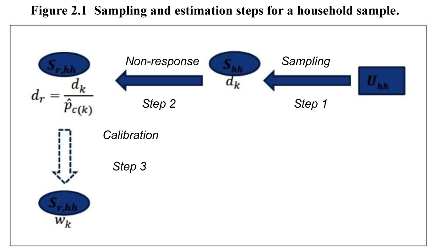
Description for Figure 2.1
Figure summarizing Sections 2.1.1
to 2.1.3, i.e., sampling and estimation steps for a household sample. The first
step consists in randomly selecting a sample, denoted
from a population, denoted
by means of a stratified one-stage sampling
design. Each unit of this sample has a survey weights, denoted
The second step consists in the treatment of
the non-response in the selected sample. The survey weights are adjusted to
take into account the non-response, now, denoted
In the third and final step, the weights
adjusted for non-response are calibrated on auxiliary totals known on the
population, finally denoted
Using linearization for estimators reweighted for
unit-non-response and calibrated (Kim
and Kim, 2007, Section 5), our benchmark variance estimator is
with
and
where we let
with
denote the estimated regression residuals of the variable of interest on
the calibration variables. This is a conservative estimator for the asymptotic
variance of
2.1.4 Computation of household weights on an example
To fix ideas, we describe a small example. We consider a
population
of
households. We suppose without loss of
generality that a single stratum is used, and that a sample of
households is selected.
The sample is
The inclusion probabilities of the selected
units are (say)
and
resulting in the design weights
and
Among the 10 selected households, 7 only are surveyed
due to non-response. It is accounted for by using the method of RHGs, with two
groups: the units
and
in the first one, and the units
and
in the second one. The units
and
are non-respondents. Inside each RHG, we
compute estimated response probabilities, weighted by the design weights
This leads to
The weights accounting for non-response are obtained for the respondents
by dividing the sampling weights by the estimated response probabilities. This
leads to the weights
Finally, the weights are calibrated to match exactly the population size
and an auxiliary total
Note that, using the sample of respondents, we obtain
and
66.53. The calibrated weights are
The sampling and estimation steps are summarized in Figure 2.2.

Description for Figure 2.2
Figure summarizing Section 2.1.4,
i.e., computation of household weights with an example. The figure illustrates
with an example the steps explained in Sections 2.1.1 to 2.1.3. In this
example, households B, C and G are non-respondents.
2.2 Case of a sample of households and individuals
We are interested in the population
of individuals associated to the population
of households considered in Section 2.1.
If we let
denote the value taken by some variable of
interest for the individual
the parameter of interest is
2.2.1 Sampling design
Within any sampled household
a subsample
of individuals is selected, and the sample
is the union of these samples. We let
denote the conditional inclusion probability
of the individual
inside the household
The conditional design weight of
is
for any
and the non-conditional design weight is
for any
In case of full response, the estimator of
is
The benchmark variance estimator for
is obtained from (2.4), by replacing
with
2.2.2 Treatment of non-response
The weights of individuals accounting for the
non-response of households are
with
the household containing
with
the weight of household
corrected for unit non-response (see equation (2.6)),
and
the conditional sampling weight of individual
inside the household
(see equation (2.19)). We let
denote the set of all sampled individuals inside the responding
households.
The individuals in
are themselves prone to non-response, though
it is usually expected to be to a smaller extent. This leads to the observation
of a sub-sample of respondents
only. We let
denote the response indicator and
denote the response probability of the
individual
.
We suppose that the individuals respond independently of one another. Also, we
suppose that this non-response is handled through the method of RHGs: the
sample
may be partitioned into
RHGs denoted as
such that the response probability
is constant inside a RHG.
For
we let
denote the common response probability inside
the RHG
It is estimated by
with
some weight attached to the individual
The choice
leads to estimating
by the unweighted response rate inside the
RHG. The choice
leads to estimating
by the response rate inside the RHG, weighted
by the individual sampling weights. The choice
leads to estimating
by the response rate inside the RHG, weighted
by the individual sampling weights corrected of household unit non-response. We
compare these different choices in the simulation study performed in Section 4.
Accounting for the estimated response probabilities
leads to the individual weights corrected for household/individual non-response
with
the household containing
The estimator of
adjusted for household/individual non-response
is
2.2.3 Calibration
We let
denote the vector of calibration variables at
the individual level, and
denote the total on the population
For the sample
this leads to the linear calibrated weights
with
and where
is the estimator of
obtained by plugging
into (2.27). The calibrated estimator is
The sampling and estimation steps are summarized in
Figure 2.3.
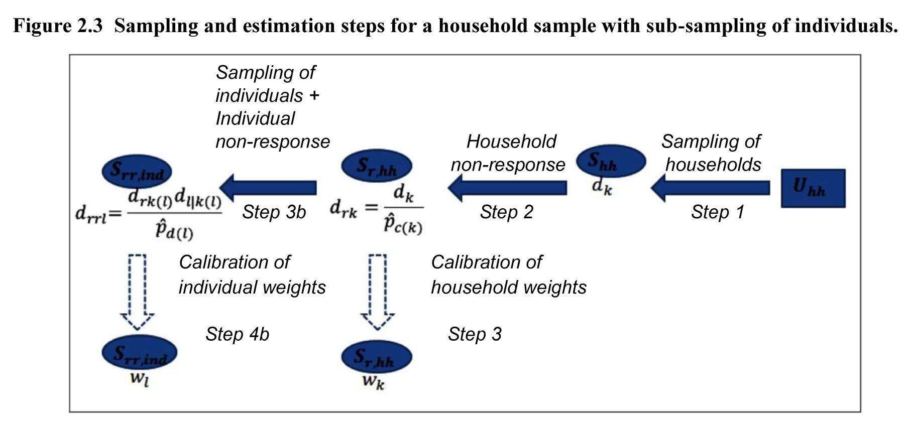
Description for Figure 2.3
Figure summarizing Sections 2.2.1
to 2.2.3, i.e., sampling and estimation steps for a household sample with
sub-sampling of individuals. The first step consists in randomly selecting a
sample, denoted
from a population, denoted
by means of a stratified one-stage sampling
design. Each unit of this sample has a survey weights, denoted
The second step consists in the treatment of
the non-response in the selected sample. The survey weights are adjusted to take
into account the non-response, now, denoted
In the third, the weights adjusted for
non-response are calibrated on auxiliary totals known on the population,
finally denoted
At step 3b, the sub-sampling of individuals
from the selected households is done, as well as the treatment for individuals’
non-response. Individuals’ survey weights adjusted for non-response are denoted
Finally, at step 4b, the individuals’ weights
adjusted for non-response are calibrated on auxiliary totals known on the
population, finally denoted
2.2.4 Computation of individual weights on an example
We continue the example initiated in Section 2.1.4.
Recall that the sample of responding households is
The set of all individuals inside the
responding households is as follows (say):
We suppose that the sampling design consists in selecting one individual
exactly inside each household. The set
of all sampled individuals inside the
responding households is
From equations (2.23) and (2.16), the individual weights corrected for
household non-response are therefore
Among these 7 selected individuals, 4 only are surveyed
due to non-response, accounted for by using the method of Response Homogeneity
Groups (RHGs). We suppose that there are two RHGs: the units
and
in the first one, and the units
and
in the second one. The units
and
are non-respondents. Inside each RHG, we
compute unweighted estimated response probabilities
This leads to
The weights accounting for household/individual non-response are obtained
for the respondents by dividing the weights in (2.32) by the estimated response
probabilities. This leads to the weights
Finally, the weights are calibrated to match the population size
and an auxiliary total
Note that, using the sample of respondents, we obtain
214.4 and
451.3. The calibrated weights are
The sampling and estimation steps are summarized in Figure 2.4.

Description for Figure 2.4
Figure summarizing Section 2.2.4,
i.e., estimation steps for the weighting of individuals with an example. The
figure illustrates with an example the steps explained in Sections 2.2.1
to 2.2.3. In this example, individuals
and
are non-respondents.
