
Assessing the coverage of confidence intervals under nonresponse. A case study on income mean and quantiles in some municipalities from the 2015 Mexican Intercensal Survey
Section 3. Empirical study based on data from the populations MIC2015_Oax and MIC2015_Oaxtrunc
The population census considered in this work consisted of 208,101 inhabitants with complete responses in a vector of six auxiliary variables: age, educational level, employment status, gender, indigenous language, and marital status. The variable of interest corresponds to the monthly income.
A logistic regression with some two-way interactions was fitted to the 208,101 observations, with response variable if an income value was given by individual and if it was not, and the vector of six explanatory variables. This model was then applied to the population of 161,296 individuals, which corresponds to those with This led to a set of response propensity values
The set of 161,296 respondents, with response propensities is referred to as MIC2015_Oax population. The distribution of income in this population is highly asymmetric partly due to the presence of some very large values. When removing the 80 observations with income larger than or equal to 50,000, we obtain a truncated population referred to as MIC2015_Oaxtrunc, which is also used in our experiments.
The step distribution function of income has only 913 and 887 jumps in each population respectively, with some large jumps at income values that are near the quantiles of interest. In particular, 2,571 accounts for 7.3% of the distribution and is very close to the quantile (1.1%) and (4.2%) are close to whereas 6,429 (2.8%) and 7,000 (1.1%) are close to
3.1 Numerical results
For each population, the coverage rate of the CI for each method was estimated as follows:
- A simple random sample of size was selected.
- For each unit with response propensity we generated from a
- Two cases were considered: a) full response and b) average nonresponse rate of 22.5%. For the latter, a logistic regression with two-way interactions, with as the response and the six explanatory variables, was selected by forward selection using the BIC criterion. The estimated response probabilities were obtained with the selected model.
- 90% CIs were computed using linearization (Lin), empirical likelihood (EL) and the Woodruff (W) method for quantiles.
- Steps 1 to 4 were repeated 5,000 times and the coverage rate for each method and for each parameter was calculated as the proportion of CIs that covered the corresponding parameter value.
Table 3.1 shows the results for 5,000. Table 3.2 shows the absolute value of the percent relative bias, with and of the percent relative root mean square error, Figure 3.1 presents the distribution of the 5,000 estimates for the nonresponse scenario for each parameter; the corresponding distributions for the full response scenario are qualitatively similar. The results for 1,000 are omitted since they were similar to those obtained with 5,000. From Tables 3.1 and 3.2 and Figure 3.1, we make the following remarks:
- For Lin and EL methods perform similarly: they have a poor performance (coverage as low as 72.9%) for MIC2015_Oax, and a good one for MIC2015_Oaxtrunc, reaching the nominal level with similar tail error rates and CI average length. Figure 3.1 a) shows that the distribution of is symmetric for MIC2015_Oaxtrunc and highly asymmetric for MIC2015_Oax; this asymmetry seems to be related to the 80 extreme income values not present in MIC2015_Oaxtrunc.
- For quantiles, Lin method has a poor performance with the shortest CI average length in both scenarios, in spite of the expected overestimation of the variance in the nonresponse scenario. This method relies on the normality of but Figures 3.1 b), c) and d) show that the distribution of is far from being symmetric and unimodal, with modes around income values with high frequency. Especially for where the coverage rate is as low as 31.4%, the distribution of is multimodal with a high proportion of values that are farther from than half the CI average length. EL and W methods generally perform well, except for in the full response scenario and for in MIC2015_Oax. The low coverages seem to be related to the observed high frequency of the two income values 2,571 (7.3%) and 6,429 (2.8%). The first one is very close to 2,570 and some of the CIs for are too narrow when 2,571. The second one is farther from in MIC2015_Oax than in MIC2015_Oaxtrunc, reducing the proportion of CIs that cover when 6,429, see Figure 3.1 d), where 6,921 in MIC2015_Oax and 6,856 in MIC2015_Oaxtrunc.
- Table 3.2 shows that the RB is small, less than 3.3%, for all parameters. When only a simple adjustment with the percentage of nonresponse is applied (not shown in this note), the RB is larger and all the methods have a very poor performance. These results suggest that the use of a propensity model helps to obtain a RB comparable with that of the full response case. For the empirical double expansion estimator is even less biased than the one associated with the full response scenario; however their RRMSE are comparable and the largest among those for the parameters of interest, since the distribution of the estimators is multimodal in both scenarios, see Figure 3.1 b).
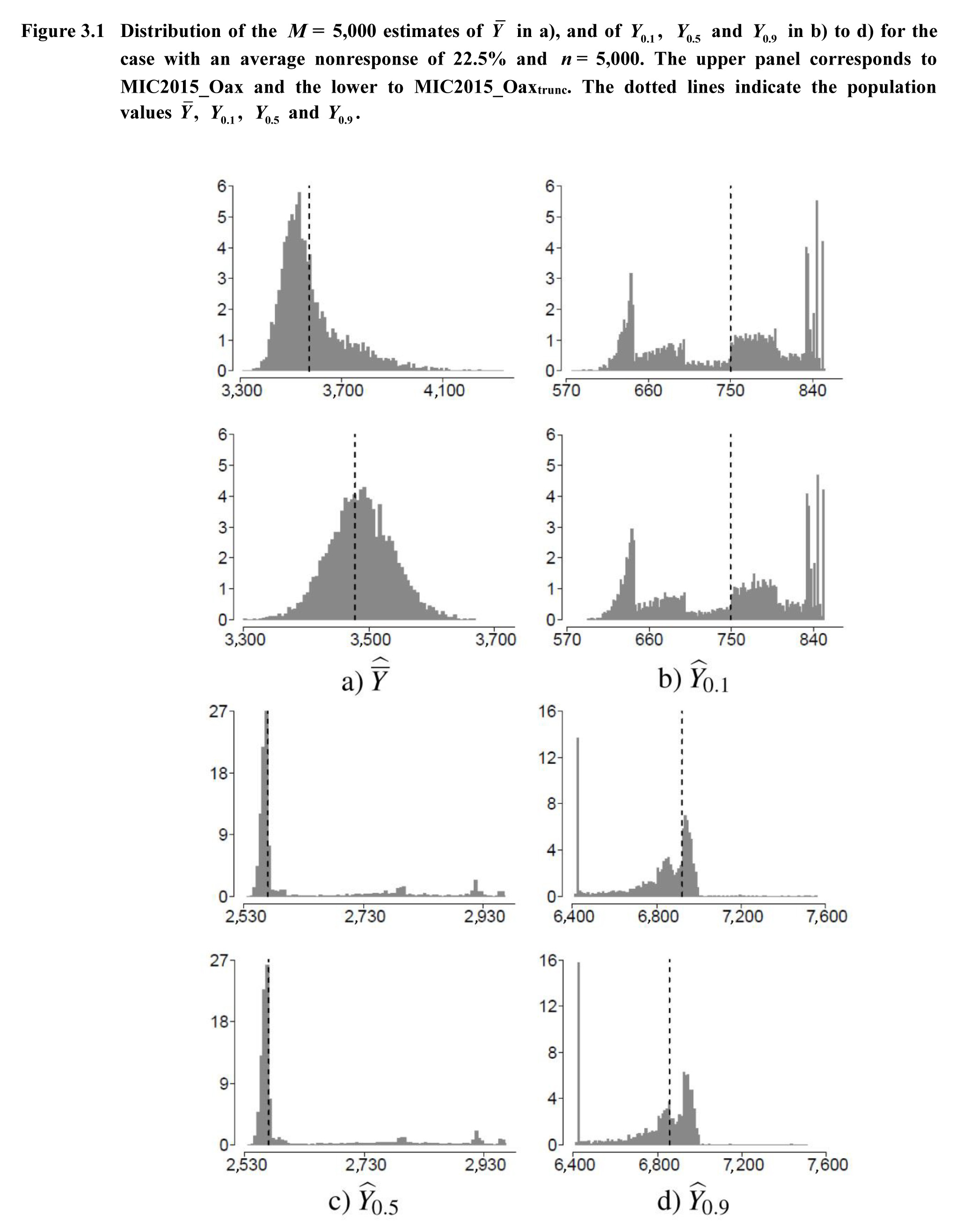
Description for Figure 3.1
Figure illustrating the distribution of the 5,000 estimates of the population mean revenue in graph a), and of the population quantiles of revenue 0.1, 0.5 and 0.9 in graphs b) to d) for the case with an average nonresponse of 22.5% and a sample size of 5,000. For graphs a) to d), the upper panel corresponds to MIC2015_Oax and the lower to MIC2015_Oaxtrunc. The dotted lines indicate the population values for each statistic being respectively estimated. The distribution of the population mean revenue estimate is symmetric for MIC2015_Oaxtrunc and highly asymmetric for MIC2015_Oax; this asymmetry seems to be related to the 80 extreme income values not present in MIC2015_Oaxtrunc. The distribution of the population quantiles of revenue estimates is far from being symmetric and unimodal, with modes around income values with high frequency.
| Parameter | Method | Coverage % | Lower tail err. rates % | Upper tail err. rates % | CI average length | ||||
|---|---|---|---|---|---|---|---|---|---|
| NR | Full | NR | Full | NR | Full | NR | Full | ||
| MIC2015_Oax | |||||||||
| EL | 79.1Note * | 72.9Note * | 4.5 | 3.8Note * | 16.4Note * | 23.3Note * | 370.8 | 335.4 | |
| Lin | 80.6Note * | 73.8Note * | 0.3Note * | 0.1Note * | 19.1Note * | 26.1Note * | 345.3 | 309.9 | |
| EL | 91.1Note * | 90.5 | 6.0Note * | 4.1Note * | 2.9Note * | 5.4 | 192.8 | 179.5 | |
| W | 90.6 | 89.8 | 6.2Note * | 4.2Note * | 3.2Note * | 6.0Note * | 191.2 | 177.1 | |
| Lin | 37.9Note * | 35.1Note * | 28.9Note * | 19.2Note * | 33.3Note * | 45.7Note * | 114.4 | 89.4 | |
| EL | 88.2Note * | 82.3Note * | 1.6Note * | 0.7Note * | 10.2Note * | 17.1Note * | 274.6 | 225.8 | |
| W | 88.0Note * | 81.0Note * | 1.7Note * | 0.7Note * | 10.3Note * | 18.3Note * | 274.4 | 224.1 | |
| Lin | 79.0Note * | 88.0Note * | 21.0Note * | 12.0Note * | 0.0Note * | 0.0Note * | 152.2 | 127.3 | |
| EL | 84.0Note * | 83.0Note * | 2.6Note * | 2.7Note * | 13.3Note * | 14.3Note * | 527.2 | 470.2 | |
| W | 86.1Note * | 84.3Note * | 2.5Note * | 2.7Note * | 11.4Note * | 13.0Note * | 533.8 | 474.2 | |
| Lin | 72.3Note * | 73.5Note * | 0.4Note * | 0.1Note * | 27.3Note * | 26.4Note * | 392.8 | 346.6 | |
| MIC2015_Oaxtrunc | |||||||||
| EL | 90.5 | 90.6 | 6.4Note * | 4.4 | 3.0Note * | 5.0 | 173.7 | 147.5 | |
| Lin | 90.8Note * | 90.1 | 5.7Note * | 4.2Note * | 3.5Note * | 5.6Note * | 171.2 | 145.0 | |
| EL | 89.8 | 89.9 | 6.8Note * | 4.0Note * | 3.4Note * | 6.1Note * | 191.7 | 178.7 | |
| W | 89.1Note * | 89.1Note * | 7.0Note * | 4.1Note * | 4.0Note * | 6.8Note * | 190.0 | 176.2 | |
| Lin | 35.5Note * | 31.4Note * | 29.4Note * | 21.0Note * | 35.1Note * | 47.6Note * | 104.9 | 81.4 | |
| EL | 87.2Note * | 80.4Note * | 1.6Note * | 0.9Note * | 11.2Note * | 18.7Note * | 267.8 | 218.5 | |
| W | 87.1Note * | 79.3Note * | 1.6Note * | 0.9Note * | 11.3Note * | 19.8Note * | 267.7 | 216.7 | |
| Lin | 80.0Note * | 87.4Note * | 20.0Note * | 12.6Note * | 0.0Note * | 0.0Note * | 144.9 | 121.0 | |
| EL | 90.3 | 90.1 | 4.4 | 4.4Note * | 5.3 | 5.5 | 521.3 | 470.8 | |
| W | 92.3Note * | 91.9Note * | 4.3Note * | 4.3Note * | 3.5Note * | 3.8Note * | 528.2 | 475.3 | |
| Lin | 75.6Note * | 77.0Note * | 0.1Note * | 0.1Note * | 24.3Note * | 23.0Note * | 411.7 | 365.5 | |
|
|||||||||
| Population | ||||||||||||||||
|---|---|---|---|---|---|---|---|---|---|---|---|---|---|---|---|---|
| RB | RRMSE | RB | RRMSE | RB | RRMSE | RB | RRMSE | |||||||||
| NR | Full | NR | Full | NR | Full | NR | Full | NR | Full | NR | Full | NR | Full | NR | Full | |
| MIC2015_Oax | 0.30 | 0.01 | 3.8 | 3.2 | 0.58 | 3.13 | 10.4 | 9.9 | 1.96 | 0.93 | 4.8 | 3.4 | 1.79 | 1.68 | 3.3 | 3.0 |
| MIC2015_Oaxtrunc | 0.27 | 0.02 | 1.5 | 1.3 | 0.71 | 3.23 | 10.5 | 10.0 | 1.87 | 0.96 | 4.8 | 3.5 | 1.05 | 0.95 | 3.0 | 2.8 |
- Date modified: