Estimating the false negatives due to blocking in record linkage
Section 6. Empirical study

• Previous
• Next

The empirical study is based on staffing data from the Public Service Resourcing System (PSRS), which is used by applicants to the federal public service in Canada. A given user may open many accounts and apply to many jobs using the same account; each account being associated with a distinct email address. To fulfill its mandate, the Public Service Commission needs to identify all accounts from a given applicant. However this is a challenge because there is no unique identifier except for a minority of applicants. Instead, for most records, the linkage must be based on the given name, the surname and the partial birthdate, which are available for all records. The partial birthdate is comprised of the day and month of birth along with the last digit of the birth year.

The empirical study is based on a subset of 126,330 records selected from the PSRS data since 2006. The selection is based on the following criteria.

• A nonmissing unique identifier.
• Nonmissing given name, surname and partial birthdate.
• Two records for each selected value of the unique identifier.

The selected records represent 63,155 distinct values of the identifier and so many distinct individuals, with two matched records per individual. These records are split into two complete and duplicate-free registers that are linked with the following blocking criteria, and without the unique identifier. A pair is selected if the partial birthdate is the same and the SOUNDEX code (Herzog et al., 2007, Chapter 11) is the same for the given name or the surname. The expected error rates are estimated with the model and compared with the actual values based on the unique identifier.

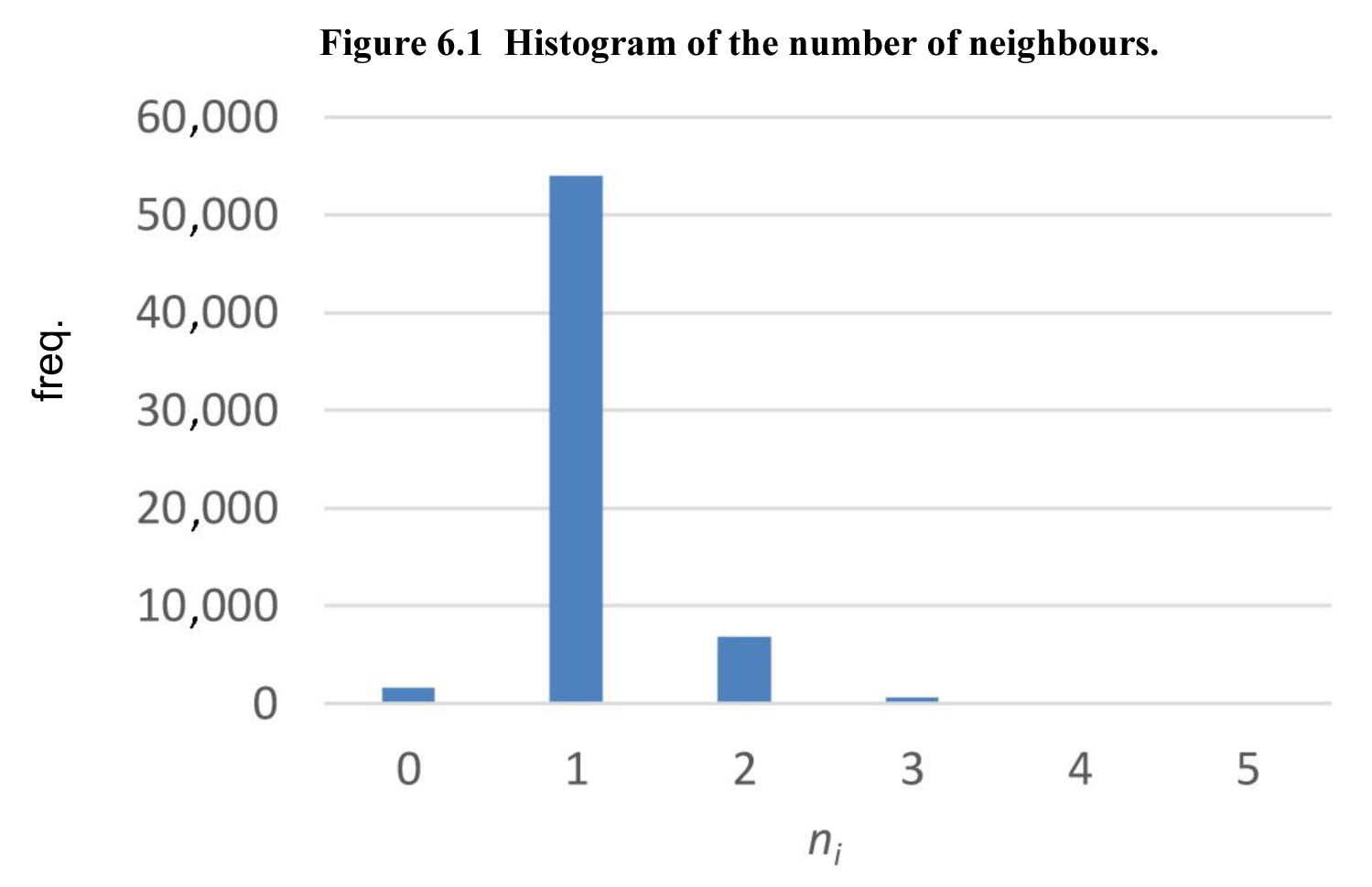
In Figure 6.1, the histogram shows that the vast majority or records have exactly one neighbour. However 1,659 records have no neighbour, while five records have five neighbours; the maximum number of neighbours of any record.

Table 6.1 cross-classifies the records by their number of neighbours and linkage errors, in agreement with Table 3.1.

The confusion matrix is as follows.

From this matrix, $\mathrm{FNR}=1,784/63,155=0.0282$ and $\text{FPR}=8,412/3.99\text{E}9=2.11\text{E}-6.$ Both measures may be viewed as the estimators $\widehat{E}[\text{FNR}]$ and $\widehat{E}[\text{FPR}]$ of their respective expectations. Since the false negative rate is the summation of independent and identically distributed random variables, its variance may be estimated by

$$\mathrm{v}\widehat{a}r(\text{FNR})=\frac{1}{N(N-1)}{\displaystyle \sum _{i=1}^N{(1-n_{i|M}-\text{FNR})}^2,}$$

based on the latent variables $n_{1|M},\dots ,n_{m|M},$ which are not directly observed in practice. As a result, the estimated FNR variance is $\mathrm{v}\widehat{a}r(\text{FNR})=4.35\text{E}-7.$ This means the estimated standard error $\widehat{S}\text{E}\left(\widehat{E}\left[\text{FNR}\right]\right)=6.6\text{E}-4$ for the estimator $\widehat{E}[\text{FNR],}$ and the 95% normal confidence interval $\widehat{E}\left[\text{FNR}\right]\mp z_{\alpha /2}\widehat{S}\text{E}\left(\widehat{E}\left[\text{FNR}\right]\right)=\left(2.82\text{E}-2\mp 1.3\text{E}-3\right)$ for the expected FNR, where $\alpha =$ 0.05 and $z_{\alpha /2}=$ 1.96. The corresponding 99% confidence interval is $(2.82\text{E}-2\mp 1.71\text{E}-3).$ Estimating the FPR variance is more difficult because the FPR involves a second order U statistic (Hoeffding, 1948; Lee, 1990). As a matter of fact, Table 6.1 does not give enough information to estimate this statistic. Estimating the variance of the model-based estimators is also challenging because the $n_i’\text{s}$ are correlated. All the point estimates are given in Table 6.3, where the first row gives the actual FNR and FPR.

The results show that the model based estimates are very close to the actual FNR and FPR when using one, two or three classes. For the false negative rate, the relative error is $100\times \left|\text{0}\text{.0303}-\text{0}\text{.0282}\right|/\text{0}\text{.0282}=\text{7}\text{.45}\%,$ while this relative error is $100\times \left|\text{2}\text{.11}-\text{2}\text{.14}\right|/\text{2}\text{.11}=\text{1}\text{.42}\%$ for the false positive rate. The small relative errors are encouraging regarding the accuracy of the proposed estimators, even if the model estimates of the expected FNR lie slightly outside the 95% confidence interval. However, the estimate belongs to the 99% confidence interval when using two classes. Choosing two classes seems optimal because the resulting estimate has the smallest relative error with respect to the actual FNR.

• Previous
• Article main page
• Next