
A grouping genetic algorithm for joint stratification and sample allocation designs
Section 3. Comparing the genetic algorithms
We now run a number of comparisons between the original GA and our GGA using publicly available datasets. Unless otherwise stated, for all the cases presented below, we adopt the following parameter setting for both genetic algorithms, where the elitism rate is 0.2, and the mutation probability is 0.05.
3.1 A comparison for the iris dataset
(Ballin and Barcaroli, 2013) use the iris dataset (Anderson, 1935; Fisher, 1936; R Core Team, 2015) to demonstrate that the GA they propose can find the optimum stratification i.e., the stratification or grouping of atomic strata which supplies the minimum sample size. The iris dataset is small and is widely available. It has 150 observations for 5 variables Sepal Length, Sepal Width, Petal Length, Petal Width and Species.
Species is a categorical variable which has three levels, setosa, versicolor and virginica, each of which have 50 observations. The remaining four variables are continuous measurements for length and width in centimetres. (Ballin and Barcaroli, 2013) select Petal Length and Petal Width as variables of interest, i.e., target variables. They select Sepal Length and Species as two auxiliary variables.
They convert Sepal Length to a categorical variable using a k-means algorithm (Hartigan and Wong, 1979) to define three clusters (i.e., 4.3 to less than 5.5, 5.5 to less than 6.5, 6.5 to 7.9). The cross product of the categorical version of Sepal Length with Species creates 9 atomic strata. However, one atomic stratum is empty because there are no corresponding values in Petal Length and Petal Width. Therefore there are 8 usable atomic strata for this example.
| Stratum | N | M1 | M2 | S1 | S2 | X1 | X2 | DOMAIN |
|---|---|---|---|---|---|---|---|---|
| [4.3; 5.5] (1)*setosa | 45 | 1.466667 | 0.244444 | 0.17127 | 0.106574 | [4.3; 5.5] (1) | setosa | 1 |
| [4.3; 5.5] (1)*versicolor | 6 | 3.583333 | 1.166667 | 0.491313 | 0.205481 | [4.3; 5.5] (1) | versicolor | 1 |
| [4.3; 5.5] (1)*virginica | 1 | 4.5 | 1.7 | 0 | 0 | [4.3; 5.5] (1) | virginica | 1 |
| [5.5; 6.5] (2)*setosa | 5 | 1.42 | 0.26 | 0.172047 | 0.08 | [5.5; 6.5] (2) | setosa | 1 |
| [5.5; 6.5] (2)*versicolor | 35 | 4.268571 | 1.32 | 0.367051 | 0.189435 | [5.5; 6.5] (2) | versicolor | 1 |
| [5.5; 6.5] (2)*virginica | 23 | 5.230435 | 1.947826 | 0.318194 | 0.28873 | [5.5; 6.5] (2) | virginica | 1 |
| [6.5; 7.9] (3)*versicolor | 9 | 4.677778 | 1.455556 | 0.193091 | 0.106574 | [6.5; 7.9] (3) | versicolor | 1 |
| [6.5; 7.9] (3)*virginica | 26 | 5.876923 | 2.107692 | 0.494825 | 0.228579 | [6.5; 7.9] (3) | virginica | 1 |
The initial atomic strata are reproduced in Table 3.1 where refers to the means for the corresponding values in each atomic stratum refers to the corresponding stratum population standard deviations. There are 4,140 possible partitionings of the 8 atomic strata. Consequently, it is possible to test within a reasonable amount of time the sample size for the entire search space using the bethel.r function. This has already been done (Ballin and Barcaroli, 2013) and the minimum sample size is known to be 11.
This test can be used to determine whether the new GA correctly finds the minimum sample size without exploring the entire search space. We use in this case. For this test the bethel.r function will search for the minimum sample size, in integers rather than real numbers. The chromosomes will then be ranked by sample size in ascending order. Accordingly the elite chromosomes are taken into the next iteration and the remaining chromosomes are generated using the recombination method for each algorithm.
We will compare the number of chromosomes generated to find the optimal stratification in the two algorithms as well as the number of iterations. Our anticipation is that the GGA should be more efficient, and thus typically find the optimal solution in fewer iterations than the GA.
The maximum number of iterations is set to 200, because using (Ballin and Barcaroli, 2013) as a guide we anticipate that both algorithms will find the correct solution in fewer iterations than this. Thus we have added a piece of code to both algorithms such that they stop when the optimal sample size, has been reached and supply the number of iterations taken to reach that point. This approach is different to that of (Ballin and Barcaroli, 2013) who report the number of times in 10 experiments the GA finds the correct solution for a given number of iterations ranging incrementally from 25 to 200. However, we feel this approach would better demonstrate that the GGA can find the correct solution in less iterations even on the small iris dataset experiment.
| (a) GA | (b) GGA | |||||
|---|---|---|---|---|---|---|
| Experiment | Iterations | Chromosomes | Experiment | Iterations | Chromosomes | |
| Number of | 1 | 14 | 228 | 1 | 11 | 180 |
| 2 | 8 | 132 | 2 | 7 | 116 | |
| 3 | 17 | 276 | 3 | 6 | 100 | |
| 4 | 40 | 644 | 4 | 22 | 356 | |
| 5 | 31 | 500 | 5 | 9 | 148 | |
| 6 | 13 | 212 | 6 | 11 | 180 | |
| 7 | 15 | 244 | 7 | 8 | 132 | |
| 8 | 9 | 148 | 8 | 7 | 116 | |
| 9 | 15 | 244 | 9 | 9 | 148 | |
| 10 | 15 | 244 | 10 | 11 | 180 | |
| 11 | 14 | 228 | 11 | 3 | 52 | |
| 12 | 8 | 132 | 12 | 9 | 148 | |
| 13 | 17 | 276 | 13 | 27 | 436 | |
| 14 | 40 | 644 | 14 | 12 | 196 | |
| 15 | 31 | 500 | 15 | 16 | 260 | |
| 16 | 13 | 212 | 16 | 6 | 100 | |
| 17 | 15 | 244 | 17 | 20 | 324 | |
| 18 | 9 | 148 | 18 | 6 | 100 | |
| 19 | 15 | 244 | 19 | 7 | 116 | |
| 20 | 15 | 244 | 20 | 6 | 100 | |
| 21 | 16 | 260 | 21 | 11 | 180 | |
| 22 | 67 | 1,076 | 22 | 7 | 116 | |
| 23 | 19 | 308 | 23 | 8 | 132 | |
| 24 | 9 | 148 | 24 | 5 | 84 | |
| 25 | 11 | 180 | 25 | 7 | 116 | |
| 26 | 20 | 324 | 26 | 5 | 84 | |
| 27 | 32 | 516 | 27 | 6 | 100 | |
| 28 | 10 | 164 | 28 | 6 | 100 | |
| 29 | 37 | 596 | 29 | 9 | 148 | |
| 30 | 9 | 148 | 30 | 6 | 100 | |
Table 3.2 provides the number of iterations (and chromosomes generated) taken to find over 30 experiments for both GAs.

Description for Figure 3.1
This figure shows the quartile diagram for the GA and GGA methods with chromosomes on the y-axis that varies from 0 to 1,100. The third quartile of the GGA method is at a similar level to the first quartile of the GA method.
Figure 3.1 provides the distribution of the number of chromosomes generated to find the optimal solution for the GA and the GGA. The boxplots indicate that the GGA typically needs to generate fewer chromosomes to find the optimum solution.
| Stratum | Y1 | Y2 | |||||
|---|---|---|---|---|---|---|---|
| N | Mean | SD | Mean | SD | Sample Size | ||
| GA | 1 | 50 | 1.462 | 0.1685 | 0.246 | 0.1026 | 2 |
| 2 | 50 | 4.26 | 0.4562 | 1.326 | 0.1911 | 3 | |
| 3 | 1 | 4.5 | 0 | 1.7 | 0 | 1 | |
| 4 | 23 | 5.2304 | 0.3112 | 1.9478 | 0.2824 | 3 | |
| 5 | 26 | 5.8769 | 0.4852 | 2.1077 | 0.2241 | 2 | |
| Total | This is an empty cell | 150 | This is an empty cell | This is an empty cell | This is an empty cell | This is an empty cell | 11 |
| GGA | 1 | 23 | 5.2304 | 0.3112 | 1.9478 | 0.2824 | 3 |
| 2 | 50 | 1.462 | 0.1685 | 0.246 | 0.1026 | 2 | |
| 3 | 26 | 5.8769 | 0.4852 | 2.1077 | 0.2241 | 2 | |
| 4 | 51 | 4.2647 | 0.4529 | 1.3333 | 0.1962 | 4 | |
| Total | This is an empty cell | 150 | This is an empty cell | This is an empty cell | This is an empty cell | This is an empty cell | 11 |
Table 3.3 provides example stratifications for the GA and GGA that both provide the optimal sample size necessary to meet precision constraints. (Ballin and Barcaroli, 2013) indicate that a number of partitionings from the total of 4,140 possible partitionings provide the minimum sample size. These range in size from 3 to 5 strata. It is seen that the GGA results in fewer, less fragmented design strata. The same tendency can be observed in the latter cases.
3.2 Swiss municipality dataset
The swissminucipalities dataset provided by (Barcaroli, 2014) refers to the Swiss municipalities in 2003. Each municipality belongs to one of seven regions which are at the NUTS-2 level, i.e., equivalent to provinces. Each region contains a number of cantons, which are administrative subdivisions. There are 26 cantons in Switzerland. The data, which was sourced from the Swiss Federal Statistical Office and is included in the sampling and SamplingStrata packages, contains 2,896 observations (each observation refers to a Swiss municipality in 2003). They comprise 22 variables, details of which can be examined in (Barcaroli, 2014).
The target estimates are the totals of the population by age class in each Swiss region. In this case, the target variables will be:
Y1: number of men and women aged between 0 and 19,
Y2: number of men and women aged between 20 and 39,
Y3: number of men and women aged between 40 and 64,
Y4: number of men and women aged 65 and over.
We consider 6 auxiliary variables, formed using the same k-means clustering method as the iris dataset example:
X1: classes of total population in the municipality. 18 categories,
X2: classes of wood area in the municipality. 3 categories,
X3: classes of area under cultivation in the municipality. 3 categories,
X4: classes of mountain pasture area in the municipality. 3 categories,
X5: classes of area with buildings in the municipality. 3 categories,
X6: classes of industrial area in the municipality. 3 categories.
There are 7 regions, which we treat as population domains of design to distinguish them from the design strata, replicating the experiment outlined in (Barcaroli, 2014). The number of non-empty atomic strata is 641 in the population. We set the minimum population size of stratum to be 2, and the maximum number of iterations to be 400. The results for Sample Size and Strata after 30 experiments each with 400 iterations are summarised in Figure 3.2 below.
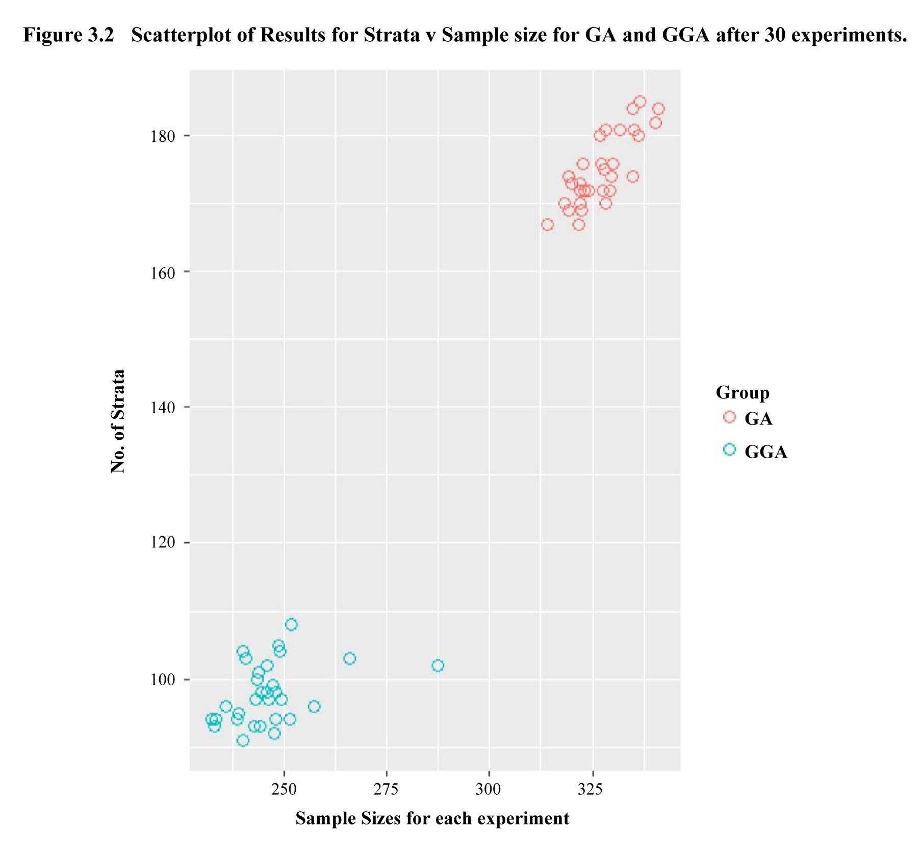
Description for Figure 3.2
This figure shows a scatter plot with the sample size on the x-axis ranging from 225 to 350 and the number of strata on the y-axis ranging from 90 to 190. The results for the 30 experiments with the GA method are in the upper right corner and those of the GGA method in the lower left corner.
Figure 3.2 clearly shows that the GGA returns a smaller sample size to the GA for these settings. The median for the GGA, 246, is 25% lower than that for the GA, 328.
3.3 2015 American Community Survey Public Use Microdata
The United States has been conducting a decennial census since 1790. In the century censuses were split into long and short form versions. A subset of the population was required to answer the longer version of the census, with the remainder answering the shorter version. After the 2000 census the longer questionnaire became the annual American Community Survey (ACS) (US Census Bureau, 2013). The 2015 ACS Public Use Microdata Sample (PUMS) file (US Census Bureau, 2016) is a sample of actual responses to the ACS representing 1% of the US population. The PUMS file contains 1,496,678 records each of which represents a unique housing unit or group quarters. There are 235 variables. The full data dictionary is available in (US Census Bureau, 2016). We selected the following to be target variables:
- household income (past 12 months),
- property value,
- selected monthly owner costs,
- fire/hazard/flood insurance (yearly amount),
and the following auxiliary variables:
- units in structure,
- tenure,
- work experience of householder and spouse,
- work status of householder or spouse in family households,
- house heating fuel,
- when structure first built.
The PUMS data for which all the values are present contains 619,747 records. We use the 51 states (based on census definitions) as domains.
In the convergence plots of Figure 3.3, the black line represents the best or lowest sample size for the chromosome population in each iteration, whereas the red line represents the mean sample size for the chromosome population in each iteration.
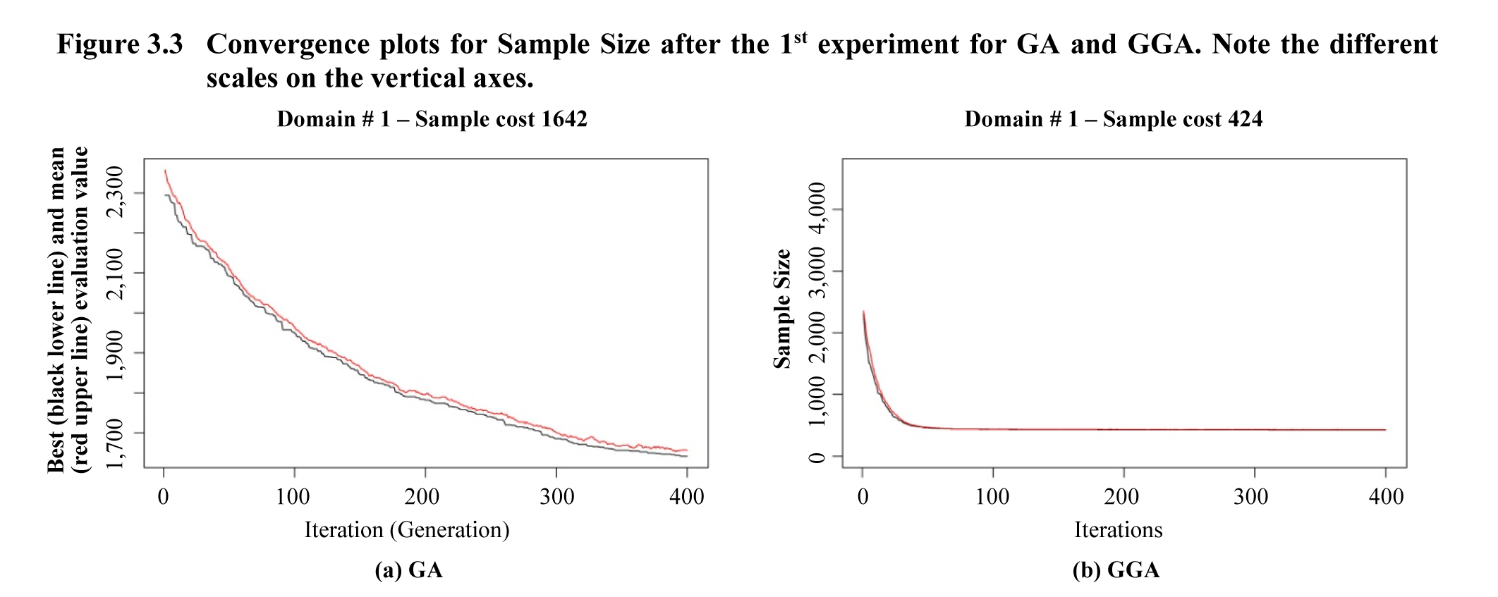
Description for Figure 3.3
This figure shows two convergence plots. The first one represents the results of the GA method with the number of iterations on the x-axis ranging from 0 to 400 and the sample sizes according to the best or mean value on the y-axis ranging from 1,700 to 2,300. Sizes are reducing according to the number of iterations without demonstrating a final convergence. The second plot represents the results of the GGA method with the number of iterations on the x-axis ranging from 0 to 400 and the sample sizes according to the optimal or mean value on the y-axis ranging from 0 to 4,000. This method converges rapidly after about 50 iterations to a value of nearly 500.
The GA appears to be reducing the sample size steadily but does not appear to have reached a local minimum after 400 iterations. The GGA appears to have reached a local or global minimum very quickly.
3.4 Kaggle Data Science for Good challenge Kiva Loans data
The online crowdfunding platform kiva.org provided a dataset of loans issued to people living in poor and financially excluded circumstances around the world over a two year period for a Kaggle Data Science for Good challenge. The dataset has 671,205 unique records. We selected these target variables:
- term in months,
- lender count,
- loan amount,
and the following auxiliary variables:
- sector,
- currency,
- activity,
- region,
- partner id,
to create atomic strata. For these variables we removed any records with missing values. We then proceeded to remove any countries with less than 10 records from the sampling frame. This resulted in a sampling frame with 614,361 records. The variable country-code defines the 73 design domains in this experiment.
| GA | GGA | Reduction | |||
|---|---|---|---|---|---|
| Sample size | Strata | Sample size | Strata | Sample size | strata |
| 78,018 | 43,030 | 11,963 | 1,793 | 84.67% | 95.83% |
Table 3.4 shows an 84.67% reduction in sample size and a 95.83% reduction in the number of strata after 100 iterations. Figure 3.4 shows that for the same starting chromosome population size for Domain 1 of the Kiva Loans dataset, the GGA attained a good sample size in less than 100 iterations, but after 10,000 iterations the GA had not converged and the sample size was still much higher than the GGA.
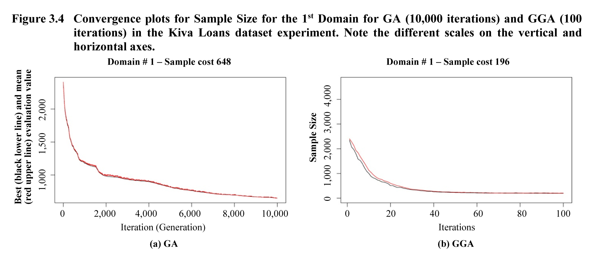
Description for Figure 3.4
This figure shows two convergence plots. The first plot represents the results of the GA method with the number of iterations on the x-axis ranging from 0 to 10,000 and the sample sizes according to the optimum or mean value on the y-axis ranging from 500 to 2,500. Sizes are reducing according to the number of iterations without demonstrating a final convergence. The second plot represents the results of the GGA method with the number of iterations on the x-axis ranging from 0 to 100 and the sample sizes according to the optimal or mean value on the y-axis ranging from 0 to 4,000. This method converges rapidly after about 50 iterations.
3.5 UN Commodity Trade Statistics data
Kaggle also hosts a copy of the UN Statistical Division Commodity Trade Statistics data. Trade records are available from 1962. We took a subset of data for the year 2011 and removed records with missing observations. This resulted in a data set with 351,057 records. We selected the following target variable:
- trade_usd
which refers to the value of trade in USD (US dollars), and the following auxiliary variables:
- commodity,
- flow,
- category.
The variable commodity is a categorical description of the type of commodity, e.g., Horses, live except pure-bred breeding. The variable flow describes whether the commodity was an import, export, re-import or re-export. The variable category describes the category of commodity, e.g., silk or fertilisers. The 171 categories of country or area were selected as domains.
| GA | GGA | Reduction | |||
|---|---|---|---|---|---|
| Sample size | Strata | Sample size | Strata | Sample size | strata |
| 288,638 | 191,000 | 84,181 | 16,555 | 70.84% | 91.33% |
3.6 2000 US census data
The Integrated Public Use Microdata Series extract is a 5% sample of the 2000 US census data (Ruggles, Genadek, Goeken, Grover and Sobek, 2017). The file contains 6,184,483 records. The US Census Data will be very similar to the ACS data as the latter is an annual version of the former. But for this experiment we selected different target and auxiliary variable combinations. The single target variable in this test is usually a key focus of household surveys:
- total household income.
We used the following information as auxiliary variables (note these are variables which are likely available in administrative data):
- annual property insurance cost,
- annual home heating fuel cost,
- annual electricity cost,
- house value.
The house value variable (VALUEH) reports the midpoint of house value intervals (e.g., 5,000 is the midpoint of the interval of less than 10,000), so we have treated it as a categorical variable. As with the 2015 ACS PUMS dataset we have taken a subset for which all values are present. This has resulted in a subset with 627,611 records. The domain for this experiment was Census region and division.
| Division | Sampling frame | GA solution | GGA solution | |||
|---|---|---|---|---|---|---|
| Sampling Units | Atomic Strata | Sample sizes | Strata | Sample sizes | Strata | |
| New England | 11,6045 | 87,084 | 81,012 | 52,628 | 376 | 58 |
| Middle Atlantic | 183,543 | 138,470 | 130,862 | 86,002 | 416 | 75 |
| East North Central | 65,480 | 58,055 | 53,075 | 35,794 | 327 | 42 |
| West North Central | 31,408 | 29,413 | 26,525 | 18,248 | 324 | 38 |
| South Atlantic | 97,189 | 83,357 | 76,716 | 51,457 | 440 | 49 |
| East South Central | 21,631 | 20,429 | 18,256 | 12,500 | 451 | 62 |
| West South Central | 22,582 | 20,919 | 18,750 | 12,730 | 407 | 39 |
| Mountain | 26,765 | 25,041 | 22,161 | 14,791 | 351 | 30 |
| Pacific | 62,968 | 54,864 | 50,136 | 33,653 | 358 | 49 |
| Total | 627,611 | 517,632 | 477,493 | 317,803 | 3,446 | 442 |
The results show a sample size of 3,446 for the GGA and a sample size of 477,493 for the GA after 100 iterations.
- Date modified: