An optimisation algorithm applied to the one-dimensional stratification problem
Section 5. Computational results
In this section, we present the results of application
of six methods to solve the stratification problem, namely: Dalenius and Hodges (DH), Geometric (GH), Kozak
(KO), Genetic Algorithm of Keskinturk and Er (KE), GRASP (GR) and the new BRKGA
method described in Section 4 (BR). All experiments where carried out
using R version 3.3.1. The methods DH, GH and KO are available from the R
package stratification of Baillargeon and Rivest (2014) (version 2.2-5). With these methods, the Neyman sample
allocation method was used. The KE method is available from the R package GA4Stratification of Er, Keskintürk and Daly (2010) (version 1.0). With this method, the
maximum number of iterations considered was 10,000 and the values of the other
parameters required were the same as those reported by Keskintürk and Er (2007), namely using
candidate solutions in each population, a
mutation rate of 15% and the sample allocation based also on the Genetic
Algorithm. Both the GR and the BR methods were implemented in R by the authors,
and the code is provided in package stratbr of de Moura Brito et al. (2017a) (version 1.2)
available from CRAN.
For the BR method,
candidate solutions were considered in each
iteration, with 20% of the solutions being made elite
and 30%
of the solutions being mutant
in each
iteration. The probability of copying a gene from the elite vector was set at
The
total number of iterations was set at 1,500. For the sample allocation, both
the BR and the GR methods were coupled with the formulation proposed by de Moura Brito
et al. (2015) which is available from the R package MultAlloc, also available from CRAN.
To compare the
relative efficiency of these methods, they were applied to 27 different
populations. Some of these populations are available from the R packages stratification and GA4Stratification, and were previously used in other comparison
studies such as Keskintürk and Er (2007), Er (2011), and de Moura Brito
et al. (2017b). Appendix A contains brief descriptions of all these
populations, including information on which variable was considered as the “
variable”
in each population. Table 5.1
provides some summaries to describe these populations.
The 27 populations
considered here form a very diverse set, with total sizes varying from a few
hundred (ME84 and P75 with
are the
smallest) to several thousand (Coffee with
is the
largest). In the size measure that matters most for efficiency of our
optimization algorithm, namely the number
of
distinct values of the stratification variable, there’s also large variation
(from
for
Kozak1 to
to Kozak3).
They also display wide variation in the asymmetry of the
variable’s distributions, ranging from
modestly negative (-0,70 for Beta103 to a substantial 40.04 for CensoCO).
All the
calculations for the computational experiment were performed using R in a
computer with 24 GB RAM, with 8 processors of 3.40 GHz (I7). Taking advantage
of the multicore architecture in modern computers, the snowfall R package was used to parallelize the BRKGA algorithm.
More specifically, at each iteration, the decoding procedure produces a set of
solutions for the boundary points. These boundary points are then supplied to
the MultAlloc package for optimum
allocation, to obtain the sample sizes in each stratum, and then to compute the
objective variance function. Since the computation time for this step is
impacted directly by the use of this global optimization formulation, the
allocation and calculation of the objective function were parallelized.
Table 5.1
Summaries of the stratification variable for the 27 populations
Table summary
This table displays the results of Summaries of the stratification variable for the 27 populations. The information is grouped by Populations (appearing as row headers), N, K, Minimum, Maximum and Skewness (appearing as column headers).
| Populations |
N |
K |
Minimum |
Maximum |
Skewness |
| AgrMinas |
844 |
226 |
5.00 |
47,800.00 |
7.32 |
| BeefFarms |
430 |
353 |
50.00 |
24,250.00 |
4.56 |
| Beta103 |
1,000 |
1,000 |
357.98 |
985.96 |
-0.70 |
| CensoCO |
9,977 |
79 |
1.00 |
911.00 |
40.04 |
| Chi5 |
1,000 |
1,000 |
0.06 |
23.43 |
1.40 |
| Coffee |
18,570 |
538 |
0.01 |
13,212.00 |
19.69 |
| Debtors |
3,369 |
1,129 |
40.00 |
28,000.00 |
6.44 |
| HHinctot |
16,025 |
224 |
1.00 |
6,900.00 |
2.71 |
| Iso2004 |
487 |
487 |
6.36 |
1,044.66 |
10.03 |
| Kozak1 |
4,000 |
51 |
72.00 |
3.00 |
1.40 |
| Kozak3 |
2,000 |
581 |
2,793.00 |
6.00 |
3.55 |
| Kozak4 |
10,000 |
5,453 |
74,400.00 |
62.00 |
4.20 |
| ME84 |
284 |
264 |
173.00 |
47,074.00 |
8.64 |
| MRTS |
2,000 |
2,000 |
1.41 |
4,863.66 |
8.61 |
| P100e10 |
1,000 |
1,000 |
73.56 |
127.32 |
-0.03 |
| P75 |
284 |
68 |
4.00 |
671.00 |
8.43 |
| Pop500 |
500 |
261 |
0.01 |
47,841.42 |
21.53 |
| Pop800 |
800 |
402 |
0.01 |
4,735.1 |
22.13 |
| pop1076 |
1,076 |
88 |
5.00 |
1,643 |
13.23 |
| pop1616 |
1,616 |
165 |
5.00 |
2,618 |
11.09 |
| pop2911 |
2,911 |
247 |
5.00 |
2,497 |
11.50 |
| REV84 |
284 |
277 |
347.00 |
59,877.00 |
7.83 |
| SugarCaneFarms |
338 |
101 |
18.00 |
280.00 |
2.26 |
| Swiss |
2,896 |
881 |
0.00 |
3,634.00 |
2.73 |
| USbanks |
357 |
200 |
70.00 |
977.00 |
2.07 |
| UScities |
1,038 |
116 |
10.00 |
198.00 |
2.87 |
| UScolleges |
677 |
576 |
200.00 |
9,623.00 |
2.45 |
All six methods considered
in the numerical experiment were applied to each of the 27 populations, for
numbers of strata
equal to
3, 4, 5 and 6. These values were used since they are often considered in
applications, as well as in similar comparative studies available in the
literature, such as Er (2011) and Gunning and Horgan (2004). We did not
consider larger values for
since
the additional gains in efficiency for
are
modest. The sample size
(i.e.,
fixed cost) was used, as in the numerical experiments of Er (2011) and Kozak and
Verma (2006).
To assess the
efficiency of the methods, the CVs of the estimator for the total of the
stratification variable
were
calculated for each population and number of strata, leading to
27 × 4 = 108 scenarios for each method. CVs were obtained
from equation (2.7) and multiplied by 100, to be presented as percentages. Table 5.2
provides the CVs attained by the six methods. The shaded cells indicate methods
providing the best solution (minimum CV) for each of 108 scenarios. The NAs in
these tables represent cases where solutions could not be obtained due to
problems of the specific stratification method or with the corresponding
allocation.
Analyzing the
results provided in Table 5.2, and in particular, the shaded cells, it is
evident that BR has excellent performance when compared to the five competitors
considered. This perception is reinforced by the plots in Figure 5.1,
where BR was compared with all competitors. Points above the straight line
represent scenarios where the method chosen for comparison is outperformed by
BR. It is evident from these plots that the three best performing methods are
GR, KO and BR.
Table 5.3
provides the percentage of times that each method produced the best solution
over the 108 scenarios. Both BR and KO display performance which is superior to
that of the other methods and have tied in the number of times that they have
achieved the best solution. DH produced the best solution for only three of the
108 scenarios, and GH has never produced a best solution.
The Geometric
method GH, besides leading to high CVs, also often provided infeasible
solutions, where the stratum limits lead to allocations where sample sizes were
larger than the corresponding population sizes. This method also sometimes
partitioned the population such that there were very few population elements in
some strata. According to Gunning
and Horgan (2004), and as noted by Keskintürk and Er (2007), since the interval
widths increase geometrically, the GH method will not perform well when the
stratification variable has small values, since this will lead to some narrow
strata. This method is also not applicable when the smallest value in the
stratification variable is zero.
For most
populations, the KE method has produced CVs close to those obtained by the KO,
GR and BR methods, which are the most efficient in terms of computing time. Large
variation on computing time was observed between different methods. The KE
method showed the worst results in this criterion, having displayed computing
times much larger than those of the competing methods. The KO method, on the
other hand, was the fastest in terms of computing time, while at the same time
often achieving the best possible precision (lowest CV). The BR method showed
computing time in between those of the KO and KE methods.
The graph in
Figure 5.2 shows the percentages of times that each of the methods BR, KO,
KE and GR produced the best solution, separated by number of strata. It shows a
clear advantage of the BR method when compared to the KE and GR methods. When
compared to KO, BR performed better for
and
while KO
was the winner for
and
GR
performed as well as KO for
and
but was
outperformed by both BR and KO for
and
KE was
the clear loser in this analysis, for any number of strata
We have also
searched for associations between performance and other potential drivers, such
as the skewness or the size
or
of the
populations, but have not found any meaningful association within our limited
set of populations.
Table 5.2
CVs for the estimator of total of the stratification variable by scenario
Table summary
This table displays the results of CVs for the estimator of total of the stratification variable by scenario. The information is grouped by Populations (appearing as row headers), H, CVDH, CVGH, CVKO, CVKE, CVGR and CVBR (appearing as column headers).
| Populations |
H |
CVDH |
CVGH |
CVKO |
CVKE |
CVGR |
CVBR |
| AgrMinas |
3 |
4.158 |
7.187 |
4.050 |
4.089 |
4.050 |
4.050 |
| 4 |
2.714 |
4.965 |
2.643 |
2.811 |
2.645 |
2.645 |
| 5 |
2.325 |
3.828 |
1.945 |
2.262 |
1.945 |
1.945 |
| 6 |
1.821 |
2.975 |
1.593 |
1.932 |
1.580 |
1.580 |
| BeefFarms |
3 |
2.758 |
2.491 |
1.875 |
2.086 |
1.875 |
1.875 |
| 4 |
1.853 |
1.825 |
1.188 |
1.557 |
1.188 |
1.188 |
| 5 |
1.455 |
1.369 |
0.902 |
1.280 |
0.902 |
0.902 |
| 6 |
1.148 |
1.167 |
0.726 |
0.990 |
0.726 |
0.726 |
| Beta103 |
3 |
0.561 |
0.810 |
0.560 |
0.560 |
0.559 |
0.559 |
| 4 |
0.413 |
0.579 |
0.410 |
0.408 |
0.410 |
0.410 |
| 5 |
0.337 |
0.500 |
0.329 |
0.329 |
0.329 |
0.329 |
| 6 |
0.280 |
0.418 |
0.276 |
0.275 |
0.277 |
0.276 |
| CensoCO |
3 |
NA |
4.839 |
4.334 |
4.336 |
4.334 |
4.334 |
| 4 |
NA |
4.388 |
3.078 |
3.062 |
3.078 |
3.078 |
| 5 |
NA |
NA |
2.401 |
2.435 |
2.401 |
2.401 |
| 6 |
NA |
NA |
1.949 |
1.956 |
1.943 |
1.943 |
| Chi5 |
3 |
2.522 |
4.217 |
2.502 |
2.489 |
2.502 |
2.502 |
| 4 |
1.897 |
3.199 |
1.889 |
1.881 |
1.889 |
1.889 |
| 5 |
1.518 |
2.875 |
1.515 |
1.538 |
1.515 |
1.515 |
| 6 |
1.258 |
NA |
1.248 |
1.251 |
1.248 |
1.248 |
| Coffe |
3 |
10.049 |
12.598 |
6.906 |
6.876 |
6.906 |
6.906 |
| 4 |
NA |
10.450 |
4.996 |
5.027 |
4.996 |
4.996 |
| 5 |
NA |
8.124 |
3.877 |
3.939 |
3.877 |
3.877 |
| 6 |
NA |
6.756 |
3.176 |
3.477 |
3.176 |
3.176 |
| Debtors |
3 |
5.626 |
6.150 |
5.554 |
5.554 |
5.554 |
5.554 |
| 4 |
4.098 |
4.387 |
4.049 |
4.049 |
4.049 |
4.049 |
| 5 |
3.163 |
3.595 |
3.131 |
3.131 |
3.131 |
3.131 |
| 6 |
2.639 |
2.897 |
2.562 |
2.562 |
2.562 |
2.562 |
| HHinctot |
3 |
3.206 |
5.106 |
3.184 |
3.184 |
3.184 |
3.184 |
| 4 |
2.436 |
4.542 |
2.429 |
2.430 |
2.429 |
2.429 |
| 5 |
1.993 |
4.225 |
1.973 |
1.979 |
1.973 |
1.973 |
| 6 |
1.676 |
3.794 |
1.629 |
1.629 |
1.629 |
1.629 |
| Iso2004 |
3 |
2.716 |
3.330 |
1.894 |
1.894 |
1.894 |
1.894 |
| 4 |
2.059 |
2.154 |
1.206 |
1.206 |
1.207 |
1.207 |
| 5 |
1.616 |
1.839 |
0.908 |
0.908 |
0.909 |
0.909 |
| 6 |
1.380 |
NA |
0.702 |
0.703 |
0.704 |
0.703 |
| Kozak1 |
3 |
1.695 |
2.432 |
1.695 |
1.695 |
1.695 |
1.695 |
| 4 |
1.305 |
2.020 |
1.301 |
1.301 |
1.301 |
1.301 |
| 5 |
1.051 |
1.705 |
1.050 |
1.052 |
1.050 |
1.050 |
| 6 |
0.904 |
1.402 |
0.890 |
0.917 |
0.890 |
0.890 |
| Kozak3 |
3 |
3.673 |
5.049 |
3.663 |
3.659 |
3.663 |
3.663 |
| 4 |
2.733 |
3.980 |
2.723 |
2.724 |
2.723 |
2.723 |
| 5 |
2.208 |
3.199 |
2.178 |
2.231 |
2.178 |
2.178 |
| 6 |
1.823 |
2.733 |
1.817 |
1.827 |
1.819 |
1.817 |
| Kozak4 |
3 |
4.263 |
5.811 |
4.257 |
4.239 |
4.257 |
4.257 |
| 4 |
3.219 |
4.696 |
3.204 |
3.193 |
3.205 |
3.204 |
| 5 |
2.606 |
3.873 |
2.589 |
2.587 |
2.591 |
2.589 |
| 6 |
2.168 |
3.236 |
2.155 |
2.155 |
2.157 |
2.158 |
| ME84 |
3 |
1.703 |
2.527 |
1.296 |
1.296 |
1.296 |
1.296 |
| 4 |
1.402 |
1.642 |
0.870 |
0.870 |
0.870 |
0.870 |
| 5 |
1.050 |
1.549 |
0.661 |
0.661 |
0.661 |
0.661 |
| 6 |
0.907 |
1.213 |
0.521 |
0.577 |
0.521 |
0.521 |
| MRTS |
3 |
4.363 |
5.829 |
4.167 |
4.167 |
4.167 |
4.167 |
| 4 |
3.406 |
5.259 |
2.960 |
2.960 |
2.961 |
2.960 |
| 5 |
2.498 |
4.015 |
2.297 |
2.485 |
2.297 |
2.297 |
| 6 |
2.167 |
3.445 |
1.836 |
1.836 |
1.838 |
1.836 |
| P100e10 |
3 |
0.375 |
0.444 |
0.373 |
0.371 |
0.373 |
0.373 |
| 4 |
0.295 |
0.346 |
0.294 |
0.294 |
0.294 |
0.294 |
| 5 |
0.236 |
0.288 |
0.236 |
0.236 |
0.236 |
0.236 |
| 6 |
0.198 |
0.242 |
0.196 |
0.198 |
0.196 |
0.196 |
| P75 |
3 |
1.635 |
2.592 |
1.459 |
1.459 |
1.459 |
1.459 |
| 4 |
1.415 |
1.798 |
0.966 |
0.966 |
0.966 |
0.966 |
| 5 |
1.047 |
1.563 |
0.829 |
0.835 |
0.713 |
0.713 |
| 6 |
0.896 |
1.250 |
0.769 |
0.553 |
0.552 |
0.552 |
| pop1076 |
3 |
4.597 |
3.715 |
2.437 |
2.775 |
2.437 |
2.437 |
| 4 |
NA |
2.853 |
1.624 |
2.164 |
1.624 |
1.624 |
| 5 |
NA |
2.168 |
1.204 |
1.869 |
1.203 |
1.203 |
| 6 |
NA |
1.827 |
0.953 |
1.549 |
0.951 |
0.951 |
| pop1616 |
3 |
4.989 |
4.318 |
3.898 |
3.921 |
3.898 |
3.898 |
| 4 |
3.823 |
3.267 |
2.564 |
2.716 |
2.564 |
2.564 |
| 5 |
3.187 |
2.508 |
1.882 |
2.183 |
1.882 |
1.882 |
| 6 |
NA |
2.050 |
1.527 |
1.962 |
1.496 |
1.496 |
| pop2911 |
3 |
5.925 |
5.935 |
5.605 |
5.569 |
5.605 |
5.605 |
| 4 |
4.070 |
3.992 |
3.807 |
3.807 |
3.807 |
3.807 |
| 5 |
3.262 |
3.183 |
2.918 |
2.943 |
2.918 |
2.918 |
| 6 |
2.632 |
2.649 |
2.281 |
2.418 |
2.281 |
2.281 |
| Pop500 |
3 |
NA |
0.678 |
0.092 |
0.127 |
0.092 |
0.092 |
| 4 |
NA |
0.178 |
0.059 |
0.082 |
0.060 |
0.060 |
| 5 |
NA |
0.194 |
0.043 |
0.059 |
0.045 |
0.046 |
| 6 |
NA |
0.117 |
0.033 |
0.046 |
0.036 |
0.037 |
| Pop800 |
3 |
NA |
3.133 |
1.555 |
2.448 |
1.555 |
1.555 |
| 4 |
NA |
2.755 |
0.996 |
1.511 |
0.996 |
0.996 |
| 5 |
NA |
1.620 |
0.701 |
1.261 |
0.702 |
0.702 |
| 6 |
NA |
1.436 |
0.546 |
0.823 |
0.550 |
0.548 |
| REV84 |
3 |
1.901 |
2.777 |
1.614 |
1.776 |
1.614 |
1.614 |
| 4 |
1.500 |
1.975 |
1.120 |
1.120 |
1.120 |
1.120 |
| 5 |
1.235 |
1.700 |
0.835 |
0.836 |
0.835 |
0.835 |
| 6 |
0.881 |
1.315 |
0.666 |
0.666 |
0.667 |
0.666 |
| SugarCaneFarms |
3 |
1.640 |
1.929 |
1.627 |
1.628 |
1.627 |
1.627 |
| 4 |
1.152 |
1.440 |
1.118 |
1.122 |
1.118 |
1.118 |
| 5 |
0.912 |
1.186 |
0.839 |
0.858 |
0.839 |
0.839 |
| 6 |
0.707 |
1.041 |
0.691 |
0.732 |
0.682 |
0.682 |
| Swiss |
3 |
3.726 |
NA |
3.682 |
3.683 |
3.690 |
3.682 |
| 4 |
2.830 |
NA |
2.781 |
2.781 |
2.787 |
2.781 |
| 5 |
2.246 |
NA |
2.227 |
2.549 |
2.232 |
2.228 |
| 6 |
1.905 |
NA |
1.860 |
1.880 |
1.864 |
1.860 |
| USbanks |
3 |
1.861 |
1.843 |
1.802 |
1.802 |
1.802 |
1.802 |
| 4 |
1.364 |
1.417 |
1.270 |
1.270 |
1.270 |
1.270 |
| 5 |
1.118 |
1.079 |
0.861 |
0.861 |
0.861 |
0.861 |
| 6 |
0.794 |
0.850 |
0.718 |
0.710 |
0.710 |
0.710 |
| UScities |
3 |
2.738 |
2.705 |
2.655 |
2.687 |
2.655 |
2.655 |
| 4 |
1.972 |
1.951 |
1.927 |
1.934 |
1.927 |
1.927 |
| 5 |
1.483 |
1.451 |
1.436 |
1.437 |
1.436 |
1.436 |
| 6 |
1.260 |
1.305 |
1.228 |
1.214 |
1.209 |
1.209 |
| UScolleges |
3 |
2.928 |
3.169 |
2.749 |
2.749 |
2.749 |
2.749 |
| 4 |
2.106 |
2.185 |
2.018 |
2.018 |
2.018 |
2.018 |
| 5 |
1.707 |
1.838 |
1.606 |
1.607 |
1.607 |
1.606 |
| 6 |
1.486 |
1.488 |
1.323 |
1.323 |
1.323 |
1.323 |
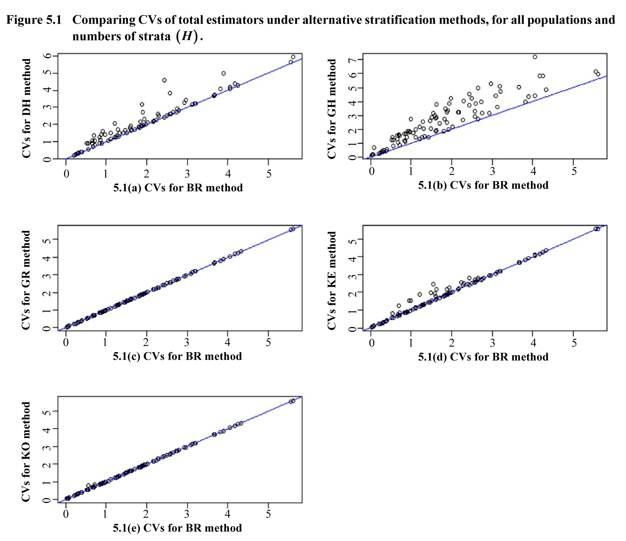
Description for Figure 5.1
Figure comparing the CVs of total
estimators under alternative stratification methods, for all populations and
number of strata. There are five scatter plots with a 45° straight line. The
CVs for BR method is on the x-axis, ranging from 0 to 5. CVs for DH, GH, GR, KE
and KO methods are on the y-axis for graphs (a) to (e) respectively, ranging
from 0 to 5 (GR, KE and KO), 0 to 6 (DH) or 0 to 7 (GH). CVs for DH and GH
methods are generally above the straight line, meaning that BR performs better.
CVs for KE method are on the line or mildly above. GR and KO’s CVs seem to be
equivalent to BR’s CVs.
Table 5.3
Percentage of times that method produced the best solution
Table summary
This table displays the results of Percentage of times that method produced the best solution. The information is grouped by Method (appearing as row headers), % Times best (appearing as column headers).
| Method |
% Times best |
| DH |
2.8 |
| GH |
0.0 |
| KE |
42.6 |
| GR |
71.3 |
| KO |
78.7 |
| BR |
78.7 |

Description for Figure 5.2
Histogram
of percentages of best solutions yielded, by method and number of strata. The
optimal solution in percentages, from 0 to 100, is on the y-axis. The number of
strata
is on the x-axis. For each
there is a bar for BR, KO, KE and GR methods.
BR method gives better results than KE and GR methods. BR method performs
better than KO method for
and
but KO wins for
and
GR performs as well as KO for
and
but is outperformed by both BR and KO for
and
KE has the worst performance for any number of
strata
ISSN : 1492-0921
Editorial policy
Survey Methodology publishes articles dealing with various aspects of statistical development relevant to a statistical agency, such as design issues in the context of practical constraints, use of different data sources and collection techniques, total survey error, survey evaluation, research in survey methodology, time series analysis, seasonal adjustment, demographic studies, data integration, estimation and data analysis methods, and general survey systems development. The emphasis is placed on the development and evaluation of specific methodologies as applied to data collection or the data themselves. All papers will be refereed. However, the authors retain full responsibility for the contents of their papers and opinions expressed are not necessarily those of the Editorial Board or of Statistics Canada.
Submission of Manuscripts
Survey Methodology is published twice a year in electronic format. Authors are invited to submit their articles in English or French in electronic form, preferably in Word to the Editor, (statcan.smj-rte.statcan@canada.ca, Statistics Canada, 150 Tunney’s Pasture Driveway, Ottawa, Ontario, Canada, K1A 0T6). For formatting instructions, please see the guidelines provided in the journal and on the web site (www.statcan.gc.ca/SurveyMethodology).
Note of appreciation
Canada owes the success of its statistical system to a long-standing partnership between Statistics Canada, the citizens of Canada, its businesses, governments and other institutions. Accurate and timely statistical information could not be produced without their continued co-operation and goodwill.
Standards of service to the public
Statistics Canada is committed to serving its clients in a prompt, reliable and courteous manner. To this end, the Agency has developed standards of service which its employees observe in serving its clients.
Copyright
Published by authority of the Minister responsible for Statistics Canada.
© Her Majesty the Queen in Right of Canada as represented by the Minister of Industry, 2019
Use of this publication is governed by the Statistics Canada Open Licence Agreement.
Catalogue No. 12-001-X
Frequency: Semi-annual
Ottawa
