
Variance estimation in multi-phase calibration
Section 4. A simulation study
The main objective of our analysis in this paper was to provide a consistent estimator for the variance of multi-phase calibrated estimators that holds for any number of phases of calibration. A simulation study could thus be executed to compare the innovative estimator with others found in the literature. As generally no alternative estimators are found for schemes with three or more phases we conducted the comparison mainly for the most investigated case of two phases. Another study was preformed for to evaluate the deviation of the proposed estimator from the true simulated value. The studies are described here in general terms. They meant basically to demonstrate the relevancy of the proposed estimator, its concurrence with the “boundary condition” of two phases and its potential for designs with more than two phases. An extensive study to characterize the efficiency of the proposed estimator as a function of the design parameters such as the sampling rates, the choice of calibrating variables and their correlation with etc., is left for future research.
An estimation process of two-phase calibration was applied to data from a recent survey on career and mobility of Doctorate Holders’ (DHs). As there exists no frame of DHs, data about higher education was extracted from a recent population census. However, only a sample that constitutes one fifth of the households enumerated in the census were given an elaborated questionnaire that includes also questions about higher education. A subsample from was drawn for the DHs survey in which a further elaborated questionnaire was given to those who were in fact DHs. Thus, a two-phase calibration scheme to estimate characteristics of DHs was in order. The first phase calibrated the joint variables of and to estimated totals computed from In the second phase, demographic data of was calibrated to the known totals from the full population register We conducted a simulation study on that data where the survey data served in our study as the true population. One thousand samples (realizations) of sizes 1,000, 200, 50 were randomly drawn from the dataset of DHs. To each sample we applied the same process of two-phase calibration utilizing the estimator given by (3.7) with equation (3.6) as a presentation of the calibrated weights and its variance estimator given by (3.11) as a special case of (3.8). As already indicated, when the estimates are identical either under the new presentation or under the conventional one used so far in the literature, Särndal et al. (1992) so our focus was on the variance estimators (3.10) and (3.11) computed according to the two different methods. A typical pattern of the comparison between the two variance estimators in this special case of two-phase calibration is presented in Figure 4.1. It can be seen that although the fundamental difference between the two variance estimators, in most realizations, the difference between their estimates is quite small. Though on a certain one it can reach up to 20%. For that particular variable shown in the figure, the mean value of both estimators for the variance was very similar, namely, 54.172 and 54.652, while the true value in the simulation data was 54.462. Even the variance of their standard deviation estimator, namely, 5.732 versus 5.932 were almost the same for that variable. These results are reported in Table 4.1. The favorable characteristic of the proposed estimator stands out in the column. Contrary to the conventional estimator where the two terms of the variance estimator are of the same order of magnitude, the term of (3.11) constitutes over 99% of the variance, with a variation of less than two percent between all 1,000 realizations. We discussed the explanation to this phenomenon in 3.2. The outcomes reported above repeated themselves for all variables studied and we found it irrelevant at this point to present other variables or investigate this specific data or the special case of two-phase calibration any further.
| Variable | Mean value | Std | CI coverage | 2nd term as percent of |
|---|---|---|---|---|
| 200.43 | 54.46 | This is an empty cell | This is an empty cell | |
| 54.65 | 5.93 | 95.2% | 77% ± 7% | |
| 54.17 | 5.73 | 95.1% | 99% ± 2% |
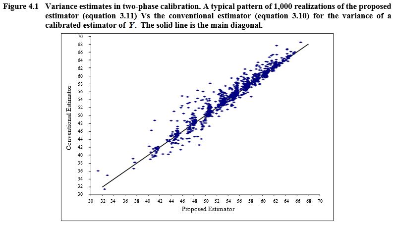
Description for Figure 4.1
Scatter plot showing the relationship between two variance estimators in two-phase calibration. The conventional estimator is on the y-axis, going from 30 to 70. The proposed estimator is on the x-axis, going from 30 to 70. A solid line representing the main diagonal goes through the scatter plot. The graph shows that in most realizations, the difference between the two estimates is quite small, even if it can reach up to 20% for some of them. The relationship between the two variances seems linear.
The similarity in estimates of the two variance estimators in the case of two phases is reassuring but a comparison in three or more phases could not be preformed because an alternative estimator to the variance does not exist. A replication method for two-phase stratified sampling was proposed by Kim et al. (2006) and a sketch for a generalization for a three-phase case is briefly outlined but with no explicit formulation or simulation results. In our simulation we added a third calibration phase using some variables, expertise field related, common with the second phase sample of DHs and conducted the study in the same manner as with the two-phase case. The simulation study has again demonstrated an excellent estimation for the variance of a three-phase calibrated estimator for all variables examined and all different sets of calibrating variables in all phases. Rapid convergence rates of the variance estimator are displayed even for very small sample sizes such as 25 or lower at the third phase. Some results for various design parameters are reported in Table 4.2. As portrayed earlier the simulation was performed over a population size of 1,000 so the first three designs have overall weight of 40 and the next three of 20. So, as expected, the variance of the calibrated estimator for the first three designs is generally higher, although it also depends on the sample sizes of the and phases as shown for example in the artificial case number 4 which depicts a generally impractical scenario. The relative biases are close to zero for all designs investigated and the 95% Confidence Interval (CI) coverages were also estimated and found to be mostly conservative and close to their nominal levels. The standard deviation of are roughly about 5% - 10% of its value as presented in column 7.
| Case | n1 | n2 | n3 | True value | of in % | 95% CI coverage | |
|---|---|---|---|---|---|---|---|
| 1 | 100 | 50 | 25 | 882.6 | 866.9 | 7.1% | 94.9% |
| 2 | 500 | 250 | 25 | 781.5 | 774.1 | 10.8% | 95.2% |
| 3 | 500 | 100 | 25 | 733.9 | 731.5 | 10.2% | 96.0% |
| 4 | 50 | 50 | 50 | 902.8 | 892.1 | 4.8% | 95.6% |
| 5 | 200 | 100 | 50 | 598.1 | 591.4 | 5.4% | 94.4% |
| 6 | 500 | 250 | 50 | 543.0 | 542.2 | 8.3% | 96.3% |
| 7 | 333 | 100 | 33 | 650.8 | 654.4 | 8.6% | 95.3% |
- Date modified: