State space time series modelling of the Dutch Labour Force Survey: Model selection and mean squared errors estimation
Section 6. Concluding remarks

Table of contents

There is a gradually increasing interest among NSIs in the use of STS models for the production of monthly figures on the labour force. In the Netherlands, such a model has been applied in the production of official LFS figures since 2010. STS models constitute a type of small area estimation (SAE), where sample information from preceding periods is used to obtain more precise estimates, as well as to account for the rotating panel design, often used in Labour Force Surveys.

Ignoring the hyperparameter uncertainty in the MSEs of STS model-based estimates results in underestimation of the MSEs of domain estimates. Particularly when series are short, which is often the case at NSIs, the bias due to ignoring hyperparameter uncertainty can be substantial. Most applications of SAE procedures in the literature are based on multilevel models, where it is common practice to account for hyperparameter uncertainty. The literature on STS models applied in the context of SAE is rather limited, with most applications ignoring hyperparameter uncertainty in the MSE estimates. Whether the bias in the obtained MSEs becomes substantial, depends on the structure of the model and on the length of the series. The present work describes a Monte-Carlo simulation applied to the STS model used by Statistics Netherlands for estimating monthly unemployment. The simulation serves two purposes. Firstly, it establishes the amount of bias in the DLFS MSEs when hyperparameter uncertainty is ignored. In addition to that, several MSE estimation methods available in the literature for the STS framework are compared in this simulation, and the best approach for the Dutch LFS is established. Secondly, simulating the distributions of the hyperparameter estimators is useful for obtaining better insights into the dynamics of the unobserved components in the STS model, and thus, ascertain the necessity to model the components as time-variant. In the case of the DLFS, the simulation shows that it might be worth considering a more restricted version of the model, where the rotation group bias is time-invariant and the population white noise is ignored. For both reasons, it is advisable to conduct a simulation as described in this paper as part of the model implementation process into official statistical production.

The comparison of the MSE estimation procedures also sheds new light on their properties. The asymptotic approximation is not applicable to cases where hyperparameters are close to zero because the information matrix of the hyperparameter estimates becomes (almost) singular. The non-parametric bootstraps, being less dependent on normality assumptions, perform better than their parametric counterparts under both Pfeffermann and Tiller (2005) and Rodriguez and Ruiz (2012) approaches, except in very short series. The most important finding is that the PT bootstraps have positive biases and consistently outperform the RR bootstraps, where the biases are generally negative and larger (in absolute terms) than those produced by the Kalman filter. This is contrary to the claim of Rodriguez and Ruiz (2012) about the superiority of their method in short time series. Apparently, their findings are purely heuristic and are based on a simple model (random walk plus noise), while Pfeffermann and Tiller (2005) prove that their bootstrap approach produces MSE estimates with a bias of correct order.

The variances of the PT MSE estimators are larger than the variances of the RR MSE estimators. Differences between MSEs of the PT and RR MSE estimators are modest to moderate (MSEs of the RR MSE estimators are 28 to 8 percent lower than those of the PT estimators, depending on the model and the time series length). More importantly, the tendency of the RR MSE estimators to have negative biases, sometimes exceeding those of the Kalman filter, renders these bootstrap methods inapplicable. Hence, the $PT -$ methods should be generally considered for other survey data too, despite the fact that these methods may occasionally be outperformed by the $RR -$ methods.

For very short time series, the non-parametric bootstraps do not seem to be an option for a model of the presented complexity. The PT parametric bootstrap, however, corrects the negatively biased MSE up to a small positive bias (1.4 to 4.4 percent, depending on the model). For the present series length of 114 months, the negative MSE bias can be reduced from about -2.4 to 1.9 percent with the non-parametric method of Pfeffermann and Tiller (2005) in the model with a time-invariant RGB. The true Kalman filter root MSEs are about 20 smaller than the standard errors of the GREG estimates in all the four models applied to the DLFS data. In general, the biases in the Kalman filter MSE estimates are relatively small in the DLFS application. Therefore, it may be deemed sufficient to rely on these naive MSE estimates for publication purposes.

Acknowledgements

We thank the National Statistical Office of the Netherlands, Statistics Netherlands, for funding this research, as well as the Associate Editor and the two anonymous reviewers for careful reading of this manuscript and valuable comments. The views expressed in this paper are those of the authors and do not necessarily reflect the policy of Statistics Netherlands.

Appendices

A. Simulated densities of the hyperparameters under the four versions of the DLFS model

This appendix presents the hyperparameter density functions obtained from simulations where the four versions of the DLFS model (see Table 5.1) act as the data generating process. The x-axes depict variance hyperparameters on a log-scale, while the y-axes stand for frequencies. The x-axis may be extended due to outliers.

Figure A.1

Description for Figure A.1

Figure showing the hyperparameter distributions under the complete DLFS model (Model 1) for eight variance hyperparameters: ${\hat{σ}}_{R}^{2},$ ${\hat{σ}}_{γ}^{2},$ ${\hat{σ}}_{λ}^{2},$ ${\hat{σ}}_{v_{t}^{t}}^{2},$ ${\hat{σ}}_{v_{t}^{t - 3}}^{2},$ ${\hat{σ}}_{v_{t}^{t - 6}}^{2},$ ${\hat{σ}}_{v_{t}^{t - 9}}^{2}$ and ${\hat{σ}}_{v_{t}^{t - 12}}^{2} .$ The normal density function with the same mean and variance is superimposed on each graph. The x-axes show the variance hyperparameters on a log-scale and the y-axes stand for frequencies. The x-axis may be extended due to outliers.

For ${\hat{σ}}_{R}^{2},$ the x-axis goes from -80 to -10 and the y-axis goes from 0 to 0.75. The values are highly concentrated around the mean creating a peak and are above the normal curve.

For ${\hat{σ}}_{γ}^{2},$ the x-axis goes from -100 to -10 and the y-axis goes from 0 to 0.075. There are extreme values at the left. The distribution is bimodal.

For ${\hat{σ}}_{λ}^{2},$ the x-axis goes from -100 to 0 and the y-axis goes from 0 to 0.2. There are extreme values at the left. The distribution is bimodal and very flat.

For ${\hat{σ}}_{v_{t}^{t}}^{2},$ the x-axis goes from -0.5 to 0.75 and the y-axis goes from 0 to 3. The distribution seems close to the normal one.

For ${\hat{σ}}_{v_{t}^{t - 3}}^{2},$ the x-axis goes from -1.0 to 0.5 and the y-axis goes from 0 to 3. The distribution seems close to the normal one.

For ${\hat{σ}}_{v_{t}^{t - 6}}^{2},$ the x-axis goes from -12.5 to 1.0 and the y-axis goes from 0 to 3. The values are highly concentrated around the mean creating a small peak.

For ${\hat{σ}}_{v_{t}^{t - 9}}^{2}$ and ${\hat{σ}}_{v_{t}^{t - 12}}^{2},$ the x-axes go from -30 to 2 and the y-axes go from 0 to 3. The values are concentrated around the mean creating a peak and are above the normal curve.

Figure A.2

Description for Figure A.2

Figure showing the hyperparameter distributions under the complete DLFS model (Model 2) for seven variance hyperparameters: ${\hat{σ}}_{R}^{2},$ ${\hat{σ}}_{λ}^{2},$ ${\hat{σ}}_{v_{t}^{t}}^{2},$ ${\hat{σ}}_{v_{t}^{t - 3}}^{2},$ ${\hat{σ}}_{v_{t}^{t - 6}}^{2},$ ${\hat{σ}}_{v_{t}^{t - 9}}^{2}$ and ${\hat{σ}}_{v_{t}^{t - 12}}^{2} .$ The normal density function with the same mean and variance is superimposed on each graph. The x-axes show the variance hyperparameters on a log-scale and the y-axes stand for frequencies. The x-axis may be extended due to outliers.

For ${\hat{σ}}_{R}^{2},$ the x-axis goes from -80 to -10 and the y-axis goes from 0 to 0.75. The values are highly concentrated around the mean creating a peak and are above the normal curve.

For ${\hat{σ}}_{λ}^{2},$ the x-axis goes from -100 to 0 and the y-axis goes from 0 to 0.3. The distribution is bimodal and the normal curve is very flat.

For ${\hat{σ}}_{v_{t}^{t}}^{2},$ the x-axis goes from -50 to 2 and the y-axis goes from 0 to 3. The values are highly concentrated around the mean creating a high peak and are above the normal curve.

For ${\hat{σ}}_{v_{t}^{t - 3}}^{2},$ the x-axis goes from -20 to 1 and the y-axis goes from 0 to 3. The values are concentrated around the mean creating a peak.

For ${\hat{σ}}_{v_{t}^{t - 6}}^{2},$ the x-axis goes from -80 to 0 and the y-axis goes from 0 to 2. The values are highly concentrated around the mean creating a high peak and are above the normal curve.

For ${\hat{σ}}_{v_{t}^{t - 9}}^{2}$ and ${\hat{σ}}_{v_{t}^{t - 12}}^{2},$ the x-axes go from -100 to 0 and the y-axes go from 0 to 2. The values are concentrated around the mean creating a high peak and are above the normal curve.

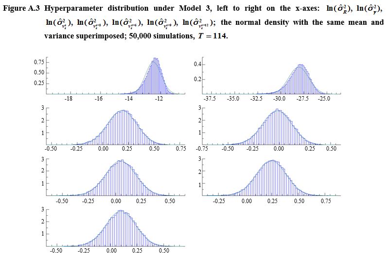
Figure A.3

Description for Figure A.3

Figure showing the hyperparameter distributions under the complete DLFS model (Model 3) for seven variance hyperparameters: ${\hat{σ}}_{R}^{2},$ ${\hat{σ}}_{γ}^{2},$ ${\hat{σ}}_{v_{t}^{t}}^{2},$ ${\hat{σ}}_{v_{t}^{t - 3}}^{2},$ ${\hat{σ}}_{v_{t}^{t - 6}}^{2},$ ${\hat{σ}}_{v_{t}^{t - 9}}^{2}$ and ${\hat{σ}}_{v_{t}^{t - 12}}^{2} .$ The normal density function with the same mean and variance is superimposed on each graph. The x-axes show the variance hyperparameters on a log-scale and the y-axes stand for frequencies.

For ${\hat{σ}}_{R}^{2},$ the x-axis goes from -18 to -10 and the y-axis goes from 0 to 0.75. The values are concentrated around the mean and asymmetric but close the normal curve.

For ${\hat{σ}}_{γ}^{2},$ the x-axis goes from -37.5 to -25 and the y-axis goes from 0 to 0.3. The values are concentrated around the mean and asymmetric but close the normal curve.

For ${\hat{σ}}_{v_{t}^{t}}^{2},$ ${\hat{σ}}_{v_{t}^{t - 3}}^{2},$ ${\hat{σ}}_{v_{t}^{t - 6}}^{2}$ and ${\hat{σ}}_{v_{t}^{t - 12}}^{2},$ the x-axes go from -0.50 to 0.50 and the y-axes go from 0 to 3. The values are very close to the normal curve.

For ${\hat{σ}}_{v_{t}^{t - 9}}^{2},$ the x-axes go from -0.25 to 0.75 and the y-axes go from 0 to 3. The values are very close to the normal curve.

Figure A.4

Description for Figure A.4

Figure showing the hyperparameter distributions under the complete DLFS model (Model 4) for six variance hyperparameters: ${\hat{σ}}_{R}^{2},$ ${\hat{σ}}_{v_{t}^{t}}^{2},$ ${\hat{σ}}_{v_{t}^{t - 3}}^{2},$ ${\hat{σ}}_{v_{t}^{t - 6}}^{2},$ ${\hat{σ}}_{v_{t}^{t - 9}}^{2}$ and ${\hat{σ}}_{v_{t}^{t - 12}}^{2} .$ The normal density function with the same mean and variance is superimposed on each graph. The x-axes show the variance hyperparameters on a log-scale and the y-axes stand for frequencies.

For ${\hat{σ}}_{R}^{2},$ the x-axis goes from -17 to -11 and the y-axis goes from 0 to 0.75. The values are concentrated around the mean and asymmetric but close the normal curve.

For ${\hat{σ}}_{v_{t}^{t}}^{2}$ and ${\hat{σ}}_{v_{t}^{t - 9}}^{2},$ the x-axes go from -0.25 to 0.75 and the y-axes go from 0 to 3. The values are very close to the normal curve.

For ${\hat{σ}}_{v_{t}^{t - 3}}^{2},$ ${\hat{σ}}_{v_{t}^{t - 6}}^{2}$ and ${\hat{σ}}_{v_{t}^{t - 12}}^{2},$ the x-axes go from -0.50 to 0.50 and the y-axes go from 0 to 3. The values are very close to the normal curve.

B. Predictive performance of the four DLFS models

Table B.1
Root mean square deviations of GREG estimates of the numbers of unemployed from their one-step-ahead predictions, per wave
Table summary
This table displays the results of Root mean square deviations of GREG estimates of the numbers of unemployed from their one-step-ahead predictions. The information is grouped by W (appearing as row headers), Model 1, Model 2, Model 3 and Model 4 (appearing as column headers).
W	Model 1			Model 2			Model 3			Model 4
W	$d =20$	$d =30$	$d =60$	$d =20$	$d =30$	$d =60$	$d =20$	$d =30$	$d =60$	$d =20$	$d =30$	$d =60$
1	34,370	33,582	34,641	34,370	33,582	34,641	34,518	33,754	34,881	34,525	33,757	34,885
2	30,130	29,770	29,410	30,130	29,770	29,410	30,138	29,780	29,418	30,144	29,779	29,409
3	35,792	32,631	34,654	35,792	32,631	34,654	35,714	32,535	34,499	35,716	32,532	34,499
4	39,647	38,556	36,797	39,647	38,556	36,797	39,753	38,640	36,891	39,743	38,633	36,889
5	38,271	37,622	36,341	38,271	37,622	36,341	38,183	37,528	36,225	38,177	37,523	36,226

References

Bailar, B. (1975). The effects of rotation group bias on estimates from panel surveys. Journal of the American Statistical Association, 70, 23-30.

Bartlett, M.S. (1946). On the theoretical specification and sampling properties of autocorrelated time-series. Supplement to the Journal of the Royal Statistical Society, 8, 27-41.

Binder, D.A., and Dick, J.P. (1990). A method for the analysis of seasonal ARIMA models. Survey Methodology, 16, 2, 239-253. Paper available at http://www.statcan.gc.ca/pub/12-001-x/1990002/article/14533-eng.pdf.

Bollineni-Balabay, O., van den Brakel, J. and Palm, F. (2016a). Multivariate state space approach to variance reduction in series with level and variance breaks due to survey redesigns. Journal of the Royal Statistical Society: Series A (Statistics in Society), 179, 377-402.

Bollineni-Balabay, O., van den Brakel, J. and Palm, F. (2016b). State space time series modelling of the Dutch Labour Force Survey: Model selection and MSE estimation, - Extended version. Discussion paper, Statistics Netherlands, Heerlen. https://www.cbs.nl/en-gb/background/2016/41/state-space-time-series.

Cochran, W. (1977). Sampling Techniques. New York: John Wiley & Sons, Inc.

Doornik, J. (2007). An Object-Oriented Matrix Programming Language Ox 5. Timberlake Consultants Press, London.

Durbin, J., and Koopman, S.J. (2002). A simple and efficient simulation smoother for state space time series analysis. Biometrika, 89, 603-615.

Durbin, J., and Koopman, S.J. (2012). Time Series Analysis by State Space Methods. Number 38. Oxford University Press.

EUROSTAT (2015). Task force on monthly unemployment - revised report. Working group labour market statistics.

Hamilton, J. (1986). A standard error for the estimated state vector of a state-space model. Journal of Econometrics, 33, 387-397.

Harvey, A. (1989). Forecasting, Structural Time Series Models and the Kalman Filter. Cambridge University Press, Cambridge.

Koopman, S.J. (1997). Exact initial kalman filtering and smoothing for nonstationary time series models. Journal of the American Statistical Association, 92, 1630-1638.

Koopman, S.J., Shephard, N. and Doornik, J. (2008). SsfPack 3.0: Statistical Algorithms for Models in State Space Form. Timberlake Consultants Press, London.

Krieg, S., and van den Brakel, J. (2012). Estimation of the monthly unemployment rate for six domains through structural time series modelling with cointegrated trends. Computational Statistics & Data Analysis, 56, 2918-2933.

Lemaître, G., and Dufour, J. (1987). An integrated method for weighting persons and families. Survey Methodology, 13, 2, 199-207. Paper available at http://www.statcan.gc.ca/pub/12-001-x/1987002/article/14607-eng.pdf.

ONS (2015). A state space model for LFS estimates: Agreeing the target and dealing with wave specific bias. Report of the 29^th meeting of the Government Statistical Service Methodology Advisory Committee. http://www.ons.gov.uk/ons/guide-method/method-quality/advisory-committee/previous-meeting-papers-and-minutes/mac-29-papers.pdf.

Pfeffermann, D. (1991). Estimation and seasonal adjustment of population means using data from repeated surveys. Journal of Business and Economic Statistics, 9, 163-175.

Pfeffermann, D. (2013). New important developments in small area estimation. Statistical Science, 28, 40-68.

Pfeffermann, D., and Rubin-Bleuer, S. (1993). Robust joint modelling of labour force series of small areas. Survey Methodology, 19, 2, 149-163. Paper available at http://www.statcan.gc.ca/pub/12-001-x/1993002/article/14458-eng.pdf.

Pfeffermann, D., and Tiller, R. (2005). Bootstrap approximation to prediction MSE for state-space models with estimated parameters. Journal of Time Series Analysis, 26, 893-916.

Pfeffermann, D., Feder, M. and Signorelli, D. (1998). Estimation of autocorrelations of survey errors with application to trend estimation in small areas. Journal of Business and Economic Statistics, 16, 339-348.

Rao, J.N.K., and Molina, I. (2015). Small Area Estimation. New York: John Wiley & Sons, Inc.

Rodriguez, A., and Ruiz, E. (2012). Bootstrap prediction mean squared errors of unobserved states based on the Kalman filter with estimated parameters. Computational Statistics and Data Analysis, 56, 62-74.

Särndal, C.-E., Swensson, B. and Wretman, J. (1992). Model Assisted Survey Sampling. Springer.

Tiller, R. (1992). Time series modelling of sample survey data from the US current population survey. Journal of Official Statistics, 8, 149-166.

van den Brakel, J., and Krieg, S. (2009). Estimation of the monthly unemployment rate through structural time series modelling in a rotating panel design. Survey Methodology, 35, 2, 177-190. Paper available at http://www.statcan.gc.ca/pub/12-001-x/2009002/article/11040-eng.pdf.

van den Brakel, J., and Krieg, S. (2015). Dealing with small sample sizes, rotation group bias and discontinuities in a rotating panel design. Survey Methodology, 41, 2, 267-296. Paper available at http://www.statcan.gc.ca/pub/12-001-x/2015002/article/14231-eng.pdf.

Zhang, M., and Honchar, O. (2016). Predicting survey estimates by state space models using multiple data sources. Paper for the Australian Bureau of Statistics’ Methodology Advisory Committee.

ISSN : 1492-0921

Editorial policy

Survey Methodology publishes articles dealing with various aspects of statistical development relevant to a statistical agency, such as design issues in the context of practical constraints, use of different data sources and collection techniques, total survey error, survey evaluation, research in survey methodology, time series analysis, seasonal adjustment, demographic studies, data integration, estimation and data analysis methods, and general survey systems development. The emphasis is placed on the development and evaluation of specific methodologies as applied to data collection or the data themselves. All papers will be refereed. However, the authors retain full responsibility for the contents of their papers and opinions expressed are not necessarily those of the Editorial Board or of Statistics Canada.

Submission of Manuscripts

Survey Methodology is published twice a year in electronic format. Authors are invited to submit their articles in English or French in electronic form, preferably in Word to the Editor, (statcan.smj-rte.statcan@canada.ca, Statistics Canada, 150 Tunney’s Pasture Driveway, Ottawa, Ontario, Canada, K1A 0T6). For formatting instructions, please see the guidelines provided in the journal and on the web site (www.statcan.gc.ca/SurveyMethodology).

Note of appreciation

Canada owes the success of its statistical system to a long-standing partnership between Statistics Canada, the citizens of Canada, its businesses, governments and other institutions. Accurate and timely statistical information could not be produced without their continued co-operation and goodwill.

Standards of service to the public

Statistics Canada is committed to serving its clients in a prompt, reliable and courteous manner. To this end, the Agency has developed standards of service which its employees observe in serving its clients.

Copyright

Published by authority of the Minister responsible for Statistics Canada.

Use of this publication is governed by the Statistics Canada Open Licence Agreement.

Catalogue No. 12-001-X

Frequency: semi-annual

Ottawa

Date modified:: 2017-06-22

Language selection

Search and menus

Search

State space time series modelling of the Dutch Labour Force Survey: Model selection and mean squared errors estimation
Section 6. Concluding remarks

Acknowledgements

Appendices

A. Simulated densities of the hyperparameters under the four versions of the DLFS model

B. Predictive performance of the four DLFS models

References

State space time series modelling of the Dutch Labour Force Survey: Model selection and mean squared errors estimation Section 6. Concluding remarks

Acknowledgements

Appendices

A. Simulated densities of the hyperparameters under the four versions of the DLFS model

B. Predictive performance of the four DLFS models

References

Editorial policy

Submission of Manuscripts

Note of appreciation

Standards of service to the public

Copyright

State space time series modelling of the Dutch Labour Force Survey: Model selection and mean squared errors estimation
Section 6. Concluding remarks