A layered perturbation method for the protection of tabular outputs
Section 2. Background

The proposed strategy aims to protect the confidentiality of tables of magnitude in a semi-controlled custom tabulation environment. It was primarily developed for administrative (census-like) data, notably personal taxation data. At Statistics Canada, such outputs are subject to disclosure control rules including minimum population sizes for identifiable geographic areas, the use of minimum-cell-size and dominance rules to suppress sensitive (confidential) cells, and the application of complementary cell suppression (CCS) to prevent the recuperation of sensitive cell values.

While personal data are inherently safer than business data, they are more readily used in custom tabulations. And with wider access to custom tabulations it becomes increasingly difficult to carry out CCS effectively. Alternative methods need to be considered. The proposed method consists of applying a perturbative technique, independently, in every non sensitive cell of every table. Only sensitive cells are suppressed, although some may become releasable if perturbed. The method is meant to protect sensitive cells in tables as well as to guard against residual disclosure from multiple tables MathType@MTEF@5@5@+= feaagKart1ev2aqatCvAUfeBSjuyZL2yd9gzLbvyNv2CaerbuLwBLn hiov2DGi1BTfMBaeXatLxBI9gBaerbd9wDYLwzYbItLDharqqtubsr 4rNCHbGeaGqk0Jf9crFfpeea0xh9v8qiW7rqqrpu0xh9Wqpm0db9Wq pepeuf0xe9q8qiYRWFGCk9vi=dbvc9s8vr0db9Fn0dbbG8Fq0Jfr=x fr=xfbpdbaqaaeaaciGaaiaabeqaamaabaabaaGcbaacbaqcLbwaqa aaaaaaaaWdbiaa=nbiaaa@3D01@ especially disclosure by the differencing of nested totals. The focus is on protecting two totals that differ by one unit.

It is assumed that we are in a semi-controlled environment where access is somewhat restricted, or at least not anonymous, so that some monitoring and control of requests is applied. This precaution is needed because offering unrestricted tabulations to anonymous hackers trying to exploit every vulnerability (in particular, through multiple requests involving carefully chosen sets of units) could lead to the approximate disclosure of unit values under certain conditions. The method is developed for census-like data, which are riskier, but it could undoubtedly be adapted to sample data if needed. The strategy is better suited to personal data as they are less subject to dominance than business data, and near-dominant cells get perturbed the most. But with some adaptation users may see to what extent the strategy could meet their needs for other types of data.

If possible, we would like the strategy to address other disclosure issues, such as the protection of ratios and of other types of outputs. Other desirable features are the ability to treat zeroes and negative values, the maintenance of data quality, the preservation of additivity in tables, and operational aspects such as computational simplicity and the use of minimal manual intervention.

In this paper we use a P MathType@MTEF@5@5@+= feaagKart1ev2aqatCvAUfeBSjuyZL2yd9gzLbvyNv2CaerbuLwBLn hiov2DGi1BTfMBaeXatLxBI9gBaerbd9wDYLwzYbItLDharqqtubsr 4rNCHbGeaGqiFu0Je9sqqrpepC0xbbL8F4rqqrFfFv0dd9Wqpe0dd9 qqaqFeFr0xbbG8FaYPYRWFb9fi0lXxbvc9Ff0dfrpe0dXdHqps0=vr 0=vr0=fdbaqaaeGaciGaaiaabeqaamaabaabaaGcbaGaamiuaiaayk W7cqGHsislaaa@3747@ percent rule to identify sensitive cell totals, meaning that a cell is sensitive if the aggregate contribution from the smallest units, starting with the third-largest, is less than P % MathType@MTEF@5@5@+= feaagKart1ev2aqatCvAUfeBSjuyZL2yd9gzLbvyNv2CaerbuLwBLn hiov2DGi1BTfMBaeXatLxBI9gBaerbd9wDYLwzYbItLDharqqtubsr 4rNCHbGeaGqiFu0Je9sqqrpepC0xbbL8F4rqqrFfFv0dd9Wqpe0dd9 qqaqFeFr0xbbG8FaYPYRWFb9fi0lXxbvc9Ff0dfrpe0dXdHqps0=vr 0=vr0=fdbaqaaeGaciGaaiaabeqaamaabaabaaGcbaGaamiuaiaacw caaaa@3578@ of the value of the largest unit (i.e., if X x 1 x 2 < P % x 1 , MathType@MTEF@5@5@+= feaagKart1ev2aqatCvAUfeBSjuyZL2yd9gzLbvyNv2CaerbuLwBLn hiov2DGi1BTfMBaeXatLxBI9gBaerbd9wDYLwzYbItLDharqqtubsr 4rNCHbGeaGqiFu0Je9sqqrpepC0xbbL8F4rqqrFfFv0dd9Wqpe0dd9 qqaqFeFr0xbbG8FaYPYRWFb9fi0lXxbvc9Ff0dfrpe0dXdHqps0=vr 0=vr0=fdbaqaaeGaciGaaiaabeqaamaabaabaaGcbaaeaaaaaaaaa8 qacaWGybGaeyOeI0IaamiEa8aadaWgaaWcbaWdbiaaigdaa8aabeaa k8qacqGHsislcaWG4bWdamaaBaaaleaapeGaaGOmaaWdaeqaaOWdbi abgYda8iaadcfacaGGLaGaaGjbVlaadIhapaWaaSbaaSqaa8qacaaI XaaapaqabaGcpeGaaiilaaaa@4215@ where X MathType@MTEF@5@5@+= feaagKart1ev2aqatCvAUfeBSjuyZL2yd9gzLbvyNv2CaerbuLwBLn hiov2DGi1BTfMBaeXatLxBI9gBaerbd9wDYLwzYbItLDharqqtubsr 4rNCHbGeaGqiFu0Je9sqqrpepC0xbbL8F4rqqrFfFv0dd9Wqpe0dd9 qqaqFeFr0xbbG8FaYPYRWFb9fi0lXxbvc9Ff0dfrpe0dXdHqps0=vr 0=vr0=fdbaqaaeGaciGaaiaabeqaamaabaabaaGcbaGaamiwaaaa@34D7@ is the cell total and x i MathType@MTEF@5@5@+= feaagKart1ev2aqatCvAUfeBSjuyZL2yd9gzLbvyNv2CaerbuLwBLn hiov2DGi1BTfMBaeXatLxBI9gBaerbd9wDYLwzYbItLDharqqtubsr 4rNCHbGeaGqiFu0Je9sqqrpepC0xbbL8F4rqqrFfFv0dd9Wqpe0dd9 qqaqFeFr0xbbG8FaYPYRWFb9fi0lXxbvc9Ff0dfrpe0dXdHqps0=vr 0=vr0=fdbaqaaeGaciGaaiaabeqaamaabaabaaGcbaGaamiEamaaBa aaleaacaWGPbaabeaaaaa@3611@ is the contribution of its i th MathType@MTEF@5@5@+= feaagKart1ev2aqatCvAUfeBSjuyZL2yd9gzLbvyNv2CaerbuLwBLn hiov2DGi1BTfMBaeXatLxBI9gBaerbd9wDYLwzYbItLDharqqtubsr 4rNCHbGeaGqiFu0Je9sqqrpepC0xbbL8F4rqqrFfFv0dd9Wqpe0dd9 qqaqFeFr0xbbG8FaYPYRWFb9fi0lXxbvc9Ff0dfrpe0dXdHqps0=vr 0=vr0=fdbaqaaeGaciGaaiaabeqaamaabaabaaGcbaGaamyAamaaCa aaleqabaGaaeiDaiaabIgaaaaaaa@36F7@ largest unit). We assume that cells failing a minimum-cell-size rule are also sensitive.

We are interested in preserving quality and confidentiality for magnitude data in a custom tabulation environment. Techniques for tables of magnitude such as CCS (Cox and Sande 1979) and Controlled Tabular Adjustment (Cox and Dandekar 2004) do not work very well in such an environment. They require solving optimization problems to find table-specific solutions. Problems start to occur when trying to protect huge, complex and/or related (i.e., linked) tables, such as the inability to reach a solution, or the use of heuristics that may yield inconsistencies in suppression or perturbation patterns that can be exploited by hackers. It is far easier to perturb cell totals directly, e.g., by the application of random noise, but one still needs to look at the microdata to ensure adequate protection while controlling the impact on quality. And without additional measures it can lead to inconsistencies within and between tables that can be exploited by hackers.

Microdata perturbation, where data are perturbed at the microdata level, is better suited for our multi-table environment. Tables are additive and usually without suppression; with consistent results between tables. If custom tables are allowed it may be possible to recover some individual perturbed values directly or by differencing, so the noise level for each unit would need to be high enough to meet target ambiguity levels. As a result, the cumulated noise for specific aggregates can be large. A microdata perturbation method developed and used at the U.S. Census Bureau is the EZS method (Evans, Zayatz and Slanta 1998). EZS multiplies individual values x i MathType@MTEF@5@5@+= feaagKart1ev2aqatCvAUfeBSjuyZL2yd9gzLbvyNv2CaerbuLwBLn hiov2DGi1BTfMBaeXatLxBI9gBaerbd9wDYLwzYbItLDharqqtubsr 4rNCHbGeaGqiFu0Je9sqqrpepC0xbbL8F4rqqrFfFv0dd9Wqpe0dd9 qqaqFeFr0xbbG8FaYPYRWFb9fi0lXxbvc9Ff0dfrpe0dXdHqps0=vr 0=vr0=fdbaqaaeGaciGaaiaabeqaamaabaabaaGcbaGaamiEamaaBa aaleaacaWGPbaabeaaaaa@3611@ by a weight w i = 1 + ε i , MathType@MTEF@5@5@+= feaagKart1ev2aqatCvAUfeBSjuyZL2yd9gzLbvyNv2CaerbuLwBLn hiov2DGi1BTfMBaeXatLxBI9gBaerbd9wDYLwzYbItLDharqqtubsr 4rNCHbGeaGqiFu0Je9sqqrpepC0xbbL8F4rqqrFfFv0dd9Wqpe0dd9 qqaqFeFr0xbbG8FaYPYRWFb9fi0lXxbvc9Ff0dfrpe0dXdHqps0=vr 0=vr0=fdbaqaaeGaciGaaiaabeqaamaabaabaaGcbaGaam4DamaaBa aaleaacaWGPbaabeaakiabg2da9iaaigdacqGHRaWkcqaH1oqzdaWg aaWcbaGaamyAaaqabaGccaGGSaaaaa@3C38@ where ε i MathType@MTEF@5@5@+= feaagKart1ev2aqatCvAUfeBSjuyZL2yd9gzLbvyNv2CaerbuLwBLn hiov2DGi1BTfMBaeXatLxBI9gBaerbd9wDYLwzYbItLDharqqtubsr 4rNCHbGeaGqiFu0Je9sqqrpepC0xbbL8F4rqqrFfFv0dd9Wqpe0dd9 qqaqFeFr0xbbG8FaYPYRWFb9fi0lXxbvc9Ff0dfrpe0dXdHqps0=vr 0=vr0=fdbaqaaeGaciGaaiaabeqaamaabaabaaGcbaGaeqyTdu2aaS baaSqaaiaadMgaaeqaaaaa@36BB@ are i.i.d. random variables with mean 0 and variance σ ε 2 . MathType@MTEF@5@5@+= feaagKart1ev2aqatCvAUfeBSjuyZL2yd9gzLbvyNv2CaerbuLwBLn hiov2DGi1BTfMBaeXatLxBI9gBaerbd9wDYLwzYbItLDharqqtubsr 4rNCHbGeaGqiFu0Je9sqqrpepC0xbbL8F4rqqrFfFv0dd9Wqpe0dd9 qqaqFeFr0xbbG8FaYPYRWFb9fi0lXxbvc9Ff0dfrpe0dXdHqps0=vr 0=vr0=fdbaqaaeGaciGaaiaabeqaamaabaabaaGcbaaeaaaaaaaaa8 qacqaHdpWCpaWaa0baaSqaa8qacqaH1oqza8aabaWdbiaaikdaaaGc paGaaiOlaaaa@3976@ Two distributions for ε i MathType@MTEF@5@5@+= feaagKart1ev2aqatCvAUfeBSjuyZL2yd9gzLbvyNv2CaerbuLwBLn hiov2DGi1BTfMBaeXatLxBI9gBaerbd9wDYLwzYbItLDharqqtubsr 4rNCHbGeaGqiFu0Je9sqqrpepC0xbbL8F4rqqrFfFv0dd9Wqpe0dd9 qqaqFeFr0xbbG8FaYPYRWFb9fi0lXxbvc9Ff0dfrpe0dXdHqps0=vr 0=vr0=fdbaqaaeGaciGaaiaabeqaamaabaabaaGcbaGaeqyTdu2aaS baaSqaaiaadMgaaeqaaaaa@36BB@ of interest are the split triangular distribution (shaped like Figure 2.1) and the split uniform distribution (shaped like Figure 2.2) whose corresponding values of σ ε 2   MathType@MTEF@5@5@+= feaagKart1ev2aqatCvAUfeBSjuyZL2yd9gzLbvyNv2CaerbuLwBLn hiov2DGi1BTfMBaeXatLxBI9gBaerbd9wDYLwzYbItLDharqqtubsr 4rNCHbGeaGqiFu0Je9sqqrpepC0xbbL8F4rqqrFfFv0dd9Wqpe0dd9 qqaqFeFr0xbbG8FaYPYRWFb9fi0lXxbvc9Ff0dfrpe0dXdHqps0=vr 0=vr0=fdbaqaaeGaciGaaiaabeqaamaabaabaaGcbaaeaaaaaaaaa8 qacqaHdpWCpaWaa0baaSqaa8qacqaH1oqza8aabaWdbiaaikdaaaGc caGGGcaaaa@39D9@ are ( 3 a 2 + 2 a b + b 2 ) / 6 MathType@MTEF@5@5@+= feaagKart1ev2aqatCvAUfeBSjuyZL2yd9gzLbvyNv2CaerbuLwBLn hiov2DGi1BTfMBaeXatLxBI9gBaerbd9wDYLwzYbItLDharqqtubsr 4rNCHbGeaGqiFu0Je9sqqrpepC0xbbL8F4rqqrFfFv0dd9Wqpe0dd9 qqaqFeFr0xbbG8FaYPYRWFb9fi0lXxbvc9Ff0dfrpe0dXdHqps0=vr 0=vr0=fdbaqaaeGaciGaaiaabeqaamaabaabaaGcbaWaaSGbaeaada qadaqaaiaaiodacaWGHbWaaWbaaSqabeaacaaIYaaaaOGaey4kaSIa aGOmaiaadggacaWGIbGaey4kaSIaamOyamaaCaaaleqabaGaaGOmaa aaaOGaayjkaiaawMcaaaqaaiaaiAdaaaaaaa@3F16@ and ( a 2 + a b + b 2 ) / 3 , MathType@MTEF@5@5@+= feaagKart1ev2aqatCvAUfeBSjuyZL2yd9gzLbvyNv2CaerbuLwBLn hiov2DGi1BTfMBaeXatLxBI9gBaerbd9wDYLwzYbItLDharqqtubsr 4rNCHbGeaGqiFu0Je9sqqrpepC0xbbL8F4rqqrFfFv0dd9Wqpe0dd9 qqaqFeFr0xbbG8FaYPYRWFb9fi0lXxbvc9Ff0dfrpe0dXdHqps0=vr 0=vr0=fdbaqaaeGaciGaaiaabeqaamaabaabaaGcbaWaaSGbaeaada qadaqaaiaadggadaahaaWcbeqaaiaaikdaaaGccqGHRaWkcaWGHbGa amOyaiabgUcaRiaadkgadaahaaWcbeqaaiaaikdaaaaakiaawIcaca GLPaaaaeaacaaIZaaaaiaacYcaaaa@3E4A@ respectively. The ε i ( or w i ) MathType@MTEF@5@5@+= feaagKart1ev2aqatCvAUfeBSjuyZL2yd9gzLbvyNv2CaerbuLwBLn hiov2DGi1BTfMBaeXatLxBI9gBaerbd9wDYLwzYbItLDharqqtubsr 4rNCHbGeaGqiFu0Je9sqqrpepC0xbbL8F4rqqrFfFv0dd9Wqpe0dd9 qqaqFeFr0xbbG8FaYPYRWFb9fi0lXxbvc9Ff0dfrpe0dXdHqps0=vr 0=vr0=fdbaqaaeGaciGaaiaabeqaamaabaabaaGcbaGaeqyTdu2aaS baaSqaaiaadMgaaeqaaOWaaeWaaeaacaqGVbGaaeOCaiaaykW7caaM e8Uaam4DamaaBaaaleaacaWGPbaabeaaaOGaayjkaiaawMcaaaaa@3F6D@ are permanently attached to their unit i . MathType@MTEF@5@5@+= feaagKart1ev2aqatCvAUfeBSjuyZL2yd9gzLbvyNv2CaerbuLwBLn hiov2DGi1BTfMBaeXatLxBI9gBaerbd9wDYLwzYbItLDharqqtubsr 4rNCHbGeaGqiFu0Je9sqqrpepC0xbbL8F4rqqrFfFv0dd9Wqpe0dd9 qqaqFeFr0xbbG8FaYPYRWFb9fi0lXxbvc9Ff0dfrpe0dXdHqps0=vr 0=vr0=fdbaqaaeGaciGaaiaabeqaamaabaabaaGcbaGaamyAaiaac6 caaaa@359A@ Applying the same noise to all variables will not affect ratios. If it is necessary to protect ratios different weights w i MathType@MTEF@5@5@+= feaagKart1ev2aqatCvAUfeBSjuyZL2yd9gzLbvyNv2CaerbuLwBLn hiov2DGi1BTfMBaeXatLxBI9gBaerbd9wDYLwzYbItLDharqqtubsr 4rNCHbGeaGqiFu0Je9sqqrpepC0xbbL8F4rqqrFfFv0dd9Wqpe0dd9 qqaqFeFr0xbbG8FaYPYRWFb9fi0lXxbvc9Ff0dfrpe0dXdHqps0=vr 0=vr0=fdbaqaaeGaciGaaiaabeqaamaabaabaaGcbaGaam4DamaaBa aaleaacaWGPbaabeaaaaa@3610@ should be used for different variables, or unit-specific weights can be used jointly with unit-variable specific weights.
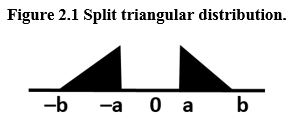
Figure 2.1 Split triangular distribution

Description for Figure 2.1

Figure illustrating the split triangular distribution. The distribution is null up to b. MathType@MTEF@5@5@+= feaagKart1ev2aqatCvAUfeBSjuyZL2yd9gzLbvyNv2CaerbuLwBLn hiov2DGi1BTfMBaeXatLxBI9gBaerbd9wDYLwzYbItLDharqqtubsr 4rNCHbGeaGqiFu0Je9sqqrpepC0xbbL8F4rqqrFgFv0dd9Wqpe0dd9 qqaqFeFr0xbbG8FaYPYRWFb9fi0lXxbvc9Ff0dfrpe0dXdHqps0=vr 0=vr0=fdbaqaaeGaciGaaiaabeqaamaabaabaaGcbaGaeyOeI0Iaam Oyaiaac6caaaa@3684@ Then, the values increase linearly from b MathType@MTEF@5@5@+= feaagKart1ev2aqatCvAUfeBSjuyZL2yd9gzLbvyNv2CaerbuLwBLn hiov2DGi1BTfMBaeXatLxBI9gBaerbd9wDYLwzYbItLDharqqtubsr 4rNCHbGeaGqiFu0Je9sqqrpepC0xbbL8F4rqqrFgFv0dd9Wqpe0dd9 qqaqFeFr0xbbG8FaYPYRWFb9fi0lXxbvc9Ff0dfrpe0dXdHqps0=vr 0=vr0=fdbaqaaeGaciGaaiaabeqaamaabaabaaGcbaGaeyOeI0Iaam Oyaiaac6caaaa@3684@  to a, MathType@MTEF@5@5@+= feaagKart1ev2aqatCvAUfeBSjuyZL2yd9gzLbvyNv2CaerbuLwBLn hiov2DGi1BTfMBaeXatLxBI9gBaerbd9wDYLwzYbItLDharqqtubsr 4rNCHbGeaGqiFu0Je9sqqrpepC0xbbL8F4rqqrFgFv0dd9Wqpe0dd9 qqaqFeFr0xbbG8FaYPYRWFb9fi0lXxbvc9Ff0dfrpe0dXdHqps0=vr 0=vr0=fdbaqaaeGaciGaaiaabeqaamaabaabaaGcbaGaeyOeI0Iaam yyaiaacYcaaaa@3681@ the distribution showing a triangular shape. Then the distribution is null. It starts again at a MathType@MTEF@5@5@+= feaagKart1ev2aqatCvAUfeBSjuyZL2yd9gzLbvyNv2CaerbuLwBLn hiov2DGi1BTfMBaeXatLxBI9gBaerbd9wDYLwzYbItLDharqqtubsr 4rNCHbGeaGqiFu0Je9sqqrpepC0xbbL8F4rqqrFgFv0dd9Wqpe0dd9 qqaqFeFr0xbbG8FaYPYRWFb9fi0lXxbvc9Ff0dfrpe0dXdHqps0=vr 0=vr0=fdbaqaaeGaciGaaiaabeqaamaabaabaaGcbaGaamyyaaaa@34E4@ and linearly decreases to b, MathType@MTEF@5@5@+= feaagKart1ev2aqatCvAUfeBSjuyZL2yd9gzLbvyNv2CaerbuLwBLn hiov2DGi1BTfMBaeXatLxBI9gBaerbd9wDYLwzYbItLDharqqtubsr 4rNCHbGeaGqiFu0Je9sqqrpepC0xbbL8F4rqqrFgFv0dd9Wqpe0dd9 qqaqFeFr0xbbG8FaYPYRWFb9fi0lXxbvc9Ff0dfrpe0dXdHqps0=vr 0=vr0=fdbaqaaeGaciGaaiaabeqaamaabaabaaGcbaGaamOyaiaacY caaaa@3595@ the distribution showing a second triangular shape. After, the distribution is null.
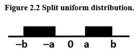
Figure 2.2 Split uniform distribution

Description for Figure 2.2

Figure illustrating the split uniform distribution. The distribution is non null only from b MathType@MTEF@5@5@+= feaagKart1ev2aqatCvAUfeBSjuyZL2yd9gzLbvyNv2CaerbuLwBLn hiov2DGi1BTfMBaeXatLxBI9gBaerbd9wDYLwzYbItLDharqqtubsr 4rNCHbGeaGqiFu0Je9sqqrpepC0xbbL8F4rqqrFgFv0dd9Wqpe0dd9 qqaqFeFr0xbbG8FaYPYRWFb9fi0lXxbvc9Ff0dfrpe0dXdHqps0=vr 0=vr0=fdbaqaaeGaciGaaiaabeqaamaabaabaaGcbaGaeyOeI0Iaam Oyaaaa@35D2@  to a MathType@MTEF@5@5@+= feaagKart1ev2aqatCvAUfeBSjuyZL2yd9gzLbvyNv2CaerbuLwBLn hiov2DGi1BTfMBaeXatLxBI9gBaerbd9wDYLwzYbItLDharqqtubsr 4rNCHbGeaGqiFu0Je9sqqrpepC0xbbL8F4rqqrFgFv0dd9Wqpe0dd9 qqaqFeFr0xbbG8FaYPYRWFb9fi0lXxbvc9Ff0dfrpe0dXdHqps0=vr 0=vr0=fdbaqaaeGaciGaaiaabeqaamaabaabaaGcbaGaeyOeI0Iaam yyaaaa@35D1@ and from a MathType@MTEF@5@5@+= feaagKart1ev2aqatCvAUfeBSjuyZL2yd9gzLbvyNv2CaerbuLwBLn hiov2DGi1BTfMBaeXatLxBI9gBaerbd9wDYLwzYbItLDharqqtubsr 4rNCHbGeaGqiFu0Je9sqqrpepC0xbbL8F4rqqrFgFv0dd9Wqpe0dd9 qqaqFeFr0xbbG8FaYPYRWFb9fi0lXxbvc9Ff0dfrpe0dXdHqps0=vr 0=vr0=fdbaqaaeGaciGaaiaabeqaamaabaabaaGcbaGaamyyaaaa@34E4@ to b, MathType@MTEF@5@5@+= feaagKart1ev2aqatCvAUfeBSjuyZL2yd9gzLbvyNv2CaerbuLwBLn hiov2DGi1BTfMBaeXatLxBI9gBaerbd9wDYLwzYbItLDharqqtubsr 4rNCHbGeaGqiFu0Je9sqqrpepC0xbbL8F4rqqrFgFv0dd9Wqpe0dd9 qqaqFeFr0xbbG8FaYPYRWFb9fi0lXxbvc9Ff0dfrpe0dXdHqps0=vr 0=vr0=fdbaqaaeGaciGaaiaabeqaamaabaabaaGcbaGaamOyaiaacY caaaa@3595@ showing two identical rectangular shapes.

There are ways to attenuate the cumulative impact of microdata perturbation on quality. Massell and Funk (2007) suggest to balance the random noises within cells for a primary table to limit their impact there. Other methods perturb microdata, but not always the same way, allowing some inconsistencies in results. Giessing (2011) proposes to multiply unit values x i MathType@MTEF@5@5@+= feaagKart1ev2aqatCvAUfeBSjuyZL2yd9gzLbvyNv2CaerbuLwBLn hiov2DGi1BTfMBaeXatLxBI9gBaerbd9wDYLwzYbItLDharqqtubsr 4rNCHbGeaGqiFu0Je9sqqrpepC0xbbL8F4rqqrFfFv0dd9Wqpe0dd9 qqaqFeFr0xbbG8FaYPYRWFb9fi0lXxbvc9Ff0dfrpe0dXdHqps0=vr 0=vr0=fdbaqaaeGaciGaaiaabeqaamaabaabaaGcbaGaamiEamaaBa aaleaacaWGPbaabeaaaaa@3611@ by w i = 1 ± | ε i | , MathType@MTEF@5@5@+= feaagKart1ev2aqatCvAUfeBSjuyZL2yd9gzLbvyNv2CaerbuLwBLn hiov2DGi1BTfMBaeXatLxBI9gBaerbd9wDYLwzYbItLDharqqtubsr 4rNCHbGeaGqiFu0Je9sqqrpepC0xbbL8F4rqqrFfFv0dd9Wqpe0dd9 qqaqFeFr0xbbG8FaYPYRWFb9fi0lXxbvc9Ff0dfrpe0dXdHqps0=vr 0=vr0=fdbaqaaeGaciGaaiaabeqaamaabaabaaGcbaGaam4DamaaBa aaleaacaWGPbaabeaakiabg2da9iaaigdacqGHXcqSdaabdaqaaiaa ykW7cqaH1oqzdaWgaaWcbaGaamyAaaqabaGccaaMc8oacaGLhWUaay jcSdGaaiilaaaa@437C@ for ε i MathType@MTEF@5@5@+= feaagKart1ev2aqatCvAUfeBSjuyZL2yd9gzLbvyNv2CaerbuLwBLn hiov2DGi1BTfMBaeXatLxBI9gBaerbd9wDYLwzYbItLDharqqtubsr 4rNCHbGeaGqiFu0Je9sqqrpepC0xbbL8F4rqqrFfFv0dd9Wqpe0dd9 qqaqFeFr0xbbG8FaYPYRWFb9fi0lXxbvc9Ff0dfrpe0dXdHqps0=vr 0=vr0=fdbaqaaeGaciGaaiaabeqaamaabaabaaGcbaGaeqyTdu2aaS baaSqaaiaadMgaaeqaaaaa@36BB@ i.i.d. N ( 0 , σ 0 2 ) , MathType@MTEF@5@5@+= feaagKart1ev2aqatCvAUfeBSjuyZL2yd9gzLbvyNv2CaerbuLwBLn hiov2DGi1BTfMBaeXatLxBI9gBaerbd9wDYLwzYbItLDharqqtubsr 4rNCHbGeaGqiFu0Je9sqqrpepC0xbbL8F4rqqrFfFv0dd9Wqpe0dd9 qqaqFeFr0xbbG8FaYPYRWFb9fi0lXxbvc9Ff0dfrpe0dXdHqps0=vr 0=vr0=fdbaqaaeGaciGaaiaabeqaamaabaabaaGcbiqaaGYdcaqGob WaaeWaaeaacaaIWaGaaiilaiabeo8aZnaaDaaaleaacaaIWaaabaGa aGOmaaaaaOGaayjkaiaawMcaaiaacYcaaaa@3C18@ except in sensitive cells, where the largest value gets multiplied by w i = 1 ± ( μ 0 + | ε i | ) . MathType@MTEF@5@5@+= feaagKart1ev2aqatCvAUfeBSjuyZL2yd9gzLbvyNv2CaerbuLwBLn hiov2DGi1BTfMBaeXatLxBI9gBaerbd9wDYLwzYbItLDharqqtubsr 4rNCHbGeaGqiFu0Je9sqqrpepC0xbbL8F4rqqrFfFv0dd9Wqpe0dd9 qqaqFeFr0xbbG8FaYPYRWFb9fi0lXxbvc9Ff0dfrpe0dXdHqps0=vr 0=vr0=fdbaqaaeGaciGaaiaabeqaamaabaabaaGcbaGaam4DamaaBa aaleaacaWGPbaabeaakiabg2da9iaaigdacqGHXcqSdaqadaqaaiab eY7aTnaaBaaaleaacaaIWaaabeaakiabgUcaRmaaemaabaGaaGPaVl abew7aLnaaBaaaleaacaWGPbaabeaakiaaykW7aiaawEa7caGLiWoa caaMc8oacaGLOaGaayzkaaGaaiOlaaaa@4A1A@ The value μ 0 MathType@MTEF@5@5@+= feaagKart1ev2aqatCvAUfeBSjuyZL2yd9gzLbvyNv2CaerbuLwBLn hiov2DGi1BTfMBaeXatLxBI9gBaerbd9wDYLwzYbItLDharqqtubsr 4rNCHbGeaGqiFu0Je9sqqrpepC0xbbL8F4rqqrFfFv0dd9Wqpe0dd9 qqaqFeFr0xbbG8FaYPYRWFb9fi0lXxbvc9Ff0dfrpe0dXdHqps0=vr 0=vr0=fdbaqaaeGaciGaaiaabeqaamaabaabaaGcbaGaeqiVd02aaS baaSqaaiaaicdaaeqaaaaa@3696@ is chosen to give an appropriate level of protection for sensitive cells, allowing a lower value of σ 0 2 MathType@MTEF@5@5@+= feaagKart1ev2aqatCvAUfeBSjuyZL2yd9gzLbvyNv2CaerbuLwBLn hiov2DGi1BTfMBaeXatLxBI9gBaerbd9wDYLwzYbItLDharqqtubsr 4rNCHbGeaGqiFu0Je9sqqrpepC0xbbL8F4rqqrFfFv0dd9Wqpe0dd9 qqaqFeFr0xbbG8FaYPYRWFb9fi0lXxbvc9Ff0dfrpe0dXdHqps0=vr 0=vr0=fdbaqaaeGaciGaaiaabeqaamaabaabaaGcbaaeaaaaaaaaa8 qacqaHdpWCpaWaa0baaSqaa8qacaaIWaaapaqaa8qacaaIYaaaaaaa @37BE@ to be used overall. But if σ 0 2 MathType@MTEF@5@5@+= feaagKart1ev2aqatCvAUfeBSjuyZL2yd9gzLbvyNv2CaerbuLwBLn hiov2DGi1BTfMBaeXatLxBI9gBaerbd9wDYLwzYbItLDharqqtubsr 4rNCHbGeaGqiFu0Je9sqqrpepC0xbbL8F4rqqrFfFv0dd9Wqpe0dd9 qqaqFeFr0xbbG8FaYPYRWFb9fi0lXxbvc9Ff0dfrpe0dXdHqps0=vr 0=vr0=fdbaqaaeGaciGaaiaabeqaamaabaabaaGcbaaeaaaaaaaaa8 qacqaHdpWCpaWaa0baaSqaa8qacaaIWaaapaqaa8qacaaIYaaaaaaa @37BE@ is too low the method may not sufficiently protect against disclosure by differencing. The Australian Bureau of Statistics’ Top Contributors Method (TCM), developed for its TableBuilder remote access application, consists of perturbing the largest respondents in each cell in a semi-consistent way, i.e., where parts of their noise is applied consistently (Thompson, Broadfoot and Elazar 2013). The LPM uses some of the same concepts but, as will be explained, protects more against differencing.

Other commonly used strategies such as rounding, (sub-)sampling and swapping units, say between neighbouring areas, are better suited for the protection of frequency tables.


Date modified: