
Economic and Social Reports
Survey framing and mode effects in life satisfaction responses on Canadian social surveys
DOI: https://doi.org/10.25318/36280001202300100003-eng
Skip to text
Text begins
Abstract
Quality of life and well-being research often involves survey content that is subjective in nature, for example, questions pertaining to life satisfaction. Two phenomena impacting responses to self-reported life satisfaction are studied across a range of social surveys: the framing effect, where a respondent’s answer is influenced by the theme of the survey or its content; and the mode effect, where a respondent’s answer is influenced by the method in which survey data are collected (with an interviewer, through an online collection portal, etc.). The impact of these effects on life satisfaction responses is measured across three Statistics Canada survey series: the General Social Survey (GSS), the Canadian Community Health Survey (CCHS) and the Canadian Social Survey. The GSS uses a different theme each year that fits into one of four categories and serves as the main source of variation in survey theme. Significant framing effects are observed for each theme of the GSS relative to the CCHS, and they explain a large portion of between-year variations in average self-reported life satisfaction. A mode effect is also observed for electronic questionnaire collection relative to computer-assisted telephone interviews. Differences in life satisfaction scores across a variety of demographic concepts are also presented.
Keywords: Quality of life, well-being, life satisfaction, framing effect, mode effect, social survey
Authors
David Wavrock and Grant Schellenberg are with the Social Analysis and Modelling Division, Analytical Studies and Modelling Branch, Statistics Canada. Cilanne Boulet is with the Social Statistics Methods Division, Modern Statistical Methods and Data Science Branch, Statistics Canada.
Introduction
The objective of this paper is to document the effect of survey collection and survey content on Canadians’ self-reported satisfaction with their lives. Two phenomena are studied. The first is the survey framing effect, whereby a survey respondent’s answer to a question is influenced by the content or theme of the survey they are completing. The second is the survey mode effect, whereby a respondent’s answer to a question is influenced by how they complete the survey, for example, by completing a questionnaire online by themselves or by completing a telephone interview with a Statistics Canada representative.
Survey framing and survey mode effects (henceforth, framing and mode effects) have the potential to influence all survey responses, although their potential impact on subjective questions is of particular consideration. With framing effects, an individual’s line of thought may be “primed” by the preceding sequence of survey questions, whereas with mode effects, an individual may be more or less willing to accurately report how they feel about a topic if they think their response could elicit a negative response from an interviewer (i.e., social desirability bias) (Atkeson, Adams and Alvarez 2014; Tourangeau and Yan 2007). Prior research at Statistics Canada has found evidence of the former phenomenon on life satisfaction content on some social surveys (Bonikowska et al. 2014), but this research was conducted before the introduction of electronic questionnaire (EQ) collection and, hence, does not include the impact of survey mode on responses.
It is worthwhile to revisit framing and mode effects given the changing context in which household surveys are being fielded. A shift towards online data collection has been underway at Statistics Canada for many years now. Most household responses to the 2016 and 2021 censuses of population were provided online. Likewise, online data collection for the General Social Survey (GSS) was first introduced in 2013 and has accounted for a growing share of responses since then. The shift to online collection was accelerated in 2020 by the COVID-19 pandemic and Statistics Canada’s organizational response to it. Looking ahead, the shift to online survey collection will continue, and therefore, an examination of the impact that this shift will have is warranted.
Framing and mode effects also warrant consideration given the range of purposes for which survey data are being used. Survey data are an important source of indicators that are included in the indicator framework initiatives being implemented at all levels of government. The Organisation for Economic Co‑operation and Development’s (OECD) Better Life Initiative is an example of this type of initiative at the international level, while the Quality of Life Framework, the Gender Results Framework and the Social Inclusion Framework are examples at the national level in Canada (Sanmartin et al. 2021). Changes in indicator levels from year to year are intended to signal developments or trends deemed to be positive or negative. Results confounded by framing or mode effects may provide misleading information, and their potential impacts warrant estimation. In addition, Statistics Canada is fielding new survey initiatives designed to gather information on social issues using smaller samples and shorter processing times than traditional household surveys. The Canadian Social Survey (CSS) is one example. Given the focus of these surveys on social topics, framing and mode effects are a consideration.
This study examines responses to a standard question about satisfaction with life overall collected in more than a dozen years of the GSS, three years of the Canadian Community Health Survey (CCHS) and three waves of the CSS. Of central interest are differences in the levels and distributions of life satisfaction responses observed across survey modes (via telephone, in person or online) and survey themes, net of survey respondents’ socioeconomic characteristics. Life satisfaction is selected as the outcome of interest in this study because it is a subjective measure that continues to be the focus of a large and growing body of academic and public policy research. Moreover, it is the OECD’s recommended measure of subjective well-being and is a headline indicator in Canada’s Quality of Life Framework (OECD 2013).
Data and methods
This study is based on data from three Statistics Canada surveys: the GSS, the CCHS and the CSS.
Established in 1985, the GSS is an annual cross-sectional survey that collects data on social trends and issues to monitor changes in the living conditions and well-being of Canadians, and to provide information on specific issues relevant to social policy. Each year, information is collected on a specific theme, such as time use, victimization or social identity, with these themes repeated at approximately five-year intervals. The target population of the GSS is non-institutionalized persons 15 years of age or older residing in Canada’s 10 provinces.
The CCHS is an annual cross-sectional survey that collects information related to the health status, health care utilization and determinants of health among the Canadian population and has been in collection since 2001. The CCHS provides crucial information on health outcomes at the national, provincial and subprovincial levels and is an important data source for health surveillance and population health research in Canada. The target population of the CCHS is non-institutionalized persons 12 years of age or older in the Canadian provinces.
The CSS is one of Statistics Canada’s newest data collection projects, and it aims to understand social issues more rapidly by conducting surveys on different topics every three months. Starting in 2021, the CSS has collected information on social topics such as health and well-being, impacts of COVID-19 on the public, activities and time use, and emergency preparedness. Each wave of the survey is given a different theme, but unlike the GSS, these themes are not necessarily repeated at regular intervals. The target population of the CSS is non-institutionalized persons 15 years of age or older in the Canadian provinces.
Within these three survey streams, the focus of the present study is on content regarding self-reported satisfaction with life as a whole. A standard question on life satisfaction has been included on most GSS questionnaires since 2003, on all CCHS questionnaires since 2009 and on all CSS questionnaires since the launch of the survey in 2021. Specifically, respondents are asked the following:
Earlier iterations of the GSS, specifically those in 2003, 2005 and 2006, asked a series of questions related to satisfaction with various domains of life. In these surveys, respondents were asked the following:
I am going to ask you to rate certain areas of your life. Please rate your feelings about them, using a scale of 1 to 10 where 1 means “Very dissatisfied” and 10 means “Very satisfied.”
What about…
… your health?
… your job or main activity?
… the way you spend your other time?
… your finances?
Using the same scale, how do you feel about your life as a whole right now?
Although the wording and placementNote of the question in the survey changed slightly in these early iterations of the GSS, the question, “How do you feel about your life as a whole right now?” remained constant. Before 2011, GSS respondents answered the life satisfaction question using a response scale ranging from 1 to 10, while from 2011 onwards, they answered using a response scale ranging from 0 to 10. On each survey since 2011, less than 1% of respondents provided a 0 response, and for this study, these were combined with responses of 1 to make the response scale consistent across all surveys.
From 2003 to 2019, three iterations of the GSS were fielded in each of four thematic areas: time use, victimization, social identity and family (see Table 1). From 2017 to 2019, three iterations of the CCHS were fielded and are treated as a fifth thematic area in this study. Together, these five themes provide the basis for estimating the impacts of survey framing effects on life satisfaction responses. The analysis of survey mode effects, including computer-assisted telephone interviewing (CATI), computer-assisted personal interviewing (CAPI) and EQs completed by respondents themselves, was run separately for GSS and CCHS respondents. Two iterations of the GSS that were fielded in 2018—one on caregiving and care receiving and one on giving, volunteering and participation—were also included in the analysis of mode effects. Additionally, three iterations of the CSS fielded in 2021 were included in a supplementary analysis of mode effects. Aside from these supplementary CSS results, the data for this study were all collected before the onset of the COVID-19 pandemic, thereby removing any confounding effects of that event on the estimates of framing and mode effects.Note
| Survey | Survey year | Survey theme | Theme group | Sample size |
|---|---|---|---|---|
| GSS, Cycle 17 | 2003 | Social Engagement | A - Social identity | 24,951 |
| GSS, Cycle 19 | 2005 | Time Use | C - Time use | 19,597 |
| GSS, Cycle 20 | 2006 | Family Transitions | D - Family | 23,608 |
| GSS, Cycle 22 | 2008 | Social Networks | A - Social identity | 20,401 |
| GSS, Cycle 23 | 2009 | Victimization | B - Victimization | 19,422 |
| GSS, Cycle 24 | 2010 | Time Use | C - Time use | 15,390 |
| GSS, Cycle 25 | 2011 | Family | D - Family | 22,435 |
| GSS, Cycle 27 | 2013 | Social Identity | A - Social identity | 27,695 |
| GSS, Cycle 28 | 2014 | Victimization | B - Victimization | 33,127 |
| GSS, Cycle 29 | 2015 | Time Use | C - Time use | 17,390 |
| GSS, Cycle 31 | 2017 | Family | D - Family | 20,602 |
| GSS, Cycle 32 | 2018 | Caregiving and Care Receiving | n/a | 20,258 |
| GSS, Cycle 33 | 2018 | Giving, Volunteering and Participating | n/a | 16,149 |
| GSS, Cycle 34 | 2019 | Canadians' SafetyTable 1 Note 1 | B - Victimization | 20,454 |
| CCHS | 2017 | Health | E - Health | 54,660 |
| CCHS | 2018 | Health | E - Health | 52,053 |
| CCHS | 2019 | Health | E - Health | 63,007 |
| CSS, Wave 1 | 2021 | COVID-19 and Well-being | n/a | 10,602 |
| CSS, Wave 2 | 2021 | Well-being, Activities and Perception of Time | n/a | 9,781 |
| CSS, Wave 3 | 2021 | Well-being, Unpaid Work and Family Time | n/a | 9,951 |
Sources: Statistics Canada, General Social Survey, 2003, 2005, 2006, 2008, 2009, 2010, 2011, 2013, 2014, 2015, 2017, 2018 (cycles 32 and 33) and 2019; Canadian Community Health Survey, 2017, 2018 and 2019; and Canadian Social Survey, 2021 (waves 1, 2 and 3). |
||||
Data from the surveys above were pooled together in an analytical file composed of a consistent set of life satisfaction and socioeconomic variables. These include age, sex, educational attainment, household income, marital status, household size, presence of children, immigrant status, province of residence, rural or urban residence, and self-assessed general health. CCHS respondents aged 12 to 14 were dropped from the file for consistency with the GSS and CSS. Finally, information on survey year, theme and mode was appended to each respondent. Overall, the final analytical file comprises over 470,000 respondents from 20 surveys spanning 18 years.
Framing and mode effects are examined both in terms of overall level differences in average life satisfaction and in terms of distributional differences across age groups. Ordinary least squares (OLS) regression models are used for the multivariate analysis, with life satisfaction responses regressed against theme and mode variables, as well as the socioeconomic characteristics listed above. The latter variables take into account any differences in the compositional characteristics of respondents across surveys. The analysis was also run using ordinal logit and probit models. These yielded results similar to those from the OLS models, and only the latter are given below for ease of presentation. All results were calculated using survey weights from the respective surveys.
Results
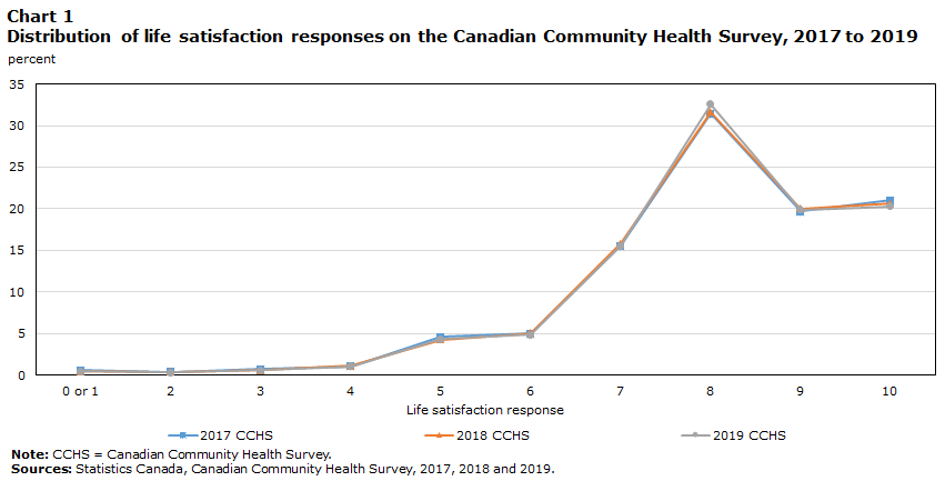
Starting with a look at life satisfaction responses across surveys, Table 2 presents both average life satisfaction and the distributions of life satisfaction responses on the 1 to 10 scale. The latter information is presented graphically in charts 1 to 4.
| Life satisfaction response | 2003 GSS | 2005 GSS | 2006 GSS | 2008 GSS | 2009 GSS | 2010 GSS | 2011 GSS | 2013 GSS | 2014 GSS | 2015 GSS | 2017 GSS |
|---|---|---|---|---|---|---|---|---|---|---|---|
| percent | |||||||||||
| 0 or 1 | 0.7 | 0.6 | 0.7 | 0.6 | 0.5 | 1.2 | 0.7 | 0.8 | 0.4 | 1.2 | 0.4 |
| 2 | 0.5 | 0.4 | 0.4 | 0.7 | 0.3 | 0.6 | 0.4 | 0.7 | 0.3 | 0.7 | 0.3 |
| 3 | 0.8 | 0.9 | 0.9 | 1.0 | 0.6 | 1.2 | 0.5 | 1.3 | 0.4 | 1.3 | 0.6 |
| 4 | 1.1 | 1.5 | 1.4 | 1.4 | 1.0 | 2.0 | 1.0 | 1.6 | 0.9 | 2.1 | 1.2 |
| 5 | 5.7 | 6.2 | 4.8 | 6.4 | 4.3 | 7.5 | 4.5 | 5.8 | 3.3 | 7.7 | 4.7 |
| 6 | 5.8 | 8.0 | 5.7 | 5.7 | 3.5 | 8.0 | 5.1 | 5.6 | 3.8 | 8.1 | 5.1 |
| 7 | 17.5 | 19.6 | 16.4 | 16.8 | 12.6 | 19.2 | 15.2 | 16.6 | 12.9 | 20.2 | 16.2 |
| 8 | 31.6 | 31.6 | 31.1 | 31.0 | 29.7 | 31.1 | 31.1 | 30.3 | 29.6 | 28.9 | 30.3 |
| 9 | 19.3 | 17.2 | 20.5 | 15.9 | 17.7 | 14.7 | 18.9 | 17.3 | 19.4 | 12.8 | 18.8 |
| 10 | 17.0 | 14.0 | 18.2 | 20.6 | 29.7 | 14.6 | 22.6 | 19.8 | 29.0 | 17.0 | 22.4 |
| average on life satisfaction response scale | |||||||||||
| Average | 7.9 | 7.7 | 8.0 | 7.9 | 8.3 | 7.6 | 8.1 | 7.9 | 8.4 | 7.6 | 8.1 |
| Sources: Statistics Canada, General Social Survey, 2003, 2005, 2006, 2008, 2009, 2010, 2011, 2013, 2014, 2015, 2017, 2018 (cycles 32 and 33) and 2019; Canadian Community Health Survey, 2017, 2018 and 2019; and Canadian Social Survey, 2021 (waves 1, 2 and 3). | |||||||||||
| Life satisfaction response | 2018 GSS, Cycle 32 |
2018 GSS, Cycle 33 |
2019 GSS | 2017 CCHS | 2018 CCHS | 2019 CCHS | CSS Wave 1 |
CSS Wave 2 |
CSS Wave 3 |
|---|---|---|---|---|---|---|---|---|---|
| percent | |||||||||
| 0 or 1 | 1.3 | 1.4 | 1.0 | 0.6 | 0.4 | 0.5 | 2.4 | 1.4 | 1.8 |
| 2 | 1.1 | 1.1 | 0.8 | 0.4 | 0.4 | 0.3 | 2.0 | 1.2 | 1.6 |
| 3 | 1.9 | 1.5 | 1.3 | 0.8 | 0.6 | 0.6 | 4.4 | 2.4 | 2.8 |
| 4 | 2.6 | 1.6 | 1.8 | 1.1 | 1.1 | 1.0 | 5.2 | 3.4 | 3.3 |
| 5 | 8.3 | 7.6 | 6.5 | 4.6 | 4.3 | 4.3 | 13.4 | 8.9 | 9.6 |
| 6 | 8.1 | 7.1 | 6.0 | 5.0 | 5.1 | 4.9 | 10.3 | 8.4 | 9.5 |
| 7 | 19.0 | 18.6 | 15.6 | 15.5 | 15.8 | 15.5 | 20.4 | 20.2 | 19.2 |
| 8 | 27.4 | 28.4 | 26.1 | 31.4 | 31.6 | 32.6 | 21.8 | 25.5 | 25.2 |
| 9 | 13.4 | 14.3 | 16.0 | 19.7 | 20.1 | 19.9 | 9.5 | 13.7 | 13.1 |
| 10 | 16.9 | 18.6 | 24.8 | 21.0 | 20.6 | 20.3 | 10.6 | 14.9 | 13.8 |
| average on life satisfaction response scale | |||||||||
| Average | 7.52 | 7.66 | 7.92 | 8.08 | 8.10 | 8.10 | 6.78 | 7.37 | 7.24 |
|
Notes: GSS = General Social Survey; CCHS = Canadian Community Health Survey; CSS = Canadian Social Survey. Sources: Statistics Canada, General Social Survey, 2003, 2005, 2006, 2008, 2009, 2010, 2011, 2013, 2014, 2015, 2017, 2018 (cycles 32 and 33) and 2019; Canadian Community Health Survey, 2017, 2018 and 2019; and Canadian Social Survey, 2021 (waves 1, 2 and 3). |
|||||||||
Average life satisfaction varies considerably across iterations of the GSS, ranging from 7.52 in 2018 (Cycle 32, Caregiving and Care Receiving) to 8.37 in 2014. Year-to-year differences are also substantial in some instances, with average life satisfaction 0.78 points lower in 2015 than in 2014 and 0.51 points higher in 2011 than in 2010. A closer look at the underlying distributions shows that this variability in averages likely reflects the shares of respondents reporting life satisfaction of 7, 8, 9 or 10, which together comprise the vast majority of respondents. In contrast to the GSS, the CCHS yields very stable estimates of life satisfaction. From 2017 to 2019, average life satisfaction differed by 0.02 points on the CCHS, compared with a maximum difference of 0.58 on the GSS over the same period.
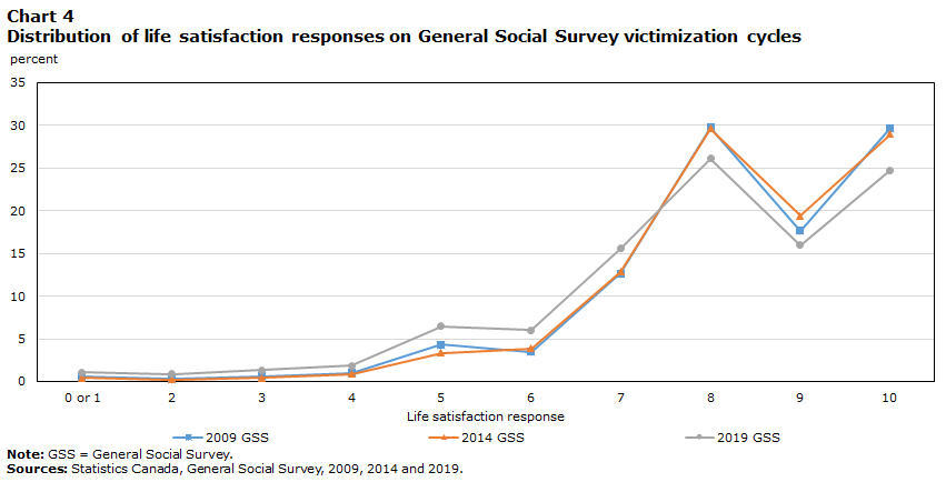
The consistency of life satisfaction responses on the CCHS is visually evident in Chart 1, since the distributions of responses are nearly indistinguishable across years. Distributions are also highly consistent across GSS iterations within thematic areas, particularly social identity and family (not shown)—differences of 2 to 3 percentage points on the 9 and 10 response categories are the largest observed. Life satisfaction distributions vary slightly more across GSS time use cycles, although again the largest difference observed is about 4 percentage points.Note Finally, the life satisfaction distributions on the 2009 and 2014 GSS – Victimization cycles closely overlap, but the 2019 cycle does not. A shift in content on the 2019 GSS likely contributes to this difference, as topics pertaining to Canadians’ safety were covered that year, in contrast to the focus on victimization in 2009 and 2014. Furthermore, both CATI and EQ collection were used in 2019, while only CATI was used in 2009 and 2014. This contributes to the differences in life satisfaction responses across these years, as discussed in more detail below. Overall, the GSS generally yields quite consistent life satisfaction distributions within survey themes. In contrast, larger differences across survey themes are observed. For example, the share of respondents rating their life satisfaction as 10 ranges from around 15% in time use cycles, to around 20% in family and social identity cycles, to 25% to 30% in victimization cycles.
Data table for Chart 1
| Life satisfaction response | 2017 CCHS | 2018 CCHS | 2019 CCHS |
|---|---|---|---|
| percent | |||
| 0 or 1 | 0.56 | 0.44 | 0.47 |
| 2 | 0.37 | 0.36 | 0.35 |
| 3 | 0.75 | 0.58 | 0.62 |
| 4 | 1.09 | 1.13 | 1.04 |
| 5 | 4.57 | 4.27 | 4.34 |
| 6 | 5.00 | 5.09 | 4.88 |
| 7 | 15.53 | 15.81 | 15.54 |
| 8 | 31.45 | 31.63 | 32.58 |
| 9 | 19.67 | 20.06 | 19.91 |
| 10 | 21.01 | 20.62 | 20.28 |
|
Note: CCHS = Canadian Community Health Survey. Sources: Statistics Canada, Canadian Community Health Survey, 2017, 2018 and 2019. |
|||

Data table for Chart 2
| Life satisfaction response | 2003 GSS | 2008 GSS | 2013 GSS |
|---|---|---|---|
| percent | |||
| 0 or 1 | 0.68 | 0.59 | 0.84 |
| 2 | 0.52 | 0.67 | 0.69 |
| 3 | 0.83 | 1.02 | 1.29 |
| 4 | 1.14 | 1.40 | 1.65 |
| 5 | 5.72 | 6.36 | 5.84 |
| 6 | 5.78 | 5.69 | 5.61 |
| 7 | 17.54 | 16.82 | 16.58 |
| 8 | 31.56 | 30.99 | 30.32 |
| 9 | 19.27 | 15.90 | 17.34 |
| 10 | 16.95 | 20.56 | 19.83 |
|
Note: GSS = General Social Survey. Sources: Statistics Canada, General Social Survey, 2003, 2008 and 2013. |
|||

Data table for Chart 3
| Life satisfaction response | 2005 GSS | 2010 GSS | 2015 GSS |
|---|---|---|---|
| percent | |||
| 0 or 1 | 0.62 | 1.17 | 1.23 |
| 2 | 0.40 | 0.62 | 0.74 |
| 3 | 0.94 | 1.20 | 1.28 |
| 4 | 1.54 | 2.02 | 2.12 |
| 5 | 6.19 | 7.45 | 7.70 |
| 6 | 7.99 | 7.99 | 8.14 |
| 7 | 19.56 | 19.19 | 20.17 |
| 8 | 31.60 | 31.12 | 28.87 |
| 9 | 17.18 | 14.66 | 12.79 |
| 10 | 13.97 | 14.57 | 16.95 |
|
Note: GSS = General Social Survey. Sources: Statistics Canada, General Social Survey, 2005, 2010 and 2015. |
|||
Data table for Chart 4
| Life satisfaction response | 2009 GSS | 2014 GSS | 2019 GSS |
|---|---|---|---|
| percent | |||
| 0 or 1 | 0.55 | 0.39 | 1.05 |
| 2 | 0.26 | 0.25 | 0.85 |
| 3 | 0.60 | 0.41 | 1.34 |
| 4 | 1.02 | 0.90 | 1.85 |
| 5 | 4.34 | 3.34 | 6.47 |
| 6 | 3.49 | 3.84 | 6.03 |
| 7 | 12.64 | 12.85 | 15.56 |
| 8 | 29.75 | 29.64 | 26.11 |
| 9 | 17.68 | 19.39 | 15.99 |
| 10 | 29.67 | 28.98 | 24.76 |
|
Note: GSS = General Social Survey. Sources: Statistics Canada, General Social Survey, 2009, 2014 and 2019. |
|||
Regression coefficients in Table 3 show that these differences between surveys are not explained by variations in the demographic composition of each survey’s sample. The 2019 CCHS was used as a reference group and socioeconomic characteristics (see Table 6) were taken into account to estimate coefficients for each survey. Life satisfaction on each GSS was significantly different from the 2019 CCHS, with responses generally lowest on GSS time use cycles and generally highest on GSS victimization cycles. The 2019 GSS – Canadians’ Safety is one notable exception. The multivariate results confirm that life satisfaction responses on the 2017 and 2018 CCHS did not differ significantly from those on the 2019 CCHS.
| Coefficient | Standard error | |
|---|---|---|
| Survey and theme | ||
| 2005 GSS, time use | -0.223Note *** | 0.0141 |
| 2010 GSS, time use | -0.358Note *** | 0.0138 |
| 2015 GSS, time use | -0.371Note *** | 0.0130 |
| 2002 GSS, social identity | -0.150Note *** | 0.0140 |
| 2008 GSS, social identity | -0.064Note *** | 0.0137 |
| 2013 GSS, social identity | -0.213Note *** | 0.0136 |
| 2006 GSS, family | -0.023 | 0.0139 |
| 2011 GSS, family | 0.078Note *** | 0.0136 |
| 2017 GSS, family | 0.066Note *** | 0.0129 |
| 2009 GSS, victimization | 0.207Note *** | 0.0137 |
| 2014 GSS, victimization | 0.285Note *** | 0.0143 |
| 2019 GSS, victimization | -0.085Note *** | 0.0129 |
| 2018 GSS, Cycle 32 | -0.499Note *** | 0.0130 |
| 2018 GSS, Cycle 33 | -0.302Note *** | 0.0131 |
| 2017 CCHS, health | 0.003 | 0.0130 |
| 2018 CCHS, health | 0.015 | 0.0130 |
| 2019 CCHS, health (ref.) | ... | ... |
| Adjusted R-square | 0.219 | Note ...: not applicable |
|
... not applicable * significantly different from reference category (p < 0.05) ** significantly different from reference category (p < 0.01)
Sources: Statistics Canada, General Social Survey and Canadian Community Health Survey, various years. |
||
Survey framing effects
To consolidate the analysis of survey framing effects, a survey theme variable was constructed for a series of regression models, along with a survey mode variable and socioeconomic variables. Results from these models are presented in Table 4. Column 1 confirms that survey themes have statistically significant impacts on life satisfaction responses. GSS victimization cycles yield an estimate of average life satisfaction that is 0.10 points higher than that from the CCHS. (If the 2019 GSS – Canadians’ Safety is excluded from that theme, the coefficient increases to 0.24 points.) The GSS time use cycles yield an average life satisfaction estimate that is 0.34 points lower than that observed on the CCHS. Life satisfaction estimates are also relatively low in social identity cycles, 0.15 points lower than the CCHS.
| Model | Column 1 Framing effects (GSS and CCHS) |
Column 2 Mode effects (GSS only) |
Column 3 Mode effects (CCHS only) |
Column 4 Mode effects (CSS only) |
Column 5 Framing and mode effects (GSS and CCHS) |
|---|---|---|---|---|---|
| Survey theme | |||||
| Social identity | |||||
| Coefficient | -0.1536Note *** | Note ...: not applicable | Note ...: not applicable | Note ...: not applicable | -0.1145Note *** |
| Standard error | 0.0077 | Note ...: not applicable | Note ...: not applicable | Note ...: not applicable | 0.0083 |
| Victimization | |||||
| Coefficient | 0.1024Note *** | Note ...: not applicable | Note ...: not applicable | Note ...: not applicable | 0.2121Note *** |
| Standard error | 0.0075 | Note ...: not applicable | Note ...: not applicable | Note ...: not applicable | 0.0085 |
| Time use | |||||
| Coefficient | -0.3373Note *** | Note ...: not applicable | Note ...: not applicable | Note ...: not applicable | -0.3381Note *** |
| Standard error | 0.0075 | Note ...: not applicable | Note ...: not applicable | Note ...: not applicable | 0.0081 |
| Family | |||||
| Coefficient | 0.0327Note *** | Note ...: not applicable | Note ...: not applicable | Note ...: not applicable | 0.0185Note * |
| Standard error | 0.0075 | Note ...: not applicable | Note ...: not applicable | Note ...: not applicable | 0.0080 |
| Health (ref.) | Note ...: not applicable | Note ...: not applicable | Note ...: not applicable | Note ...: not applicable | |
| Collection mode | |||||
| CATI (ref.) | Note ...: not applicable | Note ...: not applicable | Note ...: not applicable | Note ...: not applicable | Note ...: not applicable |
| EQ | |||||
| Coefficient | Note ...: not applicable | -0.4564Note *** | Note ...: not applicable | -0.6148Note *** | -0.4654Note *** |
| Standard error | Note ...: not applicable | 0.0083 | Note ...: not applicable | 0.0273 | 0.0097 |
| CAPI | |||||
| Coefficient | Note ...: not applicable | Note ...: not applicable | -0.0785Note *** | Note ...: not applicable | -0.0662Note *** |
| Standard error | Note ...: not applicable | Note ...: not applicable | 0.0080 | Note ...: not applicable | 0.0118 |
| Adjusted R-square | 0.2082 | 0.2019 | 0.2746 | 0.2321 | 0.2131 |
| number | |||||
| Number of observations | 376,045 | 248,966 | 161,116 | 29,835 | 376,043 |
... not applicable
Sources: Statistics Canada, General Social Survey, Canadian Community Health Survey and Canadian Social Survey, various years. |
|||||
From this, it appears that framing effects account for a significant portion of year-over-year variations in life satisfaction observed on the GSS. The 0.78-point decline in life satisfaction observed from 2014 to 2015 coincides with a change in theme from victimization, the theme with the most positive framing effect, to time use, the theme with the most negative framing effect. The coefficients above suggest that this accounts for approximately 0.44 points of the 0.78-point difference (56% of the difference) in life satisfaction between those years.Note Similarly, the 0.51-point increase in life satisfaction observed between the 2010 and 2011 GSS coincided with a change from the time use to the family theme and an estimated framing effect of 0.37 points (73% of the difference).
GSS cycles on time use ask respondents about their perceptions and use of time before asking them about life satisfaction. Questions about “time crunch” (e.g., “Do you feel trapped in a daily routine?”) and unpaid labour (e.g., housework and childcare) appear to prime respondents, yielding lower life satisfaction responses than would otherwise result. Bonikowska et al. (2014) found that this effect is strongest among GSS respondents working more than 40 hours per week. In the GSS cycles on victimization, the life satisfaction question is located fairly late in the survey (module 13 of 16), after numerous questions regarding personal experiences with crime incidence, victimization and abuse. Responses to the life satisfaction question in the survey may be higher because most respondents recall that nothing “bad” happened to them during the reference period (Bonikowska et al. 2014).
Survey mode effects
Before 2013, all responses to the GSS were collected via CATI. GSS data collection using EQ was first introduced in 2013 and subsequently used in 2015, 2018 and 2019. The 2017 to 2019 CCHS used CATI as the main collection mode, as well as some CAPI.
Table 5 presents average life satisfaction by collection mode for each survey where multiple modes were used. On average, GSS and CSS EQ respondents reported lower life satisfaction than CATI respondents, with the difference ranging from 0.36 to 0.63 points. On the CCHS, life satisfaction was higher among CATI than CAPI respondents, with the difference ranging from 0.21 and 0.23 points.
| CATI | EQ | CAPI | Difference vis-à-vis CATI | |
|---|---|---|---|---|
| average on life satisfaction response scale | ||||
| 2013 GSS | 8.01 | 7.58 | Note ...: not applicable | -0.42 |
| 2015 GSS | 7.63 | 7.12 | Note ...: not applicable | -0.51 |
| 2018 GSS, Cycle 32 | 7.80 | 7.30 | Note ...: not applicable | -0.50 |
| 2018 GSS, Cycle 33 | 7.90 | 7.48 | Note ...: not applicable | -0.42 |
| 2019 GSS | 8.16 | 7.80 | Note ...: not applicable | -0.36 |
| 2017 CCHS | 8.13 | Note ...: not applicable | 7.93 | -0.21 |
| 2018 CCHS | 8.15 | Note ...: not applicable | 7.92 | -0.23 |
| 2019 CCHS | 8.16 | Note ...: not applicable | 7.93 | -0.23 |
| CSS, Wave 1 | 7.28 | 6.65 | Note ...: not applicable | -0.63 |
| CSS, Wave 2 | 7.73 | 7.29 | Note ...: not applicable | -0.44 |
| CSS, Wave 3 | 7.70 | 7.11 | Note ...: not applicable | -0.59 |
|
... not applicable Notes: GSS = General Social Survey; CCHS = Canadian Community Health Survey; CSS = Canadian Social Survey; CATI = computer-assisted telephone interviewing; EQ = electronic questionnaire; CAPI = computer-assisted personal interviewing. Sources: Statistics Canada, General Social Survey, Canadian Community Health Survey and Canadian Social Survey, various years. |
||||
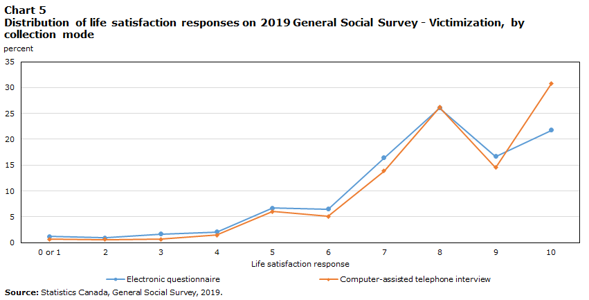
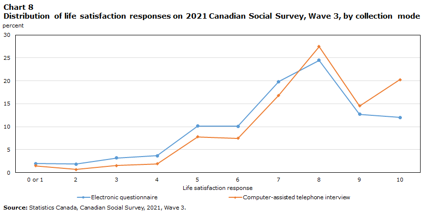
The distributions of life satisfaction responses provided by GSS and CSS respondents who completed their questionnaire via EQ or CATI are shown in charts 5 through 8 (also, see Appendix Tables 1-1, 1-2 and 1-3). On the 2018 and 2019 GSS iterations, the shares of respondents rating their life satisfaction as 10 were 6 to 9 percentage points lower among EQ respondents than CATI respondents. Conversely, the shares of EQ respondents reporting their life satisfaction as 5, 6 or 7 were 4 to 7 percentage points higher than CATI respondents. The differences were larger on Wave 3 of the 2021 CSS, with the distribution of life satisfaction responses of EQ respondents positioned to the left of (i.e., lower than) the distribution of CATI respondents.
Data table for Chart 5
| Life satisfaction response | Electronic questionnaire | Computer-assisted telephone interview |
|---|---|---|
| percent | ||
| 0 or 1 | 1.22 | 0.70 |
| 2 | 0.96 | 0.62 |
| 3 | 1.67 | 0.66 |
| 4 | 2.05 | 1.44 |
| 5 | 6.67 | 6.06 |
| 6 | 6.49 | 5.07 |
| 7 | 16.39 | 13.85 |
| 8 | 26.05 | 26.22 |
| 9 | 16.69 | 14.54 |
| 10 | 21.80 | 30.85 |
| Source: Statistics Canada, General Social Survey, 2019. | ||

Data table for Chart 6
| Life satisfaction response | Electronic questionnaire | Computer-assisted telephone interview |
|---|---|---|
| percent | ||
| 0 or 1 | 1.71 | 0.67 |
| 2 | 1.39 | 0.63 |
| 3 | 2.53 | 1.05 |
| 4 | 3.37 | 1.62 |
| 5 | 9.73 | 6.53 |
| 6 | 8.76 | 7.35 |
| 7 | 18.92 | 19.10 |
| 8 | 25.78 | 29.60 |
| 9 | 13.50 | 13.16 |
| 10 | 14.30 | 20.30 |
| Source: Statistics Canada, General Social Survey, 2018 (Caregiving and Care Receiving). | ||

Data table for Chart 7
| Life satisfaction response | Electronic questionnaire | Computer-assisted telephone interview |
|---|---|---|
| percent | ||
| 0 or 1 | 1.75 | 0.87 |
| 2 | 1.32 | 0.83 |
| 3 | 1.92 | 0.91 |
| 4 | 1.77 | 1.39 |
| 5 | 8.44 | 6.35 |
| 6 | 7.85 | 6.09 |
| 7 | 19.82 | 16.85 |
| 8 | 26.96 | 30.31 |
| 9 | 14.62 | 13.74 |
| 10 | 15.54 | 22.68 |
| Source: Statistics Canada, General Social Survey, 2018 (Giving, Volunteering and Participating). | ||
Data table for Chart 8
| Life satisfaction response | Electronic questionnaire | Computer-assisted telephone interview |
|---|---|---|
| percent | ||
| 0 or 1 | 1.95 | 1.48 |
| 2 | 1.86 | 0.68 |
| 3 | 3.20 | 1.54 |
| 4 | 3.67 | 1.92 |
| 5 | 10.15 | 7.79 |
| 6 | 10.08 | 7.47 |
| 7 | 19.85 | 16.84 |
| 8 | 24.51 | 27.47 |
| 9 | 12.72 | 14.55 |
| 10 | 12.02 | 20.27 |
| Source: Statistics Canada, Canadian Social Survey 2021, Wave 3. | ||
Self-selection of respondents into collection modes is one possible explanation for these differences; that is, individuals with certain socioeconomic characteristics may have chosen to respond via EQ, CATI or CAPI, and these characteristics, rather than the mode of collection itself, may account for differences in life satisfaction. There is good reason to consider this possibility, since Internet use and digital skills vary across the Canadian population, with factors such as age, education and income associated with the likelihood of being a digital “have” or “have not” (Wavrock, Schellenberg and Schimmele 2021 and 2022). Such differences are evident among GSS respondents. For example, 33% of EQ and 23% of CATI respondents had a university degree, 46% of EQ respondents and 34% of CATI respondents had household incomes over $100,000, and 10% of EQ respondents and 20% of CATI respondents lived in a rural area. These demographic differences between CATI and EQ respondents must therefore be taken into account when interpreting mode effects.
Coefficients for the impact of each mode on survey responses are also presented in Table 4. Column 2 shows that life satisfaction was 0.46 points lower among EQ respondents than CATI respondents in the GSS, net of socioeconomic characteristics. The supplementary analysis of the 2021 CSS yields an even larger difference (Table 4, Column 3), with life satisfaction 0.61 points lower among EQ respondents than CATI respondents. For the CCHS, a mode effect is observed between CAPI and CATI respondents, with life satisfaction responses 0.08 points lower among the former than the latter.
The mode effects observed between EQ and CATI respondents on the GSS and between CAPI and CATI respondents on the CCHS remain significant when survey themes (i.e., framing effects) are reintroduced into the analysis, with the EQ coefficient remaining around -0.47 and the CAPI coefficient remaining around -0.07 (Table 4, Column 5). Furthermore, the inclusion of both mode and framing effects in the model does not generally yield framing effects that are much different from those observed when framing effects are estimated on their own. When the first and fifth columns in Table 4 are compared, the coefficient on the social identity theme decreased from -0.15 to -0.11 when mode effects were added, the coefficient on the family theme decreased from 0.03 to 0.02, and the coefficient on the time use theme remained steady at -0.33. In contrast, the coefficient associated with the victimization theme increased from 0.10 to 0.21. This may be because of the higher proportion of EQ respondents on the 2019 GSS, or because of the survey’s official theme being Canadians’ safety rather than victimization.
Overall, EQ collection yields lower life satisfaction responses than CATI collection on the GSS, with an even larger difference observed on the CSS. Unlike CATI collection, EQs do not involve interaction with an interviewer, and respondents may be more willing to provide less socially desirable responses when completing the questionnaire, namely lower levels of life satisfaction. In contrast, both CATI and CAPI involve interaction with an interviewer, where the perceived socially desirable response may be to report a higher level of life satisfaction. Furthermore, although one would suspect that the social desirability bias would be stronger in a face-to-face interaction, the small negative coefficient on the mode effect for CAPI suggests that this is not the case.
Robustness checks
It is important to keep in mind the correlation of survey theme and collection modes and the years included in the sample when estimating the framing and mode effects discussed above. In particular, the theme of the GSS changes on an annual basis, making it difficult to identify the effect that changing themes have on survey responses independent of year-to-year changes. This is not as much the case for mode of collection, even with the increasing prevalence of EQ collection in later years of the GSS, because both CATI and EQ responses are present on any given survey, providing within-year variation.
The relationship between framing and mode effects and survey years can be addressed by using a two-stage regression model. In this approach, life satisfaction is regressed on province–year fixed effects, which serve as controls for a wide range of economic and social features that may vary between provinces and years.Note The residuals from this regression are then used as the dependent variable in the second-stage regression, which will produce coefficients for framing and mode effects that are independent of province–year conditions that may impact life satisfaction.
While this approach is particularly useful at disentangling framing effects from province–year conditions that impact life satisfaction, it is limited to those years for which there are multiple framing effects present. Therefore, this approach can be used only for two years in which the GSS and CCHS overlap. Nevertheless, this approach is useful as a robustness check. Similarly, as an added robustness check, the model is also run to identify mode effects for the years where multiple modes are present.
These results are presented in Table 6 below. Columns 1 and 2 present mode effects without framing effects, columns 3 and 4 present framing effects without mode effects, and columns 5 and 6 present framing and mode effects included in the same model. Columns 1, 3 and 5 present the coefficients derived from the two-stage model using the residuals as the dependent variable, whereas columns 2, 4 and 6 serve as a reference point to the two-stage models, using the same sample as the preceding column but regressing on life satisfaction.
| Two-stage Column 1 |
One-stage Column 2 |
Two-stage Column 3 |
One-stage Column 4 |
Two-stage Column 5 |
One-stage Column 6 |
|
|---|---|---|---|---|---|---|
| Mode—CATI (ref.) | Note ...: not applicable | Note ...: not applicable | Note ...: not applicable | Note ...: not applicable | Note ...: not applicable | Note ...: not applicable |
| Mode—EQ | ||||||
| Coefficient | -0.4150Note *** | -0.4620Note *** | Note ...: not applicable | Note ...: not applicable | -0.4023Note *** | -0.4115Note *** |
| Standard error | 0.0070 | 0.0070 | Note ...: not applicable | Note ...: not applicable | 0.016 | 0.016 |
| Mode—CAPI | ||||||
| Coefficient | -0.0795Note *** | -0.0165 | Note ...: not applicable | Note ...: not applicable | -0.0654Note *** | -0.0710Note *** |
| Standard error | 0.0107 | 0.0107 | Note ...: not applicable | Note ...: not applicable | 0.0123 | 0.0123 |
| Victimization | ||||||
| Coefficient | Note ...: not applicable | Note ...: not applicable | -0.0334Note *** | -0.0750Note *** | 0.2190Note *** | 0.1821Note *** |
| Standard error | Note ...: not applicable | Note ...: not applicable | 0.0092 | 0.0092 | 0.0145 | 0.0145 |
| Family | ||||||
| Coefficient | Note ...: not applicable | Note ...: not applicable | 0.0247Note ** | 0.0682Note *** | 0.0076 | 0.0496Note *** |
| Standard error | Note ...: not applicable | Note ...: not applicable | 0.0091 | 0.0091 | 0.0096 | 0.0096 |
| Health (ref.) | Note ...: not applicable | Note ...: not applicable | Note ...: not applicable | Note ...: not applicable | Note ...: not applicable | Note ...: not applicable |
| Adjusted R-square | 0.2320 | 0.2370 | 0.2347 | 0.2364 | 0.2380 | 0.2399 |
| number | ||||||
| Number of observations | 273,159 | 273,159 | 151,556 | 151,556 | 151,554 | 151,554 |
|
... not applicable * significantly different from reference category (p < 0.05)
Sources: Statistics Canada, General Social Survey and Canadian Community Health Survey, various years. |
||||||
Across each model specification, coefficients for the framing and mode effects are fairly robust between the models used earlier and the two-stage model. The two-stage model slightly weakens the mode effect for electronic collection relative to the single-stage model (columns 1 and 2, respectively) and has a slightly positive effect on in-person collection (CAPI). Framing effects are close to zero when mode of collection is not included in both columns 3 and 4. This was previously observed to coincide with the 2019 GSS – Canadians’ Safety having a high incidence of EQ collection, which is absorbed by the framing effect in this model. When mode effects are controlled for in columns 5 and 6, it is evident that the two-stage approach yields higher estimates for victimization survey framing effects and near zero effects for family surveys.
Each of these results is in line with observations made above. Although this approach is limited in the years for which framing and mode effects can be identified independent of year-to-year variations, it does illustrate that when controlling for regional and temporal factors, many of the marginal effects observed in the paper are robust to these considerations.
Demographic details
Although the focus of this analysis is on framing and mode effects, some comment on results from the socioeconomic control variables used in the analysis is warranted. These results are shown in Table 7 and are drawn from the multivariate model underlying the framing and mode effect coefficients presented in Table 4, Column 5.
| Coefficient | Standard error | |
|---|---|---|
| Age | ||
| 15 to 24 | 0.3643Note *** | 0.0111 |
| 25 to 34 | 0.1461Note *** | 0.0084 |
| 35 to 44 (ref.) | ... | ... |
| 45 to 54 | 0.0607Note *** | 0.0084 |
| 55 to 64 | 0.2867Note *** | 0.0094 |
| 65 and older | 0.6484Note *** | 0.0100 |
| Education | ||
| Less than high school | 0.1748Note *** | 0.0087 |
| High school diploma | 0.0325Note *** | 0.0070 |
| Non-university postsecondary | 0.0326Note *** | 0.0065 |
| Bachelor or higher (ref.) | ... | ... |
| Household income | ||
| $0 to less than $30,000 | -0.2448Note *** | 0.0088 |
| $30,000 to less than $60,000 | -0.0908Note *** | 0.0069 |
| $60,000 to less than $100,000 (ref.) | ... | ... |
| $100,000 and more | 0.1049Note *** | 0.0063 |
| Marital status | ||
| Married (ref.) | ... | ... |
| Common law | -0.1697Note *** | 0.0083 |
| Separated or divorced | -0.6265Note *** | 0.0109 |
| Widowed | -0.3864Note *** | 0.0146 |
| Single | -0.5483Note *** | 0.0089 |
| Self-reported general health | ||
| Excellent (ref.) | ... | ... |
| Very good | -0.4861Note *** | 0.0065 |
| Good | -1.0446Note *** | 0.0069 |
| Fair | -1.8151Note *** | 0.0097 |
| Poor | -2.9548Note *** | 0.0157 |
| Other sociodemographic characteristics | ||
| Female (ref.: male) | 0.0927Note *** | 0.0049 |
| Immigrant (ref.: non-immigrant) | -0.0807Note *** | 0.0063 |
| Rural resident (ref.: urban resident) | 0.1289Note *** | 0.0067 |
| Multi-person household | -0.0614Note *** | 0.0097 |
| Presence of children | 0.0577Note *** | 0.0064 |
| Adjusted R-square | 0.2133 | Note ...: not applicable |
|
... not applicable * significantly different from reference category (p < 0.05) ** significantly different from reference category (p < 0.01)
|
||
The socioeconomic variables included in the model generally exhibit patterns that are well documented in the literature. A U-shape relationship is observed between life satisfaction and age groups, with life satisfaction lower in age groups in the middle of the life span than among younger or older respondents. In terms of marital status, life satisfaction was highest among married individuals and lowest among those who were single (never married), separated or divorced, or widowed. Women reported slightly higher life satisfaction than men (0.09 points higher), and respondents residing in rural areas and small communities reported higher life satisfaction than those in urban centres (0.13 points higher). Immigrants to Canada reported slightly lower life satisfaction than Canadian-born individuals (0.08 points lower). Respondents living alone reported slightly higher life satisfaction than those with at least one other person in the home, but this effect was mostly counteracted if there was at least one child present in the home. Both effects were small compared with other coefficients. Life satisfaction was positively correlated with the broad household income categories used in this analysis. The negative correlation between educational attainment and life satisfaction was larger than observed elsewhere, although that is mediated by the health and income variables included in the model.
As expected, the relationship between life satisfaction and self-assessed general health was very strong. Relative to individuals who rated their general health as excellent, life satisfaction was almost 0.50 points lower among those who rated their health as very good, about 1.0 point lower among those who rated their health as good, 1.8 points lower among those who rated their health as fair and almost 3.0 points lower among those who rated their health as poor. Because general health was self-reported, it too may reflect the influence of survey framing and mode effects. To test for this, self-assessed general health was regressed against the same framing effect, mode effect and socioeconomic characteristics used above in an ordered logit model.
No strong relationship between self-reported general health and mode of collection was observed, but a framing effect was observed for GSS cycles on time use, which yielded fewer “Excellent” responses and more “Good” responses relative to other themes. Indeed, when general health was omitted from the life satisfaction regressions, the negative coefficient for the time use theme increased from -0.33 to -0.45, but the ordering of the framing effects from most negative to most positive across themes remained the same.
Discussion and conclusion
As demonstrated, self-reported life satisfaction is influenced by both survey theme and the mode of collection. Changes in survey theme between iterations of the GSS can impact the distribution of life satisfaction responses by changing the frame of mind in which respondents answer this question. This likely occurs because of differences in content or in the questions asked before the question of life satisfaction. Similarly, the method by which the survey is conducted and responses are collected may impact the distribution of responses, with collection via EQ, in particular, exhibiting lower average responses relative to the CATI and CAPI collection modes.
Both the framing effect and the mode effect phenomena have implications for survey collection of subjective content more broadly, as evidenced by their effects on life satisfaction responses. However, it is difficult to discern from these whether there is an ideal collection mode, although some research suggests that online collection platforms often reduce social desirability bias relative to other survey collection methods.
Both effects also have implications for the development of quality of life indicator frameworks. Depending on the source of the data being used in such indicators, observed changes in average life satisfaction between years may be partially explained by changes in preceding survey content and by differences in the mode used to collect responses. Special care must therefore be taken in building these indicators, and the context and method of collection must be kept in consideration. It is also possible that survey framing and mode of collection have different effects across demographic groups, and that some groups may experience survey priming and desirability bias differently than others. This warrants continued study into the incidence of these effects on subpopulations of interest; preliminary investigations suggest that such differences may be present across age groups.
The broad move towards collection via EQ, in particular, invites a discussion as to the implications for subjective survey content that is important for understanding social trends and attitudes in Canada. The GSS is an important vehicle for collecting these data, and therefore, understanding the effects of collection mode on life satisfaction responses and other subjective content may help put emergent trends into perspective with the move towards digital collection methods. Given its cost efficiency, EQ collection may also become more common for other surveys, including the CCHS, warranting care in analyzing future iterations of that survey series.
Appendix
| Life satisfaction response | 2017 CCHS | 2018 CCHS | 2019 CCHS | |||
|---|---|---|---|---|---|---|
| CATI | CAPI | CATI | CAPI | CATI | CAPI | |
| percent | ||||||
| 1 | 0.5 | 0.7 | 0.4 | 0.6 | 0.4 | 0.6 |
| 2 | 0.4 | 0.4 | 0.3 | 0.6 | 0.3 | 0.5 |
| 3 | 0.7 | 0.8 | 0.5 | 0.7 | 0.6 | 0.7 |
| 4 | 1.0 | 1.4 | 1.1 | 1.2 | 0.9 | 1.5 |
| 5 | 4.4 | 5.1 | 3.9 | 5.3 | 4.1 | 5.0 |
| 6 | 4.7 | 5.8 | 4.8 | 5.9 | 4.5 | 5.8 |
| 7 | 15.0 | 17.1 | 15.3 | 17.5 | 15.1 | 16.8 |
| 8 | 31.3 | 31.8 | 31.6 | 31.6 | 32.3 | 33.4 |
| 9 | 19.8 | 19.3 | 20.3 | 19.3 | 20.4 | 18.5 |
| 10 | 22.1 | 17.4 | 21.7 | 17.3 | 21.4 | 17.2 |
|
Notes: CCHS = Canadian Community Health Survey; GSS = General Social Survey; CSS = Canadian Social Survey; CATI = computer-assisted telephone interview; CAPI = computer-assisted personal interview; EQ = electronic questionnaire. Sources: Statistics Canada, Canadian Community Health Survey, 2017, 2018 and 2019. |
||||||
| Life satisfaction response | 2021 CSS, Wave 1 | 2021 CSS, Wave 2 | 2021 CSS, Wave 3 | |||
|---|---|---|---|---|---|---|
| CATI | EQ | CATI | EQ | CATI | EQ | |
| percent | ||||||
| 1 | 1.5 | 2.7 | 0.9 | 1.5 | 1.5 | 2.0 |
| 2 | 1.4 | 2.2 | 0.6 | 1.3 | 0.7 | 1.9 |
| 3 | 2.2 | 5.0 | 1.0 | 2.7 | 1.5 | 3.2 |
| 4 | 3.6 | 5.7 | 2.5 | 3.6 | 1.9 | 3.7 |
| 5 | 12.4 | 13.6 | 7.9 | 9.1 | 7.8 | 10.1 |
| 6 | 8.9 | 10.6 | 6.4 | 8.8 | 7.5 | 10.1 |
| 7 | 18.1 | 21.0 | 20.8 | 20.0 | 16.8 | 19.9 |
| 8 | 24.3 | 21.2 | 24.8 | 25.7 | 27.5 | 24.5 |
| 9 | 10.1 | 9.3 | 14.9 | 13.5 | 14.6 | 12.7 |
| 10 | 17.4 | 8.8 | 20.3 | 13.7 | 20.3 | 12.0 |
|
Notes: CCHS = Canadian Community Health Survey; GSS = General Social Survey; CSS = Canadian Social Survey; CATI = computer-assisted telephone interview; CAPI = computer-assisted personal interview; EQ = electronic questionnaire. Sources: Statistics Canada, Canadian Social Survey, 2021 (waves 1, 2 and 3). |
||||||
| Life satisfaction response | 2013 GSS | 2015 GSS | 2018 GSS (Caregiving and Care Receiving) | 2018 GSS (Giving, Volunteering and Participating) | 2019 GSS | |||||
|---|---|---|---|---|---|---|---|---|---|---|
| CATI | EQ | CATI | EQ | CATI | EQ | CATI | EQ | CATI | EQ | |
| percent | ||||||||||
| 1 | 0.6 | 1.6 | 1.2 | 1.4 | 0.7 | 1.7 | 0.9 | 1.8 | 0.7 | 1.2 |
| 2 | 0.4 | 1.3 | 0.7 | 1.0 | 0.6 | 1.4 | 0.8 | 1.3 | 0.6 | 1.0 |
| 3 | 1.0 | 2.1 | 1.1 | 2.9 | 1.1 | 2.5 | 0.9 | 1.9 | 0.7 | 1.7 |
| 4 | 1.4 | 2.2 | 1.9 | 5.2 | 1.6 | 3.4 | 1.4 | 1.8 | 1.4 | 2.0 |
| 5 | 5.9 | 5.8 | 7.4 | 11.3 | 6.5 | 9.7 | 6.3 | 8.4 | 6.1 | 6.7 |
| 6 | 5.2 | 6.6 | 8.1 | 8.8 | 7.3 | 8.8 | 6.1 | 7.8 | 5.1 | 6.5 |
| 7 | 15.4 | 19.4 | 20.2 | 20.0 | 19.1 | 18.9 | 16.8 | 19.8 | 13.9 | 16.4 |
| 8 | 31.2 | 28.2 | 29.1 | 26.1 | 29.6 | 25.8 | 30.3 | 27.0 | 26.2 | 26.1 |
| 9 | 16.7 | 19.0 | 12.8 | 12.2 | 13.2 | 13.5 | 13.7 | 14.6 | 14.5 | 16.7 |
| 10 | 22.2 | 13.8 | 17.5 | 11.1 | 20.3 | 14.3 | 22.7 | 15.5 | 30.8 | 21.8 |
|
Notes: CCHS = Canadian Community Health Survey; GSS = General Social Survey; CSS = Canadian Social Survey; EQ = electronic questionnaire; CATI = computer-assisted telephone interview; CAPI = computer-assisted personal interview; EQ = electronic questionnaire. Sources: Statistics Canada, General Social Survey, various years. |
||||||||||
References
Atkeson, L., Adams, A., and Alvarez, R. (2014). Nonresponse and Mode Effects in Self- and Interviewer-Administered Surveys. Political Analysis, 22(3), 304-320.
Bonikowska, A., Helliwell, J.F., Hou, F., and Schellenberg, G. (2014). An Assessment of Life Satisfaction Responses on Recent Statistics Canada Surveys. Social Indicators Research 118, 617–643.
OECD (Organisation for Economic Co-operation and Development). 2013. OECD Guidelines on Measuring Subjective Well-being. Paris: OECD Publishing.
Sanmartin, C., Schellenberg, G., Kaddatz, J., Mader, J., Gellately, G., Clarke, S., Leung, D., Van Rompaey, C., Olson, E., and Heisz, A. (2021). Moving Forward on Well-being (Quality of Life) Measures in Canada. Statistics Canada, Analytical Studies Branch Research Paper Series, Catalogue No. 11F0019M No. 463.
Tourangeau, R., and Yan, T. (2007). Sensitive questions in surveys. Psychological Bulletin, 133(5), 859–883.
Wavrock, D., Schellenberg, G., and Schimmele, C. (2021). Internet-use Typology of Canadians: Online Activities and Digital Skills. Statistics Canada, Analytical Studies Branch Research Paper Series, Catalogue No. 11F0019M No. 465.
Wavrock, D., Schellenberg, G., and Schimmele, C. (2022). Canadians’ use of the Internet and digital technologies before and during the COVID-19 pandemic. Statistics Canada, Economic and Social Reports. (April).
- Date modified: