Rapports sur les projets spéciaux sur les entreprises
Cartographie de la localisation et de la colocalisation des industries au niveau du quartier : une approche de densité du noyau spatial

Remerciements

Le Laboratoire d'exploration et d'intégration des données (LEID) et le Laboratoire de données urbaines (LDU) du Centre de projets spéciaux sur les entreprises (CPSE) remercient Statistique Canada, en particulier Christian Wolfe, Shujaat Ansari et Serge Godbout, pour leur connaissance du Registre des entreprises, le Dr Mahamat Hamit-Haggar pour la coordination du processus éditorial et des révisions internes, Chris Li pour la révision institutionnelle, le Dr Bjenk Ellefsen pour l'élaboration de la vision et le soutien à la faisabilité du projet, le Dr Ala’a Al-Habashna pour le lancement du traitement des données, et Zheng Yu et Wafa Ashraf pour la révision technique finale du document. Nous remercions également le Dr Stephen Tapp et Patrick Gill de la Chambre de commerce du Canada (CCC) pour leur révision, leurs commentaires et leurs suggestions.

Sommaire

Quand les entreprises décident où exercer leurs activités, elles ne se contentent pas de choisir une ville, elles choisissent un quartier^Note . Aussi, le regroupement d’entreprises dans un quartier donnée a une incidence sur les possibilités économiques et la qualité de vie dans la région. Alors que le rôle de ces dynamiques à l’échelle locale sont documentées dans la littérature, les recherches sur le regroupement d’entreprises au Canada se sont principalement concentrées sur une échelle régionale ou métropolitaine. Ceci a pour effet de limiter les applications possibles de l’analyse des grappes d’entreprises pour l’aménagement urbain, la création d’infrastructures et le développement local par les acteurs qui mettent en œuvre des programmes à l’échelle locale.   

L’amélioration constante de la géolocalisation des données d’entreprise offre de nouvelles possibilités d’analyse. La présente analyse décrit une méthode qui permet de définir les grappes d’entreprises à un niveau sous-métropolitain détaillé. En utilisant les données du Registre des entreprises (RE) de Statistique Canada pour certaines industries, l’emplacement des emplois à l’échelle des établissements est réparti spatialement dans les îlots de diffusion (ID) respectifs (îlots dans les zones urbaines et rurales). Une méthode d’estimation de la densité du noyau (KDE, pour kernel density estimation) spatiale est effectuée sur ces emplacements d’emploi pour définir les limites des grappes d’entreprises. Une nouvelle méthode pour définir la taille de la bande passante du noyau est détaillée, car la méthode traditionnelle de la règle de Silverman échoue dans le cas de nos applications à reconnaître directement la configuration de la structure d’ID dans les villes ciblées. Les résultats sont élaborés pour trois secteurs (fabrication, commerce de détail et services d’hébergement et de restauration) ainsi que pour certaines grappes industrielles définies par Delgado et coll. (2014) pour quatre grandes régions métropolitaines (Montréal, Toronto, Winnipeg et Vancouver).

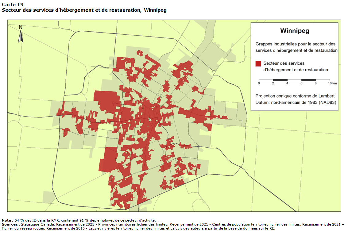
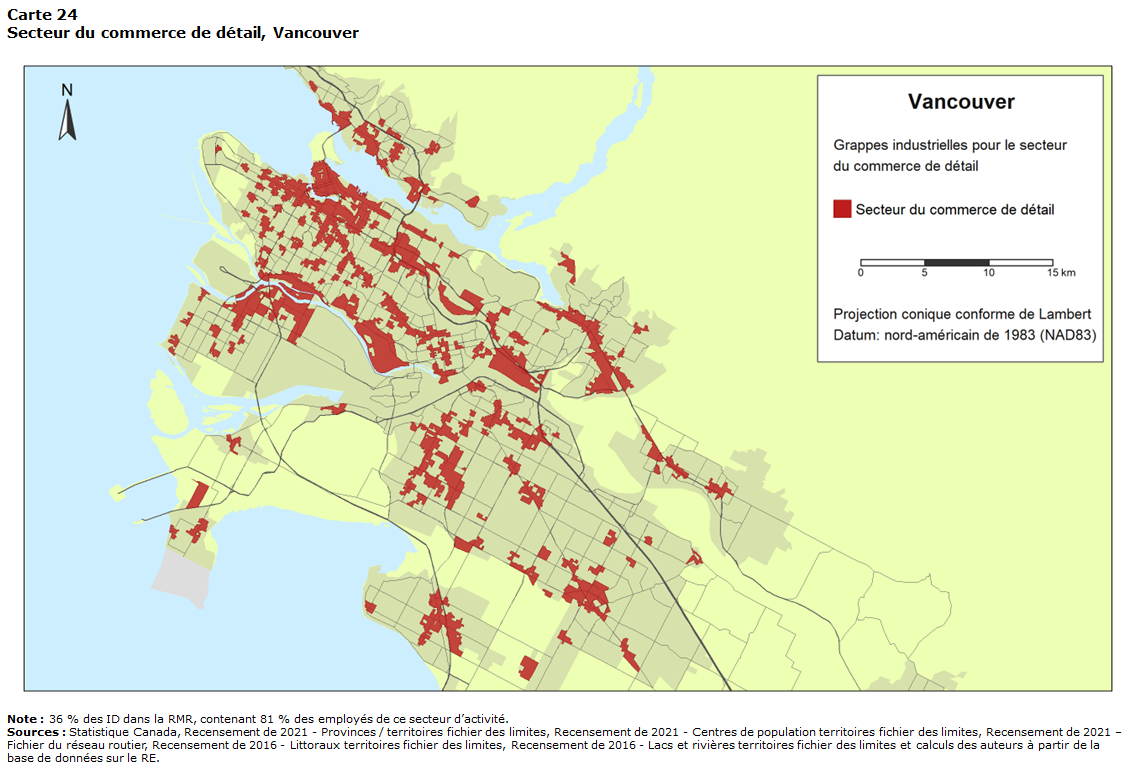
Les résultats sont cartographiés pour chaque type de grappe et de région métropolitaine montrant différentes configurations spatiales pour différents secteurs d’activité. Comme prévu, les grappes du commerce de détail et des services d’hébergement et de restauration sont relativement plus dispersées dans les régions métropolitaines que dans la grappe du secteur de la fabrication. Cependant, des statistiques simples sur les établissements et les emplois montrent que les limites géographiques des grappes à l’échelle des quartiers générées par cette analyse capturent la plupart des établissements et emplois situés dans la RMR de référence et associés à la grappe industrielle. Par exemple, la grappe du secteur de la fabrication regroupe 89,7 % (Montréal), 94,4 % (Toronto), 91,9 % (Winnipeg) et 90,8 % (Vancouver) de l’ensemble des emplois dans le secteur de la fabrication dans les RMR correspondantes. Les résultats indiquent également une colocalisation accrue de certains types d’entreprises, tels que le commerce de détail et les services d’hébergement et de restauration. Cette analyse préliminaire semble prometteuse pour révéler les schémas de colocalisation des entreprises dans les zones de quartier définies.

Les méthodes utilisées pour définir ces grappes à l’échelle des quartiers ouvrent de nouvelles possibilités d’analyse en temps opportun des conditions économiques locales ainsi que des analyses plus larges à l’échelle des quartiers (par exemple, les disparités sociales et la qualité de vie) en tenant compte de la composition des entreprises de la région. L’utilisation de fichiers de limites géographiques de grappes d’entreprises précises, comme outil de géorepérage, peut servir à surveiller la performance et les tendances des entreprises locales, en les combinant à d’autres fonds de données de Statistique Canada ou à d’autres sources de données, telles que les flux de mobilité. 

Ce projet propose une méthodologie expérimentale et un ensemble de grappes industrielles expérimentales. Vos commentaires sont appréciés. Vous pouvez communiquer vos commentaires et suggestions à l’auteur principale Jérôme Blanchet (819-576-5502), chef d'unité au Laboratoire d'exploration et d'intégration des données (LEID), et Laboratoire de données urbaines (LDU), du Centre des projets spéciaux sur les entreprise (CPSE), Statistique Canada.

Introduction

Le débat universitaire et politique sur les grappes d’entreprises s’étend sur plus de trois décennies. Dans la plupart de la littérature et des documents de politique qui en découlent, les grappes d’entreprises sont définies comme une concentration géographique d’entreprises, d’organisations et d’institutions interconnectées au sein d’une industrie ou d’un secteur particulier (Wolfe et Gertler, 2004). La théorie et les preuves suggèrent que la proximité spatiale et l’agglomération facilitent les liens de collaboration, l’échange de ressources et d’autres synergies. Ainsi, les politiques de soutien aux grappes reposent sur l’idée que le regroupement d’entreprises et d’organisations de soutien dans une zone géographique précise stimule les synergies, l’innovation et les avantages concurrentiels (Bekar et Lipsey, 2001).

La littérature concernant les grappes au Canada a étudié l’effet des grappes sur la performance des entreprises, les emplois et les salaires (Lucas et coll., 2009; Niosi et Bas, 2001; Steiner et Ali, 2011; Spencer et coll., 2010). Elle a également analysé les politiques de soutien aux grappes ainsi que leur impact et leur efficacité (Niosi et Bas, 2001) et exploré des méthodologies pour identifier et cartographier les grappes dans l’espace (Spencer, 2014). Dans l’ensemble, des documents mettent en évidence que le regroupement spatial des entreprises crée un environnement propice à l’innovation, à l’efficacité des ressources, à la collaboration et au développement économique global. Ces grappes contribuent à la croissance et au succès de chaque entreprise tout en améliorant la compétitivité et la résilience d’une région ou d’une région métropolitaine.

La plupart des documents canadiens se sont concentrés à l’échelle régionale ou sur des régions métropolitaines particulières. Pour de nombreuses applications et à des fins politiques, une analyse à l’échelle régionale (ville, région métropolitaine ou marché du travail) restera adéquate. Néanmoins, un nombre croissant d’applications nécessitent une analyse à l’échelle des quartiers et offrent des perspectives uniques tant pour les acteurs locaux (municipalités et autres organisations économiques locales) que pour les acteurs provinciaux ou fédéraux. La demande de données sur la situation et les tendances des entreprises, à des niveaux géographiques détaillés, ne cesse d’augmenter, tant de la part des organismes fédéraux que des parties prenantes locales, dont des municipalités, des associations économiques et le milieu des affaires.

La présente analyse amène l’analyse des grappes d’entreprises à un niveau géographique plus détaillé, grâce à une méthodologie mise au point pour identifier les grappes d’entreprises à l’échelle des quartiers. La méthode proposée identifie les grappes d’entreprises à l’échelle des ID, qui est l’une des unités spatiales d’analyse les plus détaillées définies par Statistique Canada^Note . Cette méthode est appliquée à quatre régions métropolitaines de recensement (RMR) de tailles différentes et pour diverses spécifications de grappes industrielles, y compris des regroupements simples de codes à deux chiffres du Système de classification des industries de l’Amérique du Nord (SCIAN), ainsi que des grappes industrielles résultant de regroupements de codes du SCIAN, tels qu’ils ont été définis par Delgado et coll. (2014).

La précision croissante de la géolocalisation pour les établissements d’entreprises dans le RE de Statistique Canada rend cette analyse possible, tandis que les possibilités offertes par le couplage de microdonnées d’entreprises ouvrent la voie à l’exploration de multiples dimensions de la performance des entreprises^Note . Dans ce contexte, l’un des principaux défis de ce type d’analyse consiste à préserver la confidentialité des renseignements confidentiels des entreprises tout en fournissant des renseignements utiles au milieu des affaires et aux décideurs. Par conséquent, cet article se veut une première exploration à l’intersection du niveau de détail le plus précis et de la protection de la confidentialité des renseignements des entreprises.

Cet article est organisé en cinq grandes sections. La section qui suit donne un aperçu des travaux existants d’analyse des grappes au Canada, mettant en lumière le manque d’information à l’échelle des quartiers ainsi que les principaux aspects motivant cette recherche, tout en proposant des exemples d’analyses à l’échelle des quartiers dans d’autres pays. Elle est suivie d’une présentation détaillée des données et de la méthodologie appliquées dans cette analyse, y compris une nouvelle approche pour le calcul de la bande passante du noyau. La section suivante présente certains résultats et valide les conclusions, avant de discuter des développements futurs et des applications possibles des délimitations de grappes. Enfin, l’annexe contient un grand ensemble complémentaire de 23 cartes de grappes à haute résolution.

Pourquoi intégrer la dimension de quartier dans l’analyse des grappes?

La plupart des études sur les grappes d’entreprises au Canada utilisent des régions ou des villes comme unités géographiques d’analyse. Pour de nombreuses applications et analyses de politiques, cette échelle géographique offre un niveau de détail adéquat. Les indicateurs de performance des entreprises sont relativement abondants à l’échelle municipale ou régionale. Au sein des villes ou des régions, on suppose que la proximité des entreprises est suffisante pour permettre les interactions qui sous-tendent le concept même de grappes et les avantages qui en découlent. Certaines des grappes bien connues, comme la Silicon Valley et le Research Triangle Park en Caroline du Nord, s’étendent sur plusieurs municipalités, et une échelle régionale semble appropriée pour étudier leur dynamique et leur développement. 

Néanmoins, des preuves montrent que certaines grappes, telles que les grappes des secteurs financiers, culturels, du commerce de détail ou de la fabrication, se concentrent dans des quartiers précis au sein d’une région métropolitaine. De même, il est établi que les disparités spatiales et les variations de performance des entreprises peuvent être aussi marquées à l’échelle des quartiers qu’à celle des régions (Wheeler, 2006; OCDE, 2018). Un grand nombre de parties prenantes et de décideurs, y compris des organisations économiques locales et des municipalités, adoptent une perspective axée sur les quartiers et élaborent ou mettent en œuvre des politiques ayant une incidence sur les entreprises dans des zones précises au sein d’une municipalité. Par conséquent, ces intervenants ont besoin d’analyses des grappes et de leur performance à des niveaux géographiques plus détaillés.

Pour répondre à ces besoins d’information, différents courants de recherche ont analysé des grappes d’entreprises à l’échelle des quartiers en examinant les choix d’emplacement dans les zones métropolitaines, l’impact des réglementations et des politiques municipales sur la formation et la croissance des grappes, le rôle des associations locales et l’impact ainsi que les retombées économiques et les effets de diffusion des grappes sur les quartiers environnants. Ces recherches s’inscrivent dans diverses perspectives disciplinaires, allant des analyses plus traditionnelles des grappes d’entreprises à des études sur l’aménagement urbain, en passant par la recherche appliquée et à l’analyse menée par des associations locales, des chambres de commerce et des services de planification municipale. Le reste de cette section fournit un aperçu de ces documents, en mettant en évidence les principaux enseignements et en soulignant les lacunes actuelles en matière d’information dans le contexte canadien.

Les disparités spatiales au sein des villes, à l’échelle des quartiers, constituent un enjeu bien connu et étudié (OCDE, 2018). Les choix des entreprises relativement à leur emplacement et leur regroupement dans certains quartiers sont influencés par ces disparités, et ils contribuent à les renforcer. Par exemple, Wheeler (2006) montre que la croissance positive des entreprises dans la région métropolitaine de St. Louis aux États-Unis, découle en réalité d’une croissance substantielle dans un quartier, combinée à un déclin dans un autre. Ces dynamiques sont motivées à la fois par les caractéristiques des quartiers et des entreprises. Ces observations sont pertinentes tant du point de vue des entreprises (pour leurs choix d’emplacement) que du point de vue de la municipalité (pour l’élaboration de politiques visant à soutenir le regroupement d’entreprises et à réduire les disparités socioéconomiques entre quartiers). L’importance d’une approche axée sur les quartiers dans l’analyse des grappes spatiales est également soulignée par Gabaix (2011), qui utilise des données d’imagerie satellitaire pour définir des grappes de densité de population. Ces résultats suggèrent que les données issues de méthodes basées sur la densité des grappes, pour délimiter les frontières urbaines, s’intègrent plus facilement dans un modèle spatial que les régions définies directement par des limites administratives. 

Les analyses des grappes d’entreprises à l’échelle des quartiers apportent des éclairages sur les choix d’emplacement des entreprises. Wheeler (2006) souligne que les investisseurs potentiels ne choisissent pas seulement une région ou une ville, mais aussi un quartier, ce qui peut, dans certains cas, correspondre à un parc industriel^Note  ou un quartier d’affaires précis. Par conséquent, la compréhension de la dynamique des parcs industriels au sein d’une région métropolitaine et de leurs environs revêt une importance particulière. Des conclusions similaires ressortent des travaux d’Arauzo-Carod (2021), qui examine les choix d’emplacement des entreprises de haute technologie à l’échelle des quartiers à Barcelone. Cette analyse montre que les caractéristiques et les installations des quartiers influencent les décisions d’emplacement des entreprises et que les retombées spatiales jouent un rôle essentiel pour certaines industries de haute technologie,

Les grappes d’entreprises ne servent pas uniquement à établir la composition économique et la disponibilité des emplois dans un quartier. Plusieurs études soulignent qu’elles peuvent également avoir une incidence sur la qualité de vie dans les quartiers et leur potentiel d’attraction à des fins résidentielles (Shybalkina, 2022; Stern et Seifert, 2010). Des travaux de recherche ont porté sur l’incidence de la présence de certaines grappes sur les quartiers, en particulier les grappes artistiques et culturelles dans les zones métropolitaines. Grodach et coll. (2014) ont identifié des grappes artistiques à l’échelle des régions et des quartiers en utilisant des codes postaux pour des zones métropolitaines américaines de tailles variées. Leurs résultats montrent que les industries artistiques présentent des schémas d’emplacement distincts à l’échelle métropolitaine et des quartiers. Ils révèlent que, bien que de nombreuses caractéristiques des grappes artistiques soient propres à un lieu, les arts sont associés à des indicateurs généraux d’innovation et de développement local, ce qui suggère que ces grappes d’entreprises peuvent jouer un rôle plus large dans le développement économique des régions métropolitaines.

Un autre courant de littérature sur les grappes d’entreprises intra-urbaines se concentre sur la délimitation et le rôle des centres d’affaires. Cette littérature est souvent regroupée sous la rubrique de l’analyse des secteurs du centre des affaires (SCDA) (Meltzer 2012; Yu et coll., 2015). Elle présente à la fois une pertinence méthodologique et politique, avec une partie axée sur les aspects de modélisation et une autre explorant le rôle et la dynamique des organisations impliquées dans la gestion, le développement et la promotion de ces centres d’affaires. Les méthodes utilisées pour délimiter les SCDA vont de l’utilisation des données de télédétection (Taubenböck et coll., 2013) aux données de recensement sur la densité des emplois (Yu et coll., 2015).

L’approche adoptée dans la présente analyse s’inspire de cette littérature et, en particulier, de l’analyse de Sergerie et coll. (2021) qui visait à élaborer une méthode pour identifier les limites géographiques des quartiers centraux de villes canadiennes. Sergerie et coll. (2021) utilisent une KDE spatiale pour calculer une surface de densité des données sur l’emplacement des emplois à l’échelle des ID, rendant possible la comparaison de ces zones partout au Canada.

La formation de grappes d’entreprises à l’échelle des quartiers, tout comme à l’échelle des régions, n’est pas simplement un processus spontané ou le résultat cumulatif d’accidents historiques. Autrement dit, ce n’est pas un phénomène aléatoire et il peut être expliqué. Les municipalités jouent un rôle clé dans le façonnement, le développement et le soutien du regroupement des entreprises dans des domaines précis (Zhang, 2019). Cela se fait généralement par l’intermédiaire du zonage, une méthode réglementaire utilisée par les municipalités ou les gouvernements locaux pour établir des règles définissant les activités et les constructions autorisées à un emplacement donné. Ainsi, les municipalités fournissent l’espace, les infrastructures et les services nécessaires au développement de parcs industriels en tant que zones dédiées à des usages industriels.

Comme les municipalités, les associations professionnelles locales sont des acteurs clés dans le soutien du développement de grappes d’entreprises locales (Dhamo et coll., 2023). À Toronto, par exemple, la Toronto Board of Trade (2021) a publié une étude cartographiant cinq types de secteurs dans la région métropolitaine élargie qui comprennent un centre métropolitain, des zones de production et de distribution de biens, des zones de services et à usage mixte, des centres régionaux et des centres de création de connaissances. Parallèlement, cette municipalité compte 84 zones d’amélioration des affaires (ZAA). Ces associations professionnelles locales visent à soutenir des zones commerciales compétitives et attrayantes pour les consommateurs et les nouvelles entreprises.

Le rôle proactif que peuvent jouer les acteurs locaux dans le développement économique et la prospérité de leur région explique pourquoi l’analyse à l’échelle des quartiers devient de plus en plus pertinente. L’analyse des grappes locales ou des concentrations d’entreprises au sein d’un quartier peut renseigner sur le comportement des consommateurs, l’emploi local et la santé économique globale du quartier. Ces acteurs locaux opèrent dans des écosystèmes géographiquement définis pour lesquels des données peuvent être générées à partir de sources locales ou analysées à l’échelle locale. Ce qui manque, particulièrement dans le contexte canadien, c’est un cadre élargi et comparatif qui permettrait l’analyse des grappes à l’échelle des quartiers à l’échelle nationale, avec des définitions normalisées dans l’ensemble des administrations. C’est ce déficit d’information que cette analyse vise à combler. Les progrès dans le géoréférencement des micro données d’entreprises et dans l’analyse spatiale de grandes bases de données facilitent de plus en plus la réalisation d’analyses détaillées à l’échelle des quartiers.

Méthodologie proposée

L’approche générale adoptée aux fins de la présente analyse s’appuie sur les travaux de Sergerie et coll. (2021) portant sur la définition des centres-villes des régions métropolitaines du Canada. Dans le cadre de ces travaux, les KDE spatiales sont appliquées à la géolocalisation du total des emplois, obtenue de la variable du lieu de travail du Recensement de la population, et l’unité géographique d’analyse utilisée est l’aire de diffusion (AD).

Dans la présente, les grappes d’entreprises sont définies à l’aide d’une méthode analogue, utilisant des KDE spatiales appliquées à la géolocalisation des emplois enregistrés à l’échelle des établissements. Les données sur les établissements sont extraites du RE pour certains secteurs et l’unité d’analyse est l’ID, une unité plus précise que l’AD. Compte tenu du niveau de détail nettement plus précis (tant pour les industries sélectionnées que pour la géographie), la méthodologie utilisée afin de définir les grappes d’entreprises comporte plusieurs étapes supplémentaires par rapport au flux de travail décrit par Sergerie et coll. (2021). Les sections suivantes décrivent en détail la méthodologie proposée. 

Zones d’étude

Quatre zones d’étude, représentant différents degrés de densité urbaine au Canada, ont été sélectionnées pour mettre au point la méthodologie. Il s’agit des RMR de Montréal, de Toronto, de Winnipeg et de Vancouver. Chaque RMR comprend un nombre différent de municipalités (subdivisions de recensement), avec des quartiers présentant des densités de population et d’emploi, ainsi que des degrés d’urbanisation, sensiblement différents. 

L’unité géographique d’analyse utilisée pour la géolocalisation des entreprises est l’ID. Un ID est un territoire dont tous les côtés sont délimités par des routes et/ou par des limites; dans les zones urbaines, c’est ce que l’on appelle communément un « îlot ». Les ID font partie des régions géographiques normalisées de Statistique Canada aux fins de diffusion et ils sont la plus petite région géographique pour laquelle les chiffres de population et des logements sont diffusés. Les îlots de diffusion couvrent tout le territoire du Canada^Note .

Registre des entreprises

Les données utilisées dans l’analyse proviennent du RE de Statistique Canada, qui est le répertoire central de données de base sur les entreprises et les établissements ayant des activités au Canada. Il est continuellement mis à jour. Pour cette analyse, les données se rapportent à la période de référence de décembre 2023.

Dans le RE, les secteurs d’activité sont définis selon les codes du SCIAN. L’utilisation des données du RE présente des avantages par rapport à d’autres sources de données possibles, comme les données sur le lieu de travail du Recensement de la population. Les données à l’échelle des établissements du RE sont classées selon des codes du SCIAN plus détaillés (à six chiffres), ce qui permet la création de grappes personnalisées. Les données sur l’emploi dans le RE sont également mises à jour plus fréquemment. Bien qu’elles soient moins précises que les statistiques sur l’emploi spécialisées, elles constituent une solution de rechange plus opportune aux données du recensement. 

Les codes du SCIAN inclus dans cette analyse représentent six grappes industrielles différentes. Trois d’entre elles sont composées de codes du SCIAN à deux chiffres et les autres sont définies selon les travaux de Delgado et coll. (2014). Ces grappes industrielles et leurs codes du SCIAN correspondants sont résumés dans le tableau 1.

Les grappes industrielles générées à l’échelle des codes du SCIAN à deux chiffres comprennent le secteur de la fabrication (SCIAN 31, 32 et 33), le secteur du commerce de détail (SCIAN 44 et 45) et le secteur des services d’hébergement et de restauration (SCIAN 72).

Les trois grappes industrielles définies selon Delgado et coll. (2014) sont les suivantes : premièrement, la distribution et le commerce électronique (grappe 10). Cette grappe comprend principalement les grossistes traditionnels, les maisons de vente^Note  par correspondance et les marchands électroniques. Les entreprises de cette grappe achètent, stockent et distribuent principalement une large gamme de produits, tels que des vêtements, des aliments, des produits chimiques, du gaz, des minéraux, des matériaux agricoles, des machines et d’autres marchandises. La grappe comprend également des entreprises qui soutiennent les opérations de distribution et de commerce électronique, y compris l’emballage, l’étiquetage et la location de matériel. La deuxième grappe est celle des services financiers (grappe 16). Elle comprend des établissements qui aident à la transaction et à la croissance d’actifs financiers pour les entreprises et les particuliers. Ces sociétés comprennent des courtiers en valeurs mobilières, des négociants et des bourses, des institutions de crédit et des services de soutien à l’investissement financier. Les sociétés d’assurance sont regroupées dans une autre grappe, celle des services d’assurance. Enfin, le secteur de l’hôtellerie et du tourisme (grappe 22) comprend des établissements liés aux services et aux lieux de l’hôtellerie et du tourisme. Cela inclut des sites sportifs, des casinos, des musées et d’autres attractions, ainsi que des hôtels et autres types d’hébergement, des transports, et des services liés aux voyages récréatifs, tels que les services de réservation et les voyagistes.

La structure hiérarchique entre les 3 grappes d’industries générées au niveau du SCIAN à 2 chiffres et la grappe à 3 industries définie selon Delgado et coll. (2014) n’est pas simple. C’est-à-dire que les différents niveaux à 4 chiffres du SCIAN utilisés selon Delgado et coll. (2014) ne sont pas nécessairement composés des premiers niveaux à 2 chiffres 31, 32, 33, 44, 45 et 72. De plus, pour des raisons de commodité et de simplicité, la récurrence des 6 grappes industrielles n’est pas nécessairement la même dans le présent document. C’est-à-dire que certaines étapes de l’analyse des résultats et de la méthodologie se concentrent sur les 3 grappes industrielles générées au niveau à 2 chiffres du SCIAN seulement, tandis que d’autres se concentrent sur les 6 grappes industrielles.

Estimation de la densité

La concentration spatiale des industries a été déterminée à l’aide d’une méthode de KDE spatiale. Il s’agit d’une technique non paramétrique qui estime la fonction de densité de probabilité d’une variable aléatoire sur un domaine spatial. Pour chaque région métropolitaine, des grappes ont été identifiées à l’aide des résultats de la méthode de KDE en agrégeant les ID adjacents ayant une densité minimale d’emploi dans chaque secteur ou combinaison de secteurs.   

Les données sur l’emploi provenant des données des établissements du RE ont été géocodées en fichiers de limites spatiales des ID. Le nombre total d’employés par ID a ensuite été calculé. Les lieux des emplois représentant chaque employé ont été distribués de façon aléatoire et uniforme dans la limite de l’ID^Note . Cette étape de traitement doit être reconnue, non pas comme un manque de précision et une faiblesse des données, mais comme un moyen de faire progresser la méthodologie. En d’autres mots, cette méthode permet de rendre plus homogène la distribution spatiale relativement clairsemée des emplois dans l’ID et facilite le processus de KDE en générant une distribution relativement plus continue ^Note . L’argument de l’uniformité a été avancé pour ne privilégier aucune sous-région de l’ID pendant le processus de randomisation. Cela signifie que la concentration de la densité des établissements dans certains points précis de l’ID n’influence pas le processus de randomisation des emplois. Certaine section ci-bas de ce rapport décrive en plus grand détails les processus de distribution de données aléatoires.

La section d’estimation de la densité de cet article est composée de 2 sous-sections. Tout d’abord, nous documentons des informations partielles sur la fonction de densité du noyau polynomiale. Juste assez d’arguments de fonction pour comprendre l’utilité de la taille de la bande passante du noyau. Nous expliquons également pourquoi l’approche de la bande passante du noyau Silverman n’est pas adaptée à notre application, puis nous décrivons une nouvelle méthode pour le calcul de la bande passante. Deuxièmement, nous décrivons toutes les informations sur la fonction de densité du noyau polynomiale. C’est-à-dire tous les arguments restants de la fonction non décrits jusqu’à présent. Nous documentons également les processus aléatoires utilisés.

Méthodologie de bande passante de densité du noyau et autres paramètres

Avant de décrire la version entière de la méthode KDE, nous détaillons partiellement la fonction de densité de noyau polynomiale $\text{PKDF}(\text{Φ},\text{Φc},\text{ψ)}$ qui constitue l’instrument principal de la méthode KDE. La fonction nécessite un minimum de trois arguments : l’identifiant de la cellule de sortie de la grille $\text{Φ}$, le centroïde de la cellule de sortie de la grille $\text{Φ}\text{c}$, et enfin la bande passante ou le rayon $\text{ψ}$. La forme fonctionnelle polynomiale a été retenue selon Sergerie et coll. (2021), bien que des formes normale et uniforme aient été disponibles. $\text{Φ}\text{c}$ a été définie comme géométrique, sans pondération selon la concentration de la densité spatiale des établissements dans l’ID et non pondérée en fonction de la concentration de densité spatiale de l’établissement de l’ID. Plusieurs spécifications et essais pour $\text{Φ}$ et $\text{ψ}$ ont été envisagés afin de garantir l’interprétabilité économique des résultats et l’efficacité de calcul. Ceux-ci sont brièvement documentés ci-dessous.

La dimension d’une cellule (ou tuile) pour une grille $\text{G}$ est un paramètre de choix. Aux fins de cette analyse, une grille carrée dont la dimension des cellules est de 50 x 50 mètres a été adoptée. Après l’essai de différentes spécifications (p. ex. une plage de 10 x 10 à 100 x 100 mètres), la grille de 50 x 50 mètres a été adoptée pour trouver un équilibre entre le détail spatial et l’efficacité de calcul. La Figure 1 ci-dessous illustre la distribution du nombre de cellules de 50 x 50 mètres par l’ID dans les quatre régions métropolitaines. La Figure confirme qu’un nombre minimal et raisonnable de cellules sont disponibles dans la majeure partie de l’ID de chaque RMR. En outre, le nombre médian de cellules par ID varie de 7,5 à 12,5. Enfin, la Figure montre également les variations entre les RMR quant au nombre total de cellules pouvant s’intégrer dans un seul ID. Cette variation est particulièrement importante, car elle représente les caractéristiques des grandes et des petites RMR au Canada. Les petites RMR présentent généralement une gamme plus étendue de dimensions d’ID, tandis que les grandes RMR de l’étude ont une gamme plus restreinte et plus petite de dimensions d’ID. Il est intéressant de noter que Montréal est la seule RMR à afficher une distribution symétrique des ID, contrairement aux trois autres RMR où la distribution est plus asymétrique.

Description de la figure 1

Table 01
Sommaire du tableau
Le tableau montre les résultats de Table 01 , calculées selon (figurant comme en-tête de colonne).

	"RMR de Montréal CMA"	"RMR de Toronto"	"RMR de Winnipeg"	"RMR de Vancouver"
Source : calculs des auteurs à partir de la base de données sur le RE.
Minimum	0	0	0	0
Premier trimestre	4	5	6	6
Median	8	9	12	9
Moyenne	53,12	76,26	249,4	77,41
Troisième trimestre	14	22	48	21
Maximum	11 357	38 258	37 816	162 076

De même que le choix de la dimension des cellules de la grille, le choix de la bande passante du noyau, $\text{ψ}$ , a des implications sur les résultats. On peut comparer cela à un histogramme simple : une bande passante trop grande (équivalente à un histogramme avec très peu de barres) masque la distribution sous-jacente. À l’inverse, une bande passante trop petite peut entraîner une fréquence de 1 unité pour chaque résultat, rendant difficile la compréhension de la distribution des données avec un histogramme trop aplati.    

Pour définir $\text{ψ}$, diverses spécifications ont été mises à l’essai, notamment la célèbre règle empirique de Silverman (1986), appliquée dans l’étude de Sergerie et coll. (2021). Compte tenu de la taille des cellules de la grille et de la configuration des ID utilisées dans notre analyse, la bande passante calculée par Silverman n’a pas permis d’inclure suffisamment de données dans son environnement local. Cela a entraîné une distribution spatiale insuffisamment lissée des lieux des emplois, rendant la méthode KDE inefficace et générant des grappes fragmentées. Le paragraphe suivant propose une interprétation des raisons pour lesquelles le processus de Silverman n’a pas fourni une taille de bande passante satisfaisante pour nos applications dans cette recherche.

L’équation de Silverman saisit la dispersion des lieux des emplois autour d’un point de référence dans la RMR. De la section précédente, nous savons que les lieux des emplois sont initialement géocodés à la localisation spatiale fixe de leurs établissements respectifs, puis distribués de manière aléatoire et uniforme dans les limites de leurs ID respectifs, sans donner la priorité au lieu de l’établissement ou à une sous-région précise de l’ID. Par conséquent, nous pouvons affirmer que l’équation de Silverman encapsule des renseignements partiels sur la distribution de la dimension des ID dans la RMR. Cependant, l’équation ne prend pas nécessairement en compte la dimension d’un ID type, qu’il s’agisse d’un ID moyen ou médian. Par conséquent, dans les exemples précis de nos applications, la bande passante de Silverman ne parvient pas à agréger les données entre les ID et propose uniquement une transformation des données du noyau dans les limites de l’ID de référence, laissant les résultats finaux à l’échelle des ID inchangés par rapport aux données d’origine du RE.  

Nous proposons rapidement une interprétation de ce problème expliquant pourquoi la bande passante est trop petite. La bande passante de Silverman est définie par ${\text{0,9m/s}}^{\text{1/5}}$, où $\text{s}$ est la taille de l’échantillon et $\text{m }=\text{min}{\left(\text{σ}, {\left(1/\text{ln}\left(2\right)\right)}^{1/2}*\text{ μ}\right)}^{1/2}$. Ici, $\text{σ}$ est la dispersion standard de la distribution des points de données spatiales d’emploi $\text{X}$ par rapport au point central moyen unique de la RMR et $\text{μ}$ est le moment statistique de dispersion médiane (50e centile) dans la distribution de la dispersion de $\text{X}$ au centre moyen. Il convient de noter qu’une autre version de l’équation de Silverman remplace la médiane $\text{μ}$ par l’intervalle interquartile $\text{IQR()}$, où $\text{IQR() = 75\%}$ centile moins 25 % centile.

Autrefois, l’équation non pondérée pour la distance standard était,

$$\text{σ }=\sqrt{({\displaystyle \sum }_{\text{j}=1}^{\text{s}}\frac{{\left(\text{L}1\left(\text{j}\right)-\text{L}1\text{C}\right)}^2}{\text{s}}+{\displaystyle \sum }_{\text{j}=1}^{\text{s}}\frac{{\left(\text{L}2\left(\text{j}\right)-\text{L}2\text{C}\right)}^2}{\text{s}})}$$

où $\text{L}1$ et $\text{L}2$ sont les coordonnées numériques de longitude et de latitude des éléments de $\text{X}$, respectivement, et $\text{L}1\text{C}$ et $\text{L2C}$ sont les coordonnées numériques de longitude et de latitude du centre moyen de la RMR respectivement. Intuitivement, $\text{σ}$ et $\text{μ}$ ne peuvent pas être contenus dans un ID type ou médian de la RMR parce que les lieux des emplois sont largement disponibles spatialement sur l’ensemble des superficies de la RMR. Par conséquent, nous supposons que le minimum (min) des deux quantités est raisonnablement assez grand et ne peut pas expliquer une taille de bande passante Silverman trop petite. D’autre part, la taille de l’échantillon $\text{s}$ Figure au dénominateur de la formule de Silverman et $\text{s}$ peut fournir une très petite bande passante si $\text{s}$ est trop grand. La distribution du nombre d’employés par établissement dans le RE peut être fortement asymétrique à droite, comprenant des valeurs aberrantes positives atteignant des valeurs très élevées, ce qui contribue à une valeur $\text{s}$ très grande en raison de l’épaisseur de l’extrémité droite de la distribution. Par conséquent, si $\text{s}$ est assez grand pour maintenir ${\text{s}}^{1/5}$ assez élevé, alors la bande passante sera petite, et irréaliste. Cette étude ne s’attarde pas sur le processus d’élimination des valeurs aberrantes des données du RE, mais cela pourrait faire l’objet d’une étude future. Plus précisément, l’application des travaux publiés par Statistique Canada, tels que Outliers in Sample Surveys de Lee et coll. (1992), A Cautionary Note on Clark Winsorization de Mulry et coll. (2016), A Method of Determining the Winsorization Threshold with an Application to Domain Estimation de Martinoz et coll. (2015), et On Searls’ Winsorized Mean for Skewed Populations de Rivest et coll. (1995), est pertinente. Il convient également de noter que l’équation de Silverman est adaptée aux valeurs de densité du noyau normalement distribuées, ce qui n’est pas le cas pour notre distribution de densité asymétrique extrêmement droite présentée ci-dessus. Enfin, il faut souligner que Mathematica utilise une modification de l’équation de Silverman, $\text{0,09}*\text{σ}$, pour de grands échantillons $\text{s}$ dépassant 100 000 observations. Cependant, nous n’avons pas utilisé le logiciel analytique Mathematica pour cette recherche et avons décidé de ne pas tirer parti de cette version de l’équation de Silverman. Intuitivement, la suppression du grand échantillon $\text{s}$ du RE au dénominateur du rapport de Silverman contribuerait à résoudre le problème d’un dénominateur trop grand et d’une bande passante trop petite, si le remplacement d’un coefficient de 0,9 par 0,09 (réduction d’environ 90 %) ne réduit pas trop la bande passante.  

Pour résoudre le problème lié à la règle empirique de Silverman dans nos applications, cette recherche développe sa propre méthodologie de bande passante qui se concentre sur la distribution des superficies d’ID fournies par les données. En d’autres termes, notre bande passante personnalisée tient compte de la dimension de l’ID médian dans la RMR de référence^Note . Cette nouvelle approche garantit que la bande passante est suffisante pour couvrir à la fois un ID type et les ID des quartiers. Cette condition est fondamentale, car le produit final de ce projet se situe à l’échelle de l’ID. Par conséquent, si la densité de chaque cellule de la grille représente uniquement l’agrégation des renseignements situés dans les limites de leur ID respectif, aucune information spatiale exclusive ne serait générée par cette recherche. 

La Figure 2 illustre la méthode de la bande passante élaborée pour la présente analyse. La grille $\text{G}(\text{m}\text{D}\text{B})$ remplie d’ID, à ne pas confondre avec la grille des cellules de sortie $\text{G}$ susmentionnée, suppose un environnement local avec des ID au carré égaux dont les dimensions sont celles de l’ID médian empirique de la RMR de référence. L'ID médian est dérivée d'une zone projetée dans le système de référence de coordonnées (CRS) EPSG:3347. $\sqrt{\text{A}}$ est la longueur latérale d’un ID médian. Par conséquent, $\sqrt{\text{A}}*\sqrt{\text{A}}$ est le volume ou les superficies d’un ID médian. Les points rouges sont les centroïdes géométriques des cellules de la grille dans un ID médian de la grille $\text{G}(\text{m}\text{D}\text{B})$ et ne doivent pas être confondue avec le centroïde géométrique d’un ID.  

En se basant sur l’exemple à gauche, la bande passante n^o 2, représentée par un cercle, parvient à couvrir l’intégralité des renseignements demandés, mis en évidence en gris et en jaune. C’est-à-dire que la bande passante couvre l’intégralité de l’ID de référence de la cellule et de ses huit ID voisins directs, respectivement. Il convient de noter qu’il s’agit de la bande passante la plus petite possible pour satisfaire à ces conditions. Plus précisément, cela couvre $\left(14,137\text{*A}\right)/\left(9\text{*A}\right)=1,57$ fois la superficie demandée. Le calcul de la longueur de la bande passante repose sur une logique de distance euclidienne simple; $\text{B }=\sqrt{\text{A}}\text{ * }1,5$ par conséquent $\text{C}=\text{ψ} =\sqrt{\left({\text{B}}^2+{\text{B}}^2\right)}$. Cette logique garantit qu’un centroïde d’une cellule de sortie de la grille qui se superpose au centroïde géométrique de l’ID pourra capter toutes les données nécessaires. En outre, en se basant sur l’exemple de droite de la Figure 2, la cellule de sortie de la grille se situe maintenant dans le coin supérieur droit du même ID de référence. La bande passante n^o 2 parvient à couvrir tous les ID demandés, à l’exception d’un ID situé en bas à gauche, dont la superficie est accessible à 50 %. Cette zone inaccessible est considérée comme acceptable dans notre méthodologie, car les nouveaux ID deviennent maintenant accessibles en haut à droite, même s’ils ne sont pas un voisin direct de l’ID de référence. 

Les cartes thermiques des grappes produites à l’aide de cette nouvelle méthode de bande passante ont donné une surface lisse tout en préservant les détails des quartiers (voir les détails en annexe). Pour plus de clarté, la présente analyse reconnaît la notation de la bande passante sous la forme $\text{ψ}\left(\text{mDB}\left(\text{RMR}\right)\right)$, puisque le rayon personnalisé dépend maintenant d’un seul argument : la configuration de l’ID médian (IDM), et l’IDM est lui-même adapté à chaque RMR. C’est-à-dire que la bande passante varie d’une RMR à l’autre, mais reste fixe au sein de chaque RMR, quelle que soit la variance de la concentration des lieux des emplois dans les quartiers de la RMR. Cependant, la notation $\text{ψ}$ restera en usage pour des raisons d’efficacité spatiale. Enfin, il convient de noter que notre bande passante personnalisée $\text{ψ}$ ne dépend pas de la dispersion des lieux des emplois. Par conséquent, si les RMR A et B ont le même IDM et que la RMR B a deux fois plus de dispersion des lieux des emplois que la RMR A, alors les deux RMR obtiendront la même $\text{ψ}$, ce qui est inapproprié parce que la dispersion des lieux des emplois a son importance. D’autre part, notre bande passante personnalisée est robuste aux grandes valeurs aberrantes dans la distribution du nombre d’employés par établissement du RE. Une amélioration de notre bande passante comprendrait à la fois une dépendance à l’IDM et la dispersion des lieux des emplois.    

Description de la figure 2

Source : calculs et méthodologie des auteurs.
Legend:
$\text{Longueur latérale d'un ID médian}=\sqrt{\text{A}}$ ,
$\text{A }=\text{ Superficie médiane de l'ID}=\sqrt{\text{A}}\text{ * }\sqrt{\text{A}}$,
$\text{B}=\sqrt{\text{A}}\text{ * }1,5$ $\text{C }=\text{ ψ}=\sqrt{\left({\text{B}}^2+{\text{B}}^2\right)}$ , et
$\text{C }=\text{ ψ}=\sqrt{\left({\text{B}}^2+{\text{B}}^2\right)}$

Processus aléatoires multinomiaux uniformes et fonction de densité de noyau polynomiale

À la suite de la spécification des arguments $\text{Φ}$, $\text{Φ}\text{c}$ , et $\text{ψ}$, cette section documente le reste des détails de la fonction de densité de noyau polynomiale spatial (PKDF) appliqué dans l’analyse^Note . Ce modèle de densité de noyaux est en partie inspiré par Sergerie et al. (2021) concernant la façon d’appliquer un modèle de densité de noyaux à une population granulaire d’entreprises au Canada, Cependant, il prend la structure fondamentale des statisticiens Emanuel Parzen (1962) et Murray Rosenblatt (1956) qui ont créé indépendamment la forme théorique de densité du noyau.  La notation utilisée est la nôtre. Cet article porte sur une contribution appliquée, avec la génération des cartes thermiques des clusters. Cet article n’a aucune contribution théorique, en dehors de la conception de la bande passante du noyau (présentée ci-dessus). Cet article utilise plusieurs résultats existants de la littérature pour l’explication des termes et concepts mathématiques théoriques de la densité du noyau, et pour l’explication des processus aléatoires appliqués avant le modèle de densité du noyau (expliqués ci-dessous), dans le cadre d’une population spatial de polygone d’ID et de localisation des emplois. Les termes restants à expliquer ci-dessous sont : $\text{i}$, $\text{n}()$, $\text{J}\text{W}()$, $\text{J}\text{L}()$, $\text{J}$, $\text{Θ}()$ et $\text{r}()$.

$\text{n}\left(\text{Φ},\text{Φc},\text{ψ}\right)$ représente le nombre fini non négatif des emplacements d’emplois disponibles dans l’environnement circulaire et symétrique ${\text{πψ}}^2$ de la cellule ciblée de sortie de la grille $\text{Φ}$ et inclus dans le calcul de la densité totale de la cellule. Par conséquent, $\text{n}()$ dépend de l’identifiant de la cellule de sortie de la grille évalué $\text{Φ}$ , de l’emplacement du centroïde géométrique de la cellule $\text{Φ}\text{c}$ et de la longueur de la bande passante du noyau $\text{ψ}$. Par conséquent, le nombre d’ID qu’il couvre variera en fonction de l’endroit où $\text{Φ}$ se situe. Il peut couvrir plusieurs ID ou moins d’un ID. i représente l’indice des emplois uniques inclus dans $\text{π}{\text{ψ}}^2$ autour de la cellule ciblée de sortie de la grille $\text{Φ}$ et ne peut aller que de 1 à $\text{n}\text{()}$.   

Les pages suivantes documentent les processus aléatoires utilisés dans notre méthodologie. Cette documentation est importante pour comprendre la structure de ces processus. $\text{JL}\left(\text{i}\right)~\text{U}\left(\text{DBP}\right)$ représente le lieu géographique de l’emploi i, qui, dans le cadre de l’estimation de la densité du noyau, est distribué de manière uniforme et aléatoire $\text{(U())}$ sur la superficie du polygone de l’ID. Il ne se trouve pas nécessairement à l’emplacement de l’établissement d’origine auquel l’emploi i appartient. De plus, le lieu de l’emploi ne peut pas être distribué de manière aléatoire en dehors des limites de son propre ID, ni même à l’intérieur des limites de sa propre AD. En outre, tous les lieux des emplois i compris entre $\text{i}=1$ et $\text{i}=\text{n}$ et appartenant au même ID sont i,i,d, c’est-à-dire indépendants et identiquement distribués à partir de la même distribution spatiale. Nous nommons ce processus aléatoire RP.

$\text{J}\text{L}()$ est i.i.d. en ce sens qu’un emplacement de travail unique peut être attribué spatialement et aléatoirement indépendamment de l’emplacement aléatoire spatial d’un autre emploi unique. Cependant, comme nous l’expliquerons plus loin dans cet article, le processus aléatoire doit également être considéré comme le nombre d’emplois uniques attribuées au hasard sur un point spatial spécifique de l’ID. Dans cette perspective, plus le nombre de d’emplois uniques attribuées au hasard sur un point spatial spécifique est important, moins il est probable qu’un autre point spatial obtienne de nombreux emplois, car le nombre d’emplois uniques d’un ID est fini et non infini. Pour cette raison, l’idée clé est de visualiser les phénomènes comme des points de données (un grand ensemble d’emplois uniques) attribués aléatoirement aux multi-catégories (plusieurs points spatiaux sur un ID) d’une variable aléatoire multinomiale (un ID).

Quelques perspectives concernant le processus aléatoire (RP) méritent d’être mentionnées. Bien qu’il soit uniforme, le RP ne génère pas toujours une couverture uniforme pour un ID, certains quartiers de l’ID pouvant être plus couverts que d’autres. Plus précisément, l’événement le plus probable de notre processus RP est une allocation spatialement uniforme de points de données au sein de l’ID, où chaque point spatial reçoit le même nombre d’emploi. C’est notre événement attendu $\text{E}\left(\text{RP}\right)$. D’autre part, l’événement le moins probable, mais toujours possible, se produit lorsque tous les points de données distincts se superposent à un endroit unique de l’ID. Il s’agit de notre événement exceptionnel $\text{T}\left(\text{RP}\right)$.  

Exemple pour ID de petite taille avec un processus aléatoire binomial uniforme

Pour mieux comprendre le processus aléatoire RP de notre méthodologie, une analogie peut être fournie avec un processus aléatoire binomial uniforme simple BRP avec $\text{b}$ unique très petit ID de 2 espace spatial et $\text{v}$ emploi unique par ID, où $\text{v}$ est un grand nombre pair et $\text{b}$ est un grand nombre. Pour construire l’intuition de manière simple, nous analysons principalement l’événement attendu et le plus rare de la distribution, et quelques autres événements entourant l’événement attendu et le plus rare, et non d’autres détails de la distribution. Analogiquement, une pièce de monnaie non biaisée propose un processus spatial uniforme composé de 2 points puisque les deux côtés de la pièce ont une probabilité égale et qu’il n’y a pas de priorité pour l’un des 2 côtés. Cependant, il n’y a aucune garantie que l’attribution pour pile et face sera uniforme, tout le temps. L’événement le plus probable est un mélange parfait de pile et de face. C’est-à-dire que l’événement attendu $\text{E}\left(\text{BRP}\right)$ est une situation où chaque côté de la pièce reçoit une allocation égale de $\text{v/2}$ emplois uniques. Cette situation arrivera à une très grande proportion des $\text{b}$ ID. D’un autre côté, l’événement le plus improbable, mais toujours possible, est d’obtenir tous les $\text{v}$ emplois d’un seul côté de la pièce (soit face, soit pile). C’est-à-dire que tous les emplois uniques sont attribués au hasard sur le même des 2 points spatiaux disponibles. Cette situation est notre événement $\text{T}\left(\text{BRP}\right)$ et cela arrivera à une très petite proportion des $\text{b}$ ID. Intuitivement, toutes les combinaisons possibles de $\text{v}$ emplois attribuées sur l’espace spatial pile et face ont la même probabilité de réalisation, mais puisque l’événement de $\text{v}$ pile ou $\text{v}$ face est de 1 combinaison possible, respectivement, et que l’événement d’un mélange parfait de pile et de face est un très grand nombre de combinaisons distinctes, L’événement mixte parfait est alors plus susceptible de devenir l’événement attendu.

Formellement, nous avons la structure de nombre de possibilités suivante,   

$${\displaystyle \sum }_{\text{j}=0}^{\text{v}}\text{C}\left(\text{v},\text{j}\right)= {\displaystyle \sum }_{\text{j}=0}^{\text{v}}\frac{\text{v}!}{\left(\text{j}\right)!\left(\text{v}-\text{j}\right)!}>\text{E}\text{c}\left(\text{B}\text{R}\text{P}\right)=\text{C}\left(\text{v},\frac{\text{v}}{2}\right)=\frac{\text{v}!}{\left(\frac{\text{v}}{2}\right)!\left(\text{v}-\frac{\text{v}}{2}\right)!}>\text{T}\text{c}\left(\text{B}\text{R}\text{P}\right)=\text{C}\left(\text{v},0\right)=\frac{\text{v}!}{\left(0\right)!\left(\text{v}-0\right)!} = \text{C}\left(\text{v},\text{v}\right)=\frac{\text{v}!}{\left(\text{v}\right)!\left(\text{v}-\text{v}\right)!}=1$$

Où $\text{C}\left(\text{v},\text{j}\right)=\left(\begin{array}{c}\text{v}\\ \text{j}\end{array}\right)$, est le nombre de façons de choisir $\text{j}$ élément parmi $\text{v}$ élément sans ordre^Note  , l’inégalité de droite ( $>$ ) est pour les événements les plus rares, l’inégalité du milieu ( $>$ ) est pour l’événement attendu, l’égalité de gauche ( $>$ ) est pour le nombre total de combinaisons possibles, et l’indice j de valeur 0 et de valeur $\text{v}$ est pour $\text{v}$ pile et $\text{v}$ face,  respectivement. À titre d’analyse supplémentaire, notons que $\text{C}\left(\text{v},\frac{\text{v}}{2}-1\right)\text{= C}\left(\text{v},\frac{\text{v}}{2}+1\right)$ représentent le nombre de combinaisons pour des événements qui sont à un pas d’une allocation spatiale parfaitement équilibrée, respectivement, et qui sont tout aussi moins susceptibles de se produire que l’événement attendu lié au nombre de combinaisons $\text{C}\left(\text{v},\frac{\text{v}}{2}\right)$ mais toujours très susceptibles de se produire en probabilité et assez proches de la probabilité d’événement attendu. De la même manière, $\text{C}\left(\text{v},0+1=1\right)=\text{C}\left(\text{v},\text{v}-1\right)$ peut être considéré comme le nombre de combinaisons pour des événements qui sont un pas en avant d’une allocation spatiale plus uniforme, respectivement, et encore très peu probables de se produire, mais beaucoup plus susceptibles de se produire que le $\text{T}\left(\text{BRP}\right)$ (Grimaldi, 2003).

Nous devons également visualiser l’analyse en termes de somme de variables aléatoires de même pondération (moyenne non pondérée). C’est-à-dire que si nous étiquetons chacun des 2 points spatiaux de l’ID avec les valeurs numériques +1 et -1, alors pour l’événement attendu E(BRP), le nombre de +1 est égal au nombre de -1 et la moyenne est,

$$\left(\left(+1\right)\text{ * }\left(\text{v}/2\right)+\left(-1\right)\text{ * }\left(\text{v}/2\right)\right)/\text{ v}=0$$

Si nous nous éloignons d’un pas d’une allocation spatiale parfaitement équilibrée, nous avons une moyenne de,

$$\left(\left(+1\right)\text{*}\left(\left(\text{v}/2\right)-1\right)+\left(-1\right)\text{*}\left(\left(\text{v}/2\right)+1\right)\right)/\text{ v }\text{et }\left(\left(+1\right)\text{*}\left(\left(\text{v}/2\right)+1\right)+\left(-1\right)\text{*}\left(\left(\text{v}/2\right)-1\right)\right)/\text{ v}$$

qui sont différentes d’une moyenne de 0, respectivement, mais toujours proches de 0, respectivement.    

Pour T(BRP), nous obtenons soit la valeur numérique -1,  fois d’affilée, soit la valeur numérique +1, v fois d’affilée, et la moyenne est respectivement,

$-1=\left(-1*\text{v}\right)/\text{ v}$ et $+1=\left(+1*\text{v}\right)/\text{v}$

Si nous avançons d’un pas vers une allocation spatiale plus uniforme, nous avons une moyenne de,

$\left(\left(-1\right)*\left(\text{v}-1\right)+\left(+1\right)*\left(1\right)\right)/\text{v}$ et $\left(\left(+1\right)*\left(\text{v}-1\right)+\left(-1\right)*\left(1\right)\right)/\text{v}$

qui sont différentes d’une moyenne de -1 et +1 respectivement, mais toujours proches de -1 et +1, respectivement.  

Nous comprenons maintenant que la distribution d’ID ne concerne pas seulement une allocation spatiale parfaitement uniforme pour chaque ID de la RMR et qu’une dégradation symétrique et lisse de l’uniformité est présente des deux côtés (gauche et droite) de l’événement moyen, si le nombre d’emplois dans chaque ID est grand et si le nombre d’ID dans la RMR est grand. En répétant l’exercice pour l’ensemble du support de la distribution (et pas seulement pour les événements moyens et les plus rares), on obtient la forme d’une distribution approximative de la courbe en cloche. Il est maintenant temps de relier le théorème central limite univarié existant pour la distribution binomiale et sa variance finie à notre explication^Note . Autrement dit, asymptotiquement, si $\text{v }\to \text{∞}$, alors BRP converge en distribution vers la distribution normale univariée ($\text{BRP}\to \text{ N}()$)^Note . Dans un contexte fini, si $\text{v}$ est suffisamment grand, nous pouvons approximer BRP^Note  de telle sorte que^Note ,  

$$\text{BRP}\approx \text{N}\left(\text{v * }0.5,\text{ v * }0.5\text{ * }0.5\right)$$

Où le terme 0.5 représente l’égalité des chances d’attribuer un emploi sur l’un des 2 points spatiaux de l’ID, le terme $\text{v}*0,5$ représente le nombre prévu d’emploi à attribuer sur l’un des 2 point spatial, ce qui représente la moitié du nombre total d’emploi uniques disponibles pour tous les établissements de l’ID, et où $\text{v}*0,5*0,5$ représente la variance du nombre d’emploi allouées sur l’un des 2 points spatial de l’ID (Severini, 2005). Enfin, dans un contexte fini, nous pouvons nous attendre à observer une distribution normale approximative réalisée à travers l'ensemble des ID d'une grande RMR si b est suffisamment grand dans la RMR et $\text{v}$ est suffisamment grand dans chaque ID de la RMR, ou, dans un contexte théorique, une distribution normale si $\text{b}\to \text{∞}$ dans la RMR et $\text{v}\to \text{∞}$ dans chaque ID de la RMR. Ce paragraphe conclut notre exemple de processus aléatoire binomial.  

Processus aléatoires multinomiaux uniformes pour un ID de grande taille

Les calculs mathématiques pour notre processus aléatoire principal RP sont une idée similaire, mais utilisent un processus multinomial uniforme (avec variance finit) au lieu d’un processus binomial uniforme (avec variance finit) car le nombre de points spatiaux par ID est fini^Note  et grand et pas seulement égal à 2. De plus, d'après le théorème central limite multivarié (TCLM) existant pour le processus multinomial, si $\text{v}\to \text{∞}$, alors la convergence en distribution du processus multinomial uniforme est une distribution normale multivariée plutôt qu'une distribution normale univariée (Severini, 2005) ($\text{RP}\to \text{ N()}$). Dans un contexte fini, si  est très grand, le processus RP peut être approximé de la manière suivante :   

$$\text{RP}\approx \text{N}\left(\text{vp},\text{vM}\right)$$

où $\text{v}$ est notre grand nombre habituel de notation de points spatiaux, et p est un vecteur de dimension $\text{S}$^Note  et fait la somme de $\text{S}$ probabilités égale à 1 pour le grand nombre de points $\text{S}$ d’un ID typique d’une RMR. Pour des raisons de commodité, et sans perdre trop de généralité, $\text{v}$ est également divisible par $\text{S}$ pour permettre une allocation spatiale uniforme exacte^Note . Dans le cas particulier de nos applications^Note ,

$$\text{p}=\langle \frac{1}{\text{S}},\frac{1}{\text{S}},\dots ,\frac{1}{\text{S}},\frac{1}{\text{S}}\rangle$$

et a une probabilité égale pour chacun des éléments $\text{S}$ du vecteur car le processus RP est un processus aléatoire multinomial spatialement uniforme et ne donne la priorité à aucun point spatial parmi l’ensemble complet des points uniques de l’ID dans la RMR. Par conséquent, $\text{v}\text{p}$ est le vecteur de $\text{S}$ entrée représentant le nombre attendu d’emploi allouées à chacun des points spatiaux $\text{S}$ de l’ID, qui est $\text{v}*\left(1\text{/S}\right)$ pour chaque point de l’ID, car $\left(\text{v}*1/\text{S}\right)*\text{S}=\text{v}$. En d’autres termes,

$$\text{vp}=\langle \frac{\text{v}}{\text{S}},\frac{\text{v}}{\text{S}},\dots ,\frac{\text{v}}{\text{S}},\frac{\text{v}}{\text{S}}\rangle$$

$\text{vM}$ est la matrice de variance-covariance de dimension $\text{S}\text{x}\text{S}$ de la distribution normale multivariée de notre processus aléatoire multinomial uniforme convergent. Elle s'exprime dans un contexte fini comme,  

$$\text{vM}=\left[\begin{array}{cccc}\text{v * }\frac{1}{\text{S}}\text{ * }\frac{\text{S}-1}{\text{S}}& \left(-1\right)\text{ * v * }\frac{1}{\text{S}}\text{ * }\frac{1}{\text{S}}& \cdots & \left(-1\right)\text{ * v * }\frac{1}{\text{S}}\text{ * }\frac{1}{\text{S}}\\ \left(-1\right)\text{ * v * }\frac{1}{\text{S}}\text{ * }\frac{1}{\text{S}}& \text{v * }\frac{1}{\text{S}}\text{ * }\frac{\text{S}-1}{\text{S}}& \cdots & \left(-1\right)\text{ * v * }\frac{1}{\text{S}}\text{ * }\frac{1}{\text{S}}\\ ⋮& ⋮& & ⋮\\ \left(-1\right)\text{ * v * }\frac{1}{\text{S}}\text{ * }\frac{1}{\text{S}}& \left(-1\right)\text{ * v * }\frac{1}{\text{S}}\text{ * }\frac{1}{\text{S}}& \cdots & \text{v * }\frac{1}{\text{S}}\text{ * }\frac{\text{S}-1}{\text{S}}\end{array}\right]$$ $$=\left[\begin{array}{cccc}\frac{\text{v}\left(\text{S}-1\right)}{{\text{S}}^2}& \frac{-\text{v}}{{\text{S}}^2}& \cdots & \frac{-\text{v}}{{\text{S}}^2}\\ \frac{-\text{v}}{{\text{S}}^2}& \frac{\text{v}\left(\text{S}-1\right)}{{\text{S}}^2}& \cdots & \frac{-\text{v}}{{\text{S}}^2}\\ ⋮& ⋮& & ⋮\\ \frac{-\text{v}}{{\text{S}}^2}& \frac{-\text{v}}{{\text{S}}^2}& \cdots & \frac{\text{v}\left(\text{S}-1\right)}{{\text{S}}^2}\end{array}\right]$$

Et elle n'inclut que 2 composantes uniques parmi les $\text{S}\text{x}\text{S}$ composantes non nul en raison de la simplification liée à l'uniformité. C'est-à-dire, la composante sur la diagonale et celle hors de la diagonale. La notation matricielle de $\text{vM}$ suit la notation d'Ericson, 1969 (Annexe, équation A2) pour la manière appropriée de noter une matrice avec des termes égaux sur la diagonale, des termes égaux hors diagonale et lorsque le nombre de lignes et de colonnes est pair et grand. $\text{M}=\text{P}-{\text{pp}}^{\text{T}}$, où $\text{P}=\text{I}{\text{ p}}^{\text{T}}$, et où $\text{I}$ est la matrice d’identité de dimension $\text{S}\text{x}\text{S}$. C’est-à-dire que $\text{P}$ est une matrice diagonale dont les éléments diagonaux sont les éléments du vecteur $\text{p}$.  

$$\text{P }=\text{I}{\text{ p}}^{\text{T}}=\left[\begin{array}{cccc}1/\text{S}& 0& \cdots & 0\\ 0& 1/\text{S}& \cdots & 0\\ ⋮& ⋮& & ⋮\\ 0& 0& \cdots & 1/\text{S}\end{array}\right]$$

Également,

$${\text{pp}}^{\text{T}}=\frac{1}{\text{S*S}}+\frac{1}{\text{S*S}}+\dots +\frac{1}{\text{S*S}}+\frac{1}{\text{S*S}}=\frac{\text{S}}{\text{S*S}}=\frac{1}{\text{S}}$$

La matrice variance-covariance $\text{vM}$ informe que la variance de l’attribution d’emploi à n’importe quel point spatial est $\text{v * }\frac{1}{\text{S}}* \frac{\text{S}-1}{\text{S}}$ et que la covariance entre n’importe quel point spatial distinct de l’ID est $\left(-1\right)\text{ * v * }\frac{1}{\text{S}}* \frac{1}{\text{S}}$. Le terme négatif de la covariance est dû à la probabilité moindre d’obtenir plus de nombre d’emplois sur l’un des points spatiaux à mesure que le nombre d’emplois de l’autre point spatial augmente (Aitkin, 2022).

La distribution normale multivariée de notre processus aléatoire multinomial spatialement uniforme convergent peut être exprimée dans un contexte fini de la manière suivante,    

$${\text{ y}}^{\text{'}}\text{ = }\text{S}\text{VN}\left({\text{x}}^{\text{'}};\text{vp},\text{ vM}\right)={\left(2\text{π}\right)}^{-\frac{\text{S}}{2}}\text{ * det}{\left(\text{vM}\right)}^{-\frac{1}{2}}\text{ * }\text{exp}\left(-\frac{1}{2}\left({\text{x}}^{\text{'}}-\text{vp}\right) {\left(\text{vM}\right)}^{-1}{\left({\text{x}}^{\text{'}}-\text{vp}\right)}^{\text{T}}\right)\text{e}\text{t}{\text{ x}}^{\text{'}}\approx \text{ N}\left({\text{vp}}^{\text{T}},\text{vM}\right)$$

Tous les termes de la distribution normale S-variée^Note  ${\text{SVN(x}}^{\text{'}};\text{vp},\text{ vM)}$ sont déjà définis ci-dessus, à l’exception de ${\text{x}}^{\text{'}}$ ^Note , qui est un vecteur ligne de dimension $\text{S}$, et composé de $\text{S}$ entrée pour le nombre respectif d’allocation d’emploi pour les $\text{S}$ point spatial unique de notre ID. En dépit d’être de nature multivariée et composé de vecteurs et de matrices, ${\text{SVN(x}}^{\text{'}};\text{ vp},\text{ vM)}$ produit une valeur de sortie de type scalaire ${\text{y}}^{\text{'}}$ et prend la forme d’une distribution normal univariée (Aitkin, 2022). ${\text{SVN(x}}^{\text{'}};\text{ vp},\text{ vM)}$ atteint sa densité^Note  maximale lorsque ${\text{x}}^{\text{'}}=\text{vp}$, qui est le vecteur d’allocation des emplois attendu présenté ci-dessus. C’est-à-dire, lorsque ${\text{x}}^{\text{'}}=\left(\frac{\text{v}}{\text{S}},\frac{\text{v}}{\text{S}},\dots ,\frac{\text{v}}{\text{S}},\frac{\text{v}}{\text{S}}\right)$. Cette affirmation a été soulignée par Thompson et al, 2022 (page 78 (8) équation 2.9) pour le cas général d’une distribution normale multivariée avec transformation logarithmique. De plus, ${\text{SVN(x}}^{\text{'}};\text{ vp, vM)}$ atteint sa densité minimale pour ${\text{x}}^{\text{'}}=\left(\text{v},0,\dots ,0,0\right)$, ce qui est une situation où le total des emplois uniques des établissements de l’ID sont attribué exclusivement au premier point spatial. La même densité minimale sera atteinte pour tout autre point spatial unique de l’ID. Enfin, $\text{det}\left(\text{vM}\right)$ ou $\left|\text{vM}\right|$ représente le déterminant de la matrice variance-covariance $\text{vM}$. $\left|\text{vM}\right|$ a une valeur numérique scalaire différente de zéro, car la matrice $\text{vM}$ est non-singulière et la matrice inverse de $\text{vM}$, ${\left(\text{vM}\right)}^{-1}$, existe. Ce paragraphe complète notre explication de la stabilité des processus aléatoires impliqués dans notre méthodologie. En d’autres termes, nous avons documenté l’idée que nos processus aléatoires se rapportent à la distribution normale et que l’utilisation de variables aléatoires convergent vers un résultat bien centré et ne sont pas synonymes d’imprécision.

Il convient de noter que, puisque le processus RP pour l’attribution des tâches est un processus aléatoire, toute autre mesure générée à partir de ce prétraitement est donc également une variable aléatoire. Cela inclut essentiellement toutes les étapes du programme informatique du KDE. La quantification de l’incertitude due aux processus aléatoires de notre méthode KDE n’est pas l’objet du présent article, mais pourrait constituer une recherche future. Cette rubrique est pertinente, car la précision spatiale des quartiers locaux est importante et pourrait varier uniquement en fonction de certaines réalisations aléatoires d’événements exceptionnels ou d’autres événements moins uniformes. De autre côté, si le nombre d’emplois est grand, alors l’ampleur de l’incertitude devrait également être raisonnable. De plus, comme documenté ci-dessus théoretiquement, si les processus aléatoires se rapportent à la distribution normale (c’est-à-dire, la loi de Student avec degré de liberté $\to \text{∞}$), alors la plupart des événements aléatoires seront assez centrés vers l’événement attendu parfaitement équilibré et les queues bilatérales^Note  de la distribution seront de densité mince pour les événements rares et extrêmement déséquilibrés, ce qui est l’opposé de ce que serait une distribution de Cauchy (c’est-à-dire, loi de Student avec 1 degré de liberté) (Fisher, 1925) et (Hurst, 2010).

Fonction de densité de noyau polynomiale

Nous poursuivons maintenant avec le reste des paramètres de la méthodologie. $\text{JW}\left(\text{i}\right)$ représente la variable de poids des emplois pour l’emploi  $\text{i}$, où  $\text{i}$ est un entier positif inférieur ou égal à $\text{n()}$, de plus, $\text{JW}$ est égal à l’unité, c’est-à-dire qu’il prend la valeur de 1 pour tous les emplois uniques. L’option de remplacement aurait été le scénario extrême, qui consiste à allouer spatialement un nombre de points d’emploi égal au nombre d’établissements uniques dans l’ID et de sélectionner un poids égal au nombre d’emplois uniques dans l’établissement respectif pour chaque emplacement de travail. Ce scénario exploite mieux la variable de poids $\text{JW}\left(\text{i}\right)$, car elle n’est pas égale à l’unité. Cependant, il ne favorise pas le prétraitement et le nettoyage des données pour l’application de la méthode KDE, car il rend la distribution spatiale discrète des emplois plus clairsemée et plus difficile à lisser. Le paramètre $\text{JW}\left(\text{i}\right)=1$ est privilégié, car il repose sur un très grand nombre d’entités pondérées de manière égale réparties dans l’espace, permettant de lisser au préalable la distribution spatiale d’origine des emplois avant d’appliquer la méthode KDE.

Pour une notation plus compacte des derniers termes introduits dans les paragraphes précédents, nous définissons l’ensemble $\text{J}$ de la dimension $\text{n x 2}$^Note  comme étant $\{\left(\text{JW}\left(\text{i}\right), \text{JL}\left(\text{i}\right)\right);\text{ i}\in \left(1,2,\dots ,\text{n}-1,\text{ n}\right)\}$ et nous l’incluons comme un argument dépendant de la $\text{PKDF()}$. En outre, $\text{Θ}\left(\text{JL}\left(\text{i}\right),\text{ Φc},\text{ ψ}\right)$ est la distance euclidienne entre le centroïde géométrique de la cellule de sortie de la grille et le lieu de l’emploi aléatoire  . Il dépend de $\text{JL}\left(\text{i}\right)$, $\text{Φ}\text{c}$,  et de la taille de la bande passante $\text{ψ}$. Le rapport ${\text{1/ ψ}}^2$ est un simple terme de normalisation en dehors de la sommation, constant pour toutes les cellules de sortie de la grille à l’intérieur d’une RMR et qui ne varie qu’entre les différentes RMR. Enfin, si nous remplaçons les deux exposants au carré par une répétition de leurs termes, le rapport

$$\text{r}\left(\text{Θ},\text{ψ},\text{i}\right)= \left(1-\left(\frac{\text{Θ}\left(\text{JL}\left(\text{i}\right),\text{Φc },\text{ψ}()\right)}{\text{ψ}()}\right)*\left(\frac{\text{Θ}\left(\text{JL}\left(\text{i}\right),\text{Φc },\text{ψ}()\right)}{\text{ψ}()}\right)\right)*\left(1-\left(\frac{\text{Θ}\left(\text{JL}\left(\text{i}\right),\text{Φc },\text{ψ}()\right)}{\text{ψ}()}\right)*\left(\frac{\text{Θ}\left(\text{JL}\left(\text{i}\right),\text{Φc },\text{ψ}()\right)}{\text{ψ}()}\right)\right)$$

devient le terme clé de la fonction de densité du noyau. Le rapport $\text{r()}$ alloue correctement un emplacement d’emploi  $\text{i}$ plus proche du centroïde géométrique de la cellule de sortie de la grille avec une plus grande contribution individuelle à la densité totale de la cellule de référence. Pour sa part, un emplacement d’emploi  $\text{i}$ plus éloigné du centroïde géométrique de la cellule reçoit une contribution individuelle moindre. Formellement, la fonction de densité de noyau polynomiale génère la valeur de densité totale $\text{y}$ et peut être notée comme suit : 

$$\text{y }=\text{ PKDF} \left(\text{X},\text{ Φ},\text{Φc},\text{ψ()},\text{J}\left(\text{JW()}, \text{JL()}\right)\right) = \frac{1}{{\text{ψ()}}^2}*{\displaystyle \sum }_{\text{i}=1}^{\text{n}\left(\text{Φ},\text{Φc},\text{ψ}\right)}\left(\frac{3}{\text{π}}*\text{ JW}\left(\text{i}\right)*{\left(1- {\left(\frac{\text{Θ}\left(\text{JL}\left(\text{i}\right),\text{Φc },\text{ψ()}\right)}{\text{ψ()}}\right)}^2\right)}^2\right)$$

$\text{PKDF()}$ dépend de $\text{X}$, la distribution spatiale complète des emplois de la RMR, et non seulement du sous-ensemble des éléments d'emploi de $\text{X}$ indexés sous $\text{i}$ pour une cellule de grille d'intérêt $\text{Φ}$. Dans cet article, afin de simplifier la méthodologie, $\text{X}$ est considérée comme une distribution fixe, non soumise à l'incertitude liée à un modèle de super population générant une réalisation aléatoire complète d'une population de RMR, ni à un échantillon aléatoire ou non-aléatoire visant à représenter cette population.      

Pour des raisons de simplicité, nous notons le rapport $\frac{\text{Θ}()}{\text{ψ}()}$ inclus dans le rapport $\text{r}()$ sous la forme du rapport $\text{x}$. Nous notons également $\frac{3}{\text{π}}\text{ * JW}\left(\text{i}\right)\text{ * r}()=\frac{3}{\text{π}}\text{r }=\text{ f}\left(\text{x}\right)$. Une étude rapide de la fonction est essentielle pour comprendre la forme de $\text{PKDF()}$, $\text{f}\left(\text{x}\right)$ qui peut être exprimée sous la forme $\frac{3}{\text{π}}-\frac{6}{\text{π}}{\text{x}}^2+\frac{3}{\text{π}}{\text{x}}^4\approx 0.95-1.91{\text{x}}^2+0.95{\text{x}}^4$. La première dérivée de $\text{f}\left(\text{x}\right)$ est $\frac{\text{df}\left(\text{x}\right)}{\text{dx}}=\text{f}\text{'}\left(\text{x}\right)=-\frac{12}{\text{π}}\text{x + }\frac{12}{\text{π}}{\text{x}}^3$ et $\text{f}\text{'}\left(\text{x}\right)$ est égale à zéro pour $\text{x}\in \left\{\text{-}1,0,+1\right\}$. La deuxième dérivée de $\text{f}\left(\text{x}\right)$ est $\frac{{\text{d}}^2\text{f}\left(\text{x}\right)}{{\text{dx}}^2}={\text{f}}^{\text{'}\text{'}}\left(\text{x}\right)\text{ = }-\frac{12}{\text{π}}\text{ + }\frac{36}{\text{π}}{\text{x}}^2$ et ${\text{f}}^{\text{'}\text{'}}\left(\text{x}\right)$ gal à zéro pour

$\text{x }\in \{-{\left(\frac{1}{3}\right)}^{\raisebox{1ex}{$1$}\!\left/ \!\raisebox{-1ex}{$2$}\right.}=-0,577,+{\left(\frac{1}{3}\right)}^{\raisebox{1ex}{$1$}\!\left/ \!\raisebox{-1ex}{$2$}\right.}=+0,577\}$. Par conséquent, $\text{f}\left(\text{x}\right)$ est une fonction polynomiale décroissante pour

$\text{x}\in \{(-\text{∞},-1)\cup (0,+1)\}$, c’est-à-dire $\text{df}\left(\text{x}\right)\text{ / dx < 0}$. $\text{f}\left(\text{x}\right)$ est une fonction polynomiale croissante pour $\text{x}\in \{(-1,0)\cup (+1,+\text{∞})\}$, c’est-à-dire $\text{df}\left(\text{x}\right)\text{ / dx > 0}$. $\text{f}\left(\text{x}\right)$ est concave vers le haut pour

$\text{x}\in \{(-\text{∞},0,577)\cup (+0,577,+\text{∞})\}$, c’est-à-dire ${\text{d}}^2\text{f}\left(\text{x}\right){\text{ / dx}}^2\text{ > 0}$.$\text{f}\left(\text{x}\right)$ est concave vers le bas pour

$\text{x}\in (-0,577,+0,577)$, c’est-à-dire ${\text{d}}^2\text{f}\left(\text{x}\right){\text{ / dx}}^2\text{ < 0}$.

En outre, le domaine d’origine de $\text{f}\left(\text{x}\right)$ n’est pas limité à un sous-ensemble précis des nombres réels $\text{R}$, c’est-à-dire  $\text{x}\in (-\text{∞},+\text{∞})$. L’image d’origine de $\text{f}\left(\text{x}\right)$ est l’ensemble des nombres réels non négatifs ${\text{R}}^{+}$, c’est-à-dire  $\text{f}(\text{x})\in [0,+\text{∞})$.

Enfin, même si elle est polynomiale, la forme de $\text{f}\left(\text{x}\right)$ est similaire à une distribution normale pour le domaine $\text{x}\in [-1,+1]$. Autrement dit, $\text{f}\left(\text{x}\right)$ est similaire à une approximation en série de Taylor (somme infinie de termes polynomiales) pour une distribution normale univarié dans un voisinage centré à zéro. Formellement,

${\text{y}}^{\text{'}\text{'}}\left({\text{x}}^{\text{'}\text{'}}\right)=\frac{1}{\sqrt{2\text{π*}\sqrt{1}}}{\text{e}}^{\frac{-{({\text{x}}^{\text{'}\text{'}}-0)}^2}{2\text{*}1}}$ et ${\text{x}}^{\text{'}\text{'}}~\text{ N}\left(0,1\right)$, par définition d'une distribution normale univariée de moyenne 0 et de variance 1, et ${\text{y}}^{\text{'}\text{'}}\left({\text{x}}^{\text{'}\text{'}}\right)=\frac{1}{\sqrt{2\text{π}}}{\text{e}}^{\frac{-{\text{x}}^{\text{'}\text{'}}{}^2}{2}}$

$=\frac{1}{\sqrt{2\text{π}}}*\left({\displaystyle \sum }_{\text{w}=0}^{+\text{∞}}{\left(-1\right)}^{\text{w}}*{\left({\text{x}}^{\text{'}\text{'}}\right)}^{2\text{w}}\text{ / }{2}^{\text{w}}*\text{ w}!\right)$ , par égalité exacte du résultat expérimental de la série de Taylor ^Note , et

$=\frac{1}{\sqrt{2\text{π}}}*\left(1-\left(\frac{1}{2\text{*}1!}\right){\text{ * x}}^{\text{'}\text{'}2}+\left(\frac{1}{4\text{*}2!}\right){\text{ * x}}^{\text{'}\text{'}4}-\mathrm{...}\right)$, par définition d’une somme infinie, et

$=\frac{1}{\sqrt{2\text{π}}}-\left(\frac{1}{\sqrt{2\text{π}}}\text{ * }\frac{1}{2\text{*}1!}\right){\text{ * x}}^{\text{'}\text{'}2}+\left(\frac{1}{\sqrt{2\text{π}}}\text{ * }\frac{1}{4\text{*}2!}\right){\text{ * x}}^{\text{'}\text{'}4}-\mathrm{...}$ , par simple propriété de distributivité, et

$\approx \frac{1}{\sqrt{2\text{π}}}-\left(\frac{1}{\sqrt{2\text{π}}}\text{ * }\frac{1}{2\text{*}1!}\right){\text{x}}^{\text{'}\text{'}2}+\left(\frac{1}{\sqrt{2\text{π}}}\text{ * }\frac{1}{4\text{*}2!}\right){\text{x}}^{\text{'}\text{'}4}$ , après avoir supprimé une infinité de termes de grandeur respective négligeable en comparaison des 3 premiers termes, et

$\approx 0.40-0.20{\text{x}}^{\text{'}\text{'}2}+0.05{\text{x}}^{\text{'}\text{'}}{}^4$ , après simplification arithmétique et un arrondissement difficile des termes $\text{π}$

La dernière approximation ci-dessus, $0.40- 0.20{\text{x}}^{\text{'}\text{'}}{}^2+0.05{\text{x}}^{\text{'}\text{'}}{}^4$, est suffisamment^Note  similaire à l'expression de $\text{f}\left(\text{x}\right)\approx 0.95-1.91{\text{x}}^2+0.95{\text{x}}^4$ et pour 2 raisons; 1) la structure signe +/- est la même, 2) la structure des termes exponentiels est la même. Cependant, la structure de l'amplitude des coefficients n'est pas la même. C'est-à-dire que $\text{f}\left(\text{x}\right)$ est assez stable tandis que l'autre équation est fortement décroissante, ce qui est typique de la série de Taylor. De plus, le troisième coefficient de magnitude 0,05 est suffisant pour comprendre la négligence respective relative de l'infinité restante de termes supprimés par rapport aux 3 premiers. 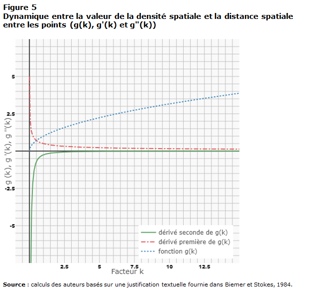Les similitudes entre ${\text{y}}^{\text{'}\text{'}}\left({\text{x}}^{\text{'}\text{'}}\right)$ et $\text{f}\left(\text{x}\right)$ sont pertinentes pour comprendre le lien théorique de $\text{f}\left(\text{x}\right)$ avec la distribution normale, d'autant plus que la normale était un paramètre optionnel dans Sergerie et al., 2021. La Figure 3 présente les trois courbes d’intérêts pour comprendre l'image complète de $\text{f}\left(\text{x}\right)$ , à savoir la fonction $\text{f}\left(\text{x}\right)$ en bleu, sa fonction de dérivée première en rouge et sa fonction de dérivée seconde en vert. L'axe des $\text{x}$ représente le rapport $\text{x}$ (Bartle et Sherbert, 2011).

Description de la figure 3

Figure 3
Fonction de densité du noyau polynomiale (zoom arrière pour f(x), f'(x) et f''(x))
Sommaire du tableau
Les données sont présentées selon rapport de la distance à la taille de la bande passante (x) (titres de rangée) et , calculées selon (figurant comme en-tête de colonne).

rapport de la distance à la taille de la bande passante (x)	fonction d’intérêt (bleu) f(x)	dérivée première (rouge) f'(x)	dérivée seconde (vert) f''(x)
Source : calculs des auteurs à partir de la fonction d’estimation de la densité du noyau de Parzen (1962) et Rosenblatt (1956). Légende : Bleu = fonction d’intérêt , rouge = dérivée première de , et vert = dérivée seconde de
-2.50	26,32024871	-50,13380707	67,80000576
-2.49	25,8222911	-49,45866799	67,22819388
-2.48	25,33105633	-48,78923556	66,65867383
-2.47	24,84648745	-48,12548687	66,09144561
-2.46	24,36852773	-47,46739901	65,52650923
-2.45	23,89712067	-46,81494905	64,96386467
-2.44	23,43221003	-46,16811407	64,40351195
-2.43	22,97373975	-45,52687117	63,84545106
-2.42	22,52165404	-44,89119741	63,28968199
-2.41	22,07589732	-44,26106989	62,73620476
-2.40	21,63641423	-43,63646568	62,18501936
-2.39	21,20314967	-43,01736186	61,6361258
-2.38	20,77604874	-42,40373552	61,08952406
-2.37	20,35505678	-41,79556374	60,54521416
-2.36	19,94011936	-41,1928236	60,00319608
-2.35	19,53118227	-40,59549218	59,46346984
-2.34	19,12819156	-40,00354656	58,92603543
-2.33	18,73109347	-39,41696383	58,39089285
-2.32	18,33983448	-38,83572107	57,8580421
-2.31	17,95436132	-38,25979535	57,32748318
-2.30	17,57462093	-37,68916376	56,79921609
-2.29	17,20056048	-37,12380339	56,27324083
-2.28	16,83212737	-36,56369131	55,74955741
-2.27	16,46926923	-36,0088046	55,22816582
-2.26	16,11193393	-35,45912035	54,70906605
-2.25	15,76006956	-34,91461564	54,19225812
-2.24	15,41362443	-34,37526755	53,67774202
-2.23	15,0725471	-33,84105316	53,16551775
-2.22	14,73678633	-33,31194956	52,65558532
-2.21	14,40629115	-32,78793382	52,14794471
-2.20	14,08101077	-32,26898302	51,64259593
-2.19	13,76089468	-31,75507426	51,13953899
-2.18	13,44589256	-31,2461846	50,63877388
-2.17	13,13595433	-30,74229114	50,1403006
-2.16	12,83103016	-30,24337095	49,64411915
-2.15	12,53107041	-29,74940112	49,15022953
-2.14	12,23602571	-29,26035872	48,65863174
-2.13	11,94584689	-28,77622084	48,16932578
-2.12	11,66048502	-28,29696457	47,68231165
-2.11	11,3798914	-27,82256697	47,19758936
-2.10	11,10401756	-27,35300514	46,7151589
-2.09	10,83281526	-26,88825615	46,23502026
-2.08	10,56623647	-26,42829709	45,75717346
-2.07	10,30423343	-25,97310504	45,28161849
-2.06	10,04675856	-25,52265709	44,80835535
-2.05	9,793764546	-25,0769303	44,33738405
-2.04	9,545204292	-24,63590177	43,86870457
-2.03	9,301030927	-24,19954857	43,40231692
-2.02	9,061197812	-23,76784779	42,93822111
-2.01	8,825658539	-23,34077651	42,47641713
-2.00	8,594366927	-22,91831181	42,01690498
-1.99	8,367277024	-22,50043077	41,55968466
-1.98	8,144343109	-22,08711047	41,10475617
-1.97	7,925519689	-21,678328	40,65211951
-1.96	7,710761499	-21,27406044	40,20177468
-1.95	7,500023507	-20,87428487	39,75372169
-1.94	7,293260905	-20,47897837	39,30796052
-1.93	7,090429119	-20,08811802	38,86449119
-1.92	6,891483801	-19,70168091	38,42331369
-1.91	6,696380833	-19,31964411	37,98442801
-1.90	6,505076327	-18,94198471	37,54783417
-1.89	6,317526624	-18,56867979	37,11353217
-1.88	6,133688293	-18,19970642	36,68152199
-1.87	5,953518133	-17,83504171	36,25180364
-1.86	5,776973173	-17,47466271	35,82437713
-1.85	5,60401067	-17,11854652	35,39924244
-1.84	5,434588109	-16,76667022	34,97639959
-1.83	5,268663208	-16,41901089	34,55584857
-1.82	5,106193911	-16,07554561	34,13758938
-1.81	4,947138392	-15,73625147	33,72162202
-1.80	4,791455055	-15,40110553	33,30794649
-1.79	4,639102531	-15,0700849	32,89656279
-1.78	4,490039682	-14,74316664	32,48747093
-1.77	4,3442256	-14,42032784	32,08067089
-1.76	4,201619604	-14,10154558	31,67616269
-1.75	4,062181243	-13,78679695	31,27394632
-1.74	3,925870296	-13,47605901	30,87402178
-1.73	3,79264677	-13,16930887	30,47638907
-1.72	3,662470902	-12,86652359	30,08104819
-1.71	3,535303158	-12,56768027	29,68799914
-1.70	3,411104233	-12,27275597	29,29724192
-1.69	3,289835052	-11,98172779	28,90877654
-1.68	3,171456767	-11,6945728	28,52260299
-1.67	3,055930761	-11,41126809	28,13872126
-1.66	2,943218647	-11,13179074	27,75713137
-1.65	2,833282265	-10,85611782	27,37783331
-1.64	2,726083686	-10,58422643	27,00082708
-1.63	2,621585208	-10,31609364	26,62611268
-1.62	2,519749361	-10,05169654	26,25369012
-1.61	2,420538901	-9,7910122	25,88355938
-1.60	2,323916817	-9,534017711	25,51572048
-1.59	2,229846324	-9,280690151	25,1501734
-1.58	2,138290867	-9,031006603	24,78691816
-1.57	2,049214122	-8,784944149	24,42595475
-1.56	1,96257999	-8,542479869	24,06728317
-1.55	1,878352607	-8,303590846	23,71090342
-1.54	1,796496332	-8,068254161	23,3568155
-1.53	1,716975759	-7,836446896	23,00501942
-1.52	1,639755706	-7,608146133	22,65551516
-1.51	1,564801224	-7,383328954	22,30830274
-1.50	1,492077591	-7,161972439	21,96338215
-1.49	1,421550316	-6,944053671	21,62075339
-1.48	1,353185135	-6,729549732	21,28041645
-1.47	1,286948015	-6,518437703	20,94237136
-1.46	1,222805151	-6,310694665	20,60661809
-1.45	1,160722968	-6,106297702	20,27315665
-1.44	1,10066812	-5,905223893	19,94198705
-1.43	1,04260749	-5,707450321	19,61310927
-1.42	0,986508189	-5,512954068	19,28652333
-1.41	0,93233756	-5,321712215	18,96222922
-1.40	0,880063173	-5,133701844	18,64022693
-1.39	0,829652828	-4,948900037	18,32051649
-1.38	0,781074554	-4,767283875	18,00309787
-1.37	0,734296608	-4,58883044	17,68797108
-1.36	0,689287479	-4,413516814	17,37513612
-1.35	0,646015882	-4,241320078	17,064593
-1.34	0,604450764	-4,072217315	16,7563417
-1.33	0,564561299	-3,906185605	16,45038224
-1.32	0,526316892	-3,743202031	16,14671461
-1.31	0,489687175	-3,583243673	15,84533881
-1.30	0,45464201	-3,426287615	15,54625484
-1.29	0,421151491	-3,272310937	15,2494627
-1.28	0,389185937	-3,121290721	14,9549624
-1.27	0,358715898	-2,97320405	14,66275392
-1.26	0,329712154	-2,828028004	14,37283728
-1.25	0,302145712	-2,685739665	14,08521246
-1.24	0,275987811	-2,546316115	13,79987948
-1.23	0,251209917	-2,409734436	13,51683833
-1.22	0,227783726	-2,275971709	13,23608901
-1.21	0,205681163	-2,145005016	12,95763152
-1.20	0,184874382	-2,016811439	12,68146587
-1.19	0,165335767	-1,891368059	12,40759204
-1.18	0,14703793	-1,768651959	12,13601004
-1.17	0,129953713	-1,648640219	11,86671988
-1.16	0,114056187	-1,531309922	11,59972155
-1.15	0,099318653	-1,416638148	11,33501505
-1.14	0,085714639	-1,304601981	11,07260038
-1.13	0,073217904	-1,195178501	10,81247754
-1.12	0,061802436	-1,088344791	10,55464653
-1.11	0,051442452	-0,984077931	10,29910735
-1.10	0,042112398	-0,882355005	10,04586001
-1.09	0,033786949	-0,783153092	9,794904494
-1.08	0,026441009	-0,686449275	9,546240811
-1.07	0,020049713	-0,592220636	9,299868959
-1.06	0,014588422	-0,500444257	9,055788938
-1.05	0,01003273	-0,411097218	8,814000748
-1.04	0,006358456	-0,324156602	8,57450439
-1.03	0,003541653	-0,239599491	8,337299863
-1.02	0,001558598	-0,157402965	8,102387167
-1.01	0,000385801	-0,077544108	7,869766302
-1.00	0	-7,4607E-14	7,639437268
-0.99	0,000378162	0,075252277	7,411400066
-0.98	0,001497482	0,148235641	7,185654695
-0.97	0,003335388	0,21897301	6,962201155
-0.96	0,005869532	0,287487303	6,741039446
-0.95	0,0090778	0,353801438	6,522169568
-0.94	0,012938304	0,417938334	6,305591521
-0.93	0,017429386	0,479920908	6,091305306
-0.92	0,022529617	0,53977208	5,879310922
-0.91	0,028217799	0,597514766	5,669608369
-0.90	0,034472961	0,653171886	5,462197647
-0.89	0,041274361	0,706766359	5,257078756
-0.88	0,048601489	0,758321101	5,054251697
-0.87	0,056434061	0,807859032	4,853716468
-0.86	0,064752023	0,85540307	4,655473071
-0.85	0,073535552	0,900976133	4,459521505
-0.84	0,082765052	0,944601139	4,265861771
-0.83	0,092421158	0,986301008	4,074493867
-0.82	0,102484732	1,026098656	3,885417795
-0.81	0,112936866	1,064017003	3,698633554
-0.80	0,123758884	1,100078967	3,514141143
-0.79	0,134932334	1,134307465	3,331940565
-0.78	0,146438998	1,166725417	3,152031817
-0.77	0,158260884	1,197355741	2,9744149
-0.76	0,17038023	1,226221355	2,799089815
-0.75	0,182779505	1,253345177	2,626056561
-0.74	0,195441404	1,278750125	2,455315138
-0.73	0,208348854	1,302459119	2,286865546
-0.72	0,22148501	1,324495076	2,120707786
-0.71	0,234833255	1,344880914	1,956841856
-0.70	0,248377204	1,363639552	1,795267758
-0.69	0,262100699	1,380793909	1,635985491
-0.68	0,275987811	1,396366902	1,478995055
-0.67	0,290022842	1,410381449	1,32429645
-0.66	0,304190322	1,42286047	1,171889677
-0.65	0,318475009	1,433826882	1,021774735
-0.64	0,332861894	1,443303604	0,873951624
-0.63	0,347336192	1,451313554	0,728420344
-0.62	0,361883352	1,457879651	0,585180895
-0.61	0,376489049	1,463024812	0,444233277
-0.60	0,391139188	1,466771956	0,305577491
-0.59	0,405819904	1,469144001	0,169213535
-0.58	0,420517561	1,470163866	0,035141411
-0.57	0,435218751	1,469854468	-0,096638881
-0.56	0,449910296	1,468238727	-0,226127343
-0.55	0,464579247	1,465339561	-0,353323974
-0.54	0,479212885	1,461179887	-0,478228773
-0.53	0,49379872	1,455782625	-0,600841741
-0.52	0,508324489	1,449170692	-0,721162878
-0.51	0,522778161	1,441367007	-0,839192184
-0.50	0,537147933	1,432394488	-0,954929659
-0.49	0,551422231	1,422276053	-1,068375302
-0.48	0,565589711	1,411034621	-1,179529114
-0.47	0,579639257	1,39869311	-1,288391095
-0.46	0,593559982	1,385274439	-1,394961245
-0.45	0,607341231	1,370801525	-1,499239564
-0.44	0,620972575	1,355297287	-1,601226051
-0.43	0,634443816	1,338784643	-1,700920708
-0.42	0,647744983	1,321286512	-1,798323533
-0.41	0,660866337	1,302825812	-1,893434527
-0.40	0,673798367	1,283425461	-1,98625369
-0.39	0,686531791	1,263108378	-2,076781021
-0.38	0,699057555	1,24189748	-2,165016522
-0.37	0,711366837	1,219815687	-2,250960191
-0.36	0,723451042	1,196885916	-2,334612029
-0.35	0,735301805	1,173131086	-2,415972036
-0.34	0,74691099	1,148574114	-2,495040212
-0.33	0,75827069	1,123237921	-2,571816556
-0.32	0,769373228	1,097145423	-2,64630107
-0.31	0,780211154	1,070319539	-2,718493752
-0.30	0,79077725	1,042783187	-2,788394603
-0.29	0,801064526	1,014559286	-2,856003623
-0.28	0,811066221	0,985670754	-2,921320811
-0.27	0,820775802	0,956140509	-2,984346169
-0.26	0,830186968	0,92599147	-3,045079695
-0.25	0,839293645	0,895246555	-3,10352139
-0.24	0,848089989	0,863928682	-3,159671254
-0.23	0,856570385	0,832060769	-3,213529287
-0.22	0,864729448	0,799665736	-3,265095489
-0.21	0,872562019	0,766766499	-3,314369859
-0.20	0,880063173	0,733385978	-3,361352398
-0.19	0,887228211	0,69954709	-3,406043106
-0.18	0,894052664	0,665272755	-3,448441983
-0.17	0,900532291	0,63058589	-3,488549029
-0.16	0,906663083	0,595509414	-3,526364243
-0.15	0,912441257	0,560066245	-3,561887626
-0.14	0,917863262	0,524279301	-3,595119179
-0.13	0,922925774	0,488171501	-3,626058899
-0.12	0,927625699	0,451765762	-3,654706789
-0.11	0,931960172	0,415085004	-3,681062848
-0.10	0,935926558	0,378152145	-3,705127075
-0.09	0,939522451	0,340990102	-3,726899471
-0.08	0,942745673	0,303621795	-3,746380036
-0.07	0,945594276	0,266070141	-3,76356877
-0.06	0,948066541	0,228358059	-3,778465673
-0.05	0,950160979	0,190508467	-3,791070744
-0.04	0,951876328	0,152544283	-3,801383985
-0.03	0,953211559	0,114488427	-3,809405394
-0.02	0,954165868	0,076363815	-3,815134972
-0.01	0,954738682	0,038193367	-3,818572719
0.00	0,954929659	3,44428E-14	-3,819718634
0.01	0,954738682	-0,038193367	-3,818572719
0.02	0,954165868	-0,076363815	-3,815134972
0.03	0,953211559	-0,114488427	-3,809405394
0.04	0,951876328	-0,152544283	-3,801383985
0.05	0,950160979	-0,190508467	-3,791070744
0.06	0,948066541	-0,228358059	-3,778465673
0.07	0,945594276	-0,266070141	-3,76356877
0.08	0,942745673	-0,303621795	-3,746380036
0.09	0,939522451	-0,340990102	-3,726899471
0.10	0,935926558	-0,378152145	-3,705127075
0.11	0,931960172	-0,415085004	-3,681062848
0.12	0,927625699	-0,451765762	-3,654706789
0.13	0,922925774	-0,488171501	-3,626058899
0.14	0,917863262	-0,524279301	-3,595119179
0.15	0,912441257	-0,560066245	-3,561887626
0.16	0,906663083	-0,595509414	-3,526364243
0.17	0,900532291	-0,63058589	-3,488549029
0.18	0,894052664	-0,665272755	-3,448441983
0.19	0,887228211	-0,69954709	-3,406043106
0.20	0,880063173	-0,733385978	-3,361352398
0.21	0,872562019	-0,766766499	-3,314369859
0.22	0,864729448	-0,799665736	-3,265095489
0.23	0,856570385	-0,832060769	-3,213529287
0.24	0,848089989	-0,863928682	-3,159671254
0.25	0,839293645	-0,895246555	-3,10352139
0.26	0,830186968	-0,92599147	-3,045079695
0.27	0,820775802	-0,956140509	-2,984346169
0.28	0,811066221	-0,985670754	-2,921320811
0.29	0,801064526	-1,014559286	-2,856003623
0.30	0,79077725	-1,042783187	-2,788394603
0.31	0,780211154	-1,070319539	-2,718493752
0.32	0,769373228	-1,097145423	-2,64630107
0.33	0,75827069	-1,123237921	-2,571816556
0.34	0,74691099	-1,148574114	-2,495040212
0.35	0,735301805	-1,173131086	-2,415972036
0.36	0,723451042	-1,196885916	-2,334612029
0.37	0,711366837	-1,219815687	-2,250960191
0.38	0,699057555	-1,24189748	-2,165016522
0.39	0,686531791	-1,263108378	-2,076781021
0.40	0,673798367	-1,283425461	-1,98625369
0.41	0,660866337	-1,302825812	-1,893434527
0.42	0,647744983	-1,321286512	-1,798323533
0.43	0,634443816	-1,338784643	-1,700920708
0.44	0,620972575	-1,355297287	-1,601226051
0.45	0,607341231	-1,370801525	-1,499239564
0.46	0,593559982	-1,385274439	-1,394961245
0.47	0,579639257	-1,39869311	-1,288391095
0.48	0,565589711	-1,411034621	-1,179529114
0.49	0,551422231	-1,422276053	-1,068375302
0.50	0,537147933	-1,432394488	-0,954929659
0.51	0,522778161	-1,441367007	-0,839192184
0.52	0,508324489	-1,449170692	-0,721162878
0.53	0,49379872	-1,455782625	-0,600841741
0.54	0,479212885	-1,461179887	-0,478228773
0.55	0,464579247	-1,465339561	-0,353323974
0.56	0,449910296	-1,468238727	-0,226127343
0.57	0,435218751	-1,469854468	-0,096638881
0.58	0,420517561	-1,470163866	0,035141411
0.59	0,405819904	-1,469144001	0,169213535
0.60	0,391139188	-1,466771956	0,305577491
0.61	0,376489049	-1,463024812	0,444233277
0.62	0,361883352	-1,457879651	0,585180895
0.63	0,347336192	-1,451313554	0,728420344
0.64	0,332861894	-1,443303604	0,873951624
0.65	0,318475009	-1,433826882	1,021774735
0.66	0,304190322	-1,42286047	1,171889677
0.67	0,290022842	-1,410381449	1,32429645
0.68	0,275987811	-1,396366902	1,478995055
0.69	0,262100699	-1,380793909	1,635985491
0.70	0,248377204	-1,363639552	1,795267758
0.71	0,234833255	-1,344880914	1,956841856
0.72	0,22148501	-1,324495076	2,120707786
0.73	0,208348854	-1,302459119	2,286865546
0.74	0,195441404	-1,278750125	2,455315138
0.75	0,182779505	-1,253345177	2,626056561
0.76	0,17038023	-1,226221355	2,799089815
0.77	0,158260884	-1,197355741	2,9744149
0.78	0,146438998	-1,166725417	3,152031817
0.79	0,134932334	-1,134307465	3,331940565
0.80	0,123758884	-1,100078967	3,514141143
0.81	0,112936866	-1,064017003	3,698633554
0.82	0,102484732	-1,026098656	3,885417795
0.83	0,092421158	-0,986301008	4,074493867
0.84	0,082765052	-0,944601139	4,265861771
0.85	0,073535552	-0,900976133	4,459521505
0.86	0,064752023	-0,85540307	4,655473071
0.87	0,056434061	-0,807859032	4,853716468
0.88	0,048601489	-0,758321101	5,054251697
0.89	0,041274361	-0,706766359	5,257078756
0.90	0,034472961	-0,653171886	5,462197647
0.91	0,028217799	-0,597514766	5,669608369
0.92	0,022529617	-0,53977208	5,879310922
0.93	0,017429386	-0,479920908	6,091305306
0.94	0,012938304	-0,417938334	6,305591521
0.95	0,0090778	-0,353801438	6,522169568
0.96	0,005869532	-0,287487303	6,741039446
0.97	0,003335388	-0,21897301	6,962201155
0.98	0,001497482	-0,148235641	7,185654695
0.99	0,000378162	-0,075252277	7,411400066
1.00	0	-6,35048E-14	7,639437268
1.01	0,000385801	0,077544108	7,869766302
1.02	0,001558598	0,157402965	8,102387167
1.03	0,003541653	0,239599491	8,337299863
1.04	0,006358456	0,324156602	8,57450439
1.05	0,01003273	0,411097218	8,814000748
1.06	0,014588422	0,500444257	9,055788938
1.07	0,020049713	0,592220636	9,299868959
1.08	0,026441009	0,686449275	9,546240811
1.09	0,033786949	0,783153092	9,794904494
1.10	0,042112398	0,882355005	10,04586001
1.11	0,051442452	0,984077931	10,29910735
1.12	0,061802436	1,088344791	10,55464653
1.13	0,073217904	1,195178501	10,81247754
1.14	0,085714639	1,304601981	11,07260038
1.15	0,099318653	1,416638148	11,33501505
1.16	0,114056187	1,531309922	11,59972155
1.17	0,129953713	1,648640219	11,86671988
1.18	0,14703793	1,768651959	12,13601004
1.19	0,165335767	1,891368059	12,40759204
1.20	0,184874382	2,016811439	12,68146587
1.21	0,205681163	2,145005016	12,95763152
1.22	0,227783726	2,275971709	13,23608901
1.23	0,251209917	2,409734436	13,51683833
1.24	0,275987811	2,546316115	13,79987948
1.25	0,302145712	2,685739665	14,08521246
1.26	0,329712154	2,828028004	14,37283728
1.27	0,358715898	2,97320405	14,66275392
1.28	0,389185937	3,121290721	14,9549624
1.29	0,421151491	3,272310937	15,2494627
1.30	0,45464201	3,426287615	15,54625484
1.31	0,489687175	3,583243673	15,84533881
1.32	0,526316892	3,743202031	16,14671461
1.33	0,564561299	3,906185605	16,45038224
1.34	0,604450764	4,072217315	16,7563417
1.35	0,646015882	4,241320078	17,064593
1.36	0,689287479	4,413516814	17,37513612
1.37	0,734296608	4,58883044	17,68797108
1.38	0,781074554	4,767283875	18,00309787
1.39	0,829652828	4,948900037	18,32051649
1.40	0,880063173	5,133701844	18,64022693
1.41	0,93233756	5,321712215	18,96222922
1.42	0,986508189	5,512954068	19,28652333
1.43	1,04260749	5,707450321	19,61310927
1.44	1,10066812	5,905223893	19,94198705
1.45	1,160722968	6,106297702	20,27315665
1.46	1,222805151	6,310694665	20,60661809
1.47	1,286948015	6,518437703	20,94237136
1.48	1,353185135	6,729549732	21,28041645
1.49	1,421550316	6,944053671	21,62075339
1.50	1,492077591	7,161972439	21,96338215
1.51	1,564801224	7,383328954	22,30830274
1.52	1,639755706	7,608146133	22,65551516
1.53	1,716975759	7,836446896	23,00501942
1.54	1,796496332	8,068254161	23,3568155
1.55	1,878352607	8,303590846	23,71090342
1.56	1,96257999	8,542479869	24,06728317
1.57	2,049214122	8,784944149	24,42595475
1.58	2,138290867	9,031006603	24,78691816
1.59	2,229846324	9,280690151	25,1501734
1.60	2,323916817	9,534017711	25,51572048
1.61	2,420538901	9,7910122	25,88355938
1.62	2,519749361	10,05169654	26,25369012
1.63	2,621585208	10,31609364	26,62611268
1.64	2,726083686	10,58422643	27,00082708
1.65	2,833282265	10,85611782	27,37783331
1.66	2,943218647	11,13179074	27,75713137
1.67	3,055930761	11,41126809	28,13872126
1.68	3,171456767	11,6945728	28,52260299
1.69	3,289835052	11,98172779	28,90877654
1.70	3,411104233	12,27275597	29,29724192
1.71	3,535303158	12,56768027	29,68799914
1.72	3,662470902	12,86652359	30,08104819
1.73	3,79264677	13,16930887	30,47638907
1.74	3,925870296	13,47605901	30,87402178
1.75	4,062181243	13,78679695	31,27394632
1.76	4,201619604	14,10154558	31,67616269
1.77	4,3442256	14,42032784	32,08067089
1.78	4,490039682	14,74316664	32,48747093
1.79	4,639102531	15,0700849	32,89656279
1.80	4,791455055	15,40110553	33,30794649
1.81	4,947138392	15,73625147	33,72162202
1.82	5,106193911	16,07554561	34,13758938
1.83	5,268663208	16,41901089	34,55584857
1.84	5,434588109	16,76667022	34,97639959
1.85	5,60401067	17,11854652	35,39924244
1.86	5,776973173	17,47466271	35,82437713
1.87	5,953518133	17,83504171	36,25180364
1.88	6,133688293	18,19970642	36,68152199
1.89	6,317526624	18,56867979	37,11353217
1.90	6,505076327	18,94198471	37,54783417
1.91	6,696380833	19,31964411	37,98442801
1.92	6,891483801	19,70168091	38,42331369
1.93	7,090429119	20,08811802	38,86449119
1.94	7,293260905	20,47897837	39,30796052
1.95	7,500023507	20,87428487	39,75372169
1.96	7,710761499	21,27406044	40,20177468
1.97	7,925519689	21,678328	40,65211951
1.98	8,144343109	22,08711047	41,10475617
1.99	8,367277024	22,50043077	41,55968466
2.00	8,594366927	22,91831181	42,01690498
2.01	8,825658539	23,34077651	42,47641713
2.02	9,061197812	23,76784779	42,93822111
2.03	9,301030927	24,19954857	43,40231692
2.04	9,545204292	24,63590177	43,86870457
2.05	9,793764546	25,0769303	44,33738405
2.06	10,04675856	25,52265709	44,80835535
2.07	10,30423343	25,97310504	45,28161849
2.08	10,56623647	26,42829709	45,75717346
2.09	10,83281526	26,88825615	46,23502026
2.10	11,10401756	27,35300514	46,7151589
2.11	11,3798914	27,82256697	47,19758936
2.12	11,66048502	28,29696457	47,68231165
2.13	11,94584689	28,77622084	48,16932578
2.14	12,23602571	29,26035872	48,65863174
2.15	12,53107041	29,74940112	49,15022953
2.16	12,83103016	30,24337095	49,64411915
2.17	13,13595433	30,74229114	50,1403006
2.18	13,44589256	31,2461846	50,63877388
2.19	13,76089468	31,75507426	51,13953899
2.20	14,08101077	32,26898302	51,64259593
2.21	14,40629115	32,78793382	52,14794471
2.22	14,73678633	33,31194956	52,65558532
2.23	15,0725471	33,84105316	53,16551775
2.24	15,41362443	34,37526755	53,67774202
2.25	15,76006956	34,91461564	54,19225812
2.26	16,11193393	35,45912035	54,70906605
2.27	16,46926923	36,0088046	55,22816582
2.28	16,83212737	36,56369131	55,74955741
2.29	17,20056048	37,12380339	56,27324083
2.30	17,57462093	37,68916376	56,79921609
2.31	17,95436132	38,25979535	57,32748318
2.32	18,33983448	38,83572107	57,8580421
2.33	18,73109347	39,41696383	58,39089285
2.34	19,12819156	40,00354656	58,92603543
2.35	19,53118227	40,59549218	59,46346984
2.36	19,94011936	41,1928236	60,00319608
2.37	20,35505678	41,79556374	60,54521416
2.38	20,77604874	42,40373552	61,08952406
2.39	21,20314967	43,01736186	61,6361258
2.40	21,63641423	43,63646568	62,18501936
2.41	22,07589732	44,26106989	62,73620476
2.42	22,52165404	44,89119741	63,28968199
2.43	22,97373975	45,52687117	63,84545106
2.44	23,43221003	46,16811407	64,40351195
2.45	23,89712067	46,81494905	64,96386467
2.46	24,36852773	47,46739901	65,52650923
2.47	24,84648745	48,12548687	66,09144561
2.48	25,33105633	48,78923556	66,65867383
2.49	25,8222911	49,45866799	67,22819388
2.50	26,32024871	50,13380707	67,80000576

Maintenant que la fonction de densité du noyau polynomiale est bien décrite mathématiquement, nous nous concentrons sur le sous-domaine pertinent de la fonction $\text{f}\left(\text{x}\right)$ qui est $[0,1]$ et non $(-\text{∞},+\text{∞})$ . En effet, le rapport $\text{x}$ n’a aucune utilité en dessous de zéro ni au-delà de 1 dans le contexte d’un exercice d’estimation de la densité, car $\text{Θ}$ ne peut pas être inférieur à zéro (c’est-à-dire qu’une distance négative du point d’intérêt spatial n’est pas pertinente) et ne peut pas dépasser $\text{ψ}$ (dépasser la zone circulaire ciblée n’est également pas pertinent). Par conséquent, l’image pertinente de $\text{f}\left(\text{x}\right)$ est $[\text{0,}\frac{3}{\text{π}}]$, parce que $\text{f (0) = }\frac{3}{\text{π}}$ et $\text{f (1) = 0}$, et $\text{f}$ est une fonction décroissante entre 0 et 1. Plus important encore, la contribution distincte d’un emplacement d’emploi  $\text{i}$ dans le rayon ciblé $\text{ψ}$ est approximativement normalisé entre 0 et 1 [c’est-à-dire entre les valeurs 0 et $\left(3/3,14159\right)=0,95)$]. De plus, $\text{PKDF()}$ est une somme finie de termes approximativement normalisés puisque le nombre de lieux des emplois dans l’environnement circulaire et symétrique $\text{π}{\text{ψ}}^2$ est fini. La Figure 4 est identique à la Figure 3 précédente. Cependant, elle se concentre sur le domaine et l'image pertinents de $\text{f}\left(\text{x}\right)$ et permet donc de mieux visualiser la valeur de $\text{f}\left(\text{x}\right)$ lorsque $\text{x}=0$, qui n'est pas 1, mais 0,95. La contribution du lieu de travail $\text{i}$ diminue lorsque $\text{x}$ augmente entre $[0,+1]$. La diminution est initialement moins forte autour de zéro, mais devient ensuite plus marquée puis moins forte une fois de plus juste avant d'atteindre un rapport $\text{x}$ égal à 1. Cette structure est due au fait que la dérivée seconde (courbe verte) atteint une valeur nulle lorsque $\text{x}$ atteint +0,577. Un carré surligné en jaune délimite la région d'intérêt (Bartle et Sherbert, 2011).     

Description de la figure 4

Figure 4
Fonction de densité du noyau polynomiale (zoom avant pour le domaine [0,1] de f(x), f'(x) et f''(x)) Sommaire du tableau
Les données sont présentées selon rapport de la distance à la taille de la bande passante (x) (titres de rangée) et , calculées selon (figurant comme en-tête de colonne).

rapport de la distance à la taille de la bande passante (x)	fonction d’intérêt (bleu) f(x)	dérivée première (rouge) f'(x)	dérivée seconde (vert) f''(x)
Source : calculs des auteurs à partir de la fonction d’estimation de la densité du noyau de Parzen (1962) et Rosenblatt (1956). Légende : Bleu = fonction d’intérêt , rouge = dérivée première de , et vert = dérivée seconde de
0.00	0,954929659	0	-3,819718634
0.01	0,954738682	-0,038193367	-3,818572719
0.02	0,954165868	-0,076363815	-3,815134972
0.03	0,953211559	-0,114488427	-3,809405394
0.04	0,951876328	-0,152544283	-3,801383985
0.05	0,950160979	-0,190508467	-3,791070744
0.06	0,948066541	-0,228358059	-3,778465673
0.07	0,945594276	-0,266070141	-3,76356877
0.08	0,942745673	-0,303621795	-3,746380036
0.09	0,939522451	-0,340990102	-3,726899471
0.10	0,935926558	-0,378152145	-3,705127075
0.11	0,931960172	-0,415085004	-3,681062848
0.12	0,927625699	-0,451765762	-3,654706789
0.13	0,922925774	-0,488171501	-3,626058899
0.14	0,917863262	-0,524279301	-3,595119179
0.15	0,912441257	-0,560066245	-3,561887626
0.16	0,906663083	-0,595509414	-3,526364243
0.17	0,900532291	-0,63058589	-3,488549029
0.18	0,894052664	-0,665272755	-3,448441983
0.19	0,887228211	-0,69954709	-3,406043106
0.20	0,880063173	-0,733385978	-3,361352398
0.21	0,872562019	-0,766766499	-3,314369859
0.22	0,864729448	-0,799665736	-3,265095489
0.23	0,856570385	-0,832060769	-3,213529287
0.24	0,848089989	-0,863928682	-3,159671254
0.25	0,839293645	-0,895246555	-3,10352139
0.26	0,830186968	-0,92599147	-3,045079695
0.27	0,820775802	-0,956140509	-2,984346169
0.28	0,811066221	-0,985670754	-2,921320811
0.29	0,801064526	-1,014559286	-2,856003623
0.30	0,79077725	-1,042783187	-2,788394603
0.31	0,780211154	-1,070319539	-2,718493752
0.32	0,769373228	-1,097145423	-2,64630107
0.33	0,75827069	-1,123237921	-2,571816556
0.34	0,74691099	-1,148574114	-2,495040212
0.35	0,735301805	-1,173131086	-2,415972036
0.36	0,723451042	-1,196885916	-2,334612029
0.37	0,711366837	-1,219815687	-2,250960191
0.38	0,699057555	-1,24189748	-2,165016522
0.39	0,686531791	-1,263108378	-2,076781021
0.40	0,673798367	-1,283425461	-1,98625369
0.41	0,660866337	-1,302825812	-1,893434527
0.42	0,647744983	-1,321286512	-1,798323533
0.43	0,634443816	-1,338784643	-1,700920708
0.44	0,620972575	-1,355297287	-1,601226051
0.45	0,607341231	-1,370801525	-1,499239564
0.46	0,593559982	-1,385274439	-1,394961245
0.47	0,579639257	-1,39869311	-1,288391095
0.48	0,565589711	-1,411034621	-1,179529114
0.49	0,551422231	-1,422276053	-1,068375302
0.50	0,537147933	-1,432394488	-0,954929659
0.51	0,522778161	-1,441367007	-0,839192184
0.52	0,508324489	-1,449170692	-0,721162878
0.53	0,49379872	-1,455782625	-0,600841741
0.54	0,479212885	-1,461179887	-0,478228773
0.55	0,464579247	-1,465339561	-0,353323974
0.56	0,449910296	-1,468238727	-0,226127343
0.57	0,435218751	-1,469854468	-0,096638881
0.58	0,420517561	-1,470163866	0,035141411
0.59	0,405819904	-1,469144001	0,169213535
0.60	0,391139188	-1,466771956	0,305577491
0.61	0,376489049	-1,463024812	0,444233277
0.62	0,361883352	-1,457879651	0,585180895
0.63	0,347336192	-1,451313554	0,728420344
0.64	0,332861894	-1,443303604	0,873951624
0.65	0,318475009	-1,433826882	1,021774735
0.66	0,304190322	-1,42286047	1,171889677
0.67	0,290022842	-1,410381449	1,32429645
0.68	0,275987811	-1,396366902	1,478995055
0.69	0,262100699	-1,380793909	1,635985491
0.70	0,248377204	-1,363639552	1,795267758
0.71	0,234833255	-1,344880914	1,956841856
0.72	0,22148501	-1,324495076	2,120707786
0.73	0,208348854	-1,302459119	2,286865546
0.74	0,195441404	-1,278750125	2,455315138
0.75	0,182779505	-1,253345177	2,626056561
0.76	0,17038023	-1,226221355	2,799089815
0.77	0,158260884	-1,197355741	2,9744149
0.78	0,146438998	-1,166725417	3,152031817
0.79	0,134932334	-1,134307465	3,331940565
0.80	0,123758884	-1,100078967	3,514141143
0.81	0,112936866	-1,064017003	3,698633554
0.82	0,102484732	-1,026098656	3,885417795
0.83	0,092421158	-0,986301008	4,074493867
0.84	0,082765052	-0,944601139	4,265861771
0.85	0,073535552	-0,900976133	4,459521505
0.86	0,064752023	-0,85540307	4,655473071
0.87	0,056434061	-0,807859032	4,853716468
0.88	0,048601489	-0,758321101	5,054251697
0.89	0,041274361	-0,706766359	5,257078756
0.90	0,034472961	-0,653171886	5,462197647
0.91	0,028217799	-0,597514766	5,669608369
0.92	0,022529617	-0,53977208	5,879310922
0.93	0,017429386	-0,479920908	6,091305306
0.94	0,012938304	-0,417938334	6,305591521
0.95	0,0090778	-0,353801438	6,522169568
0.96	0,005869532	-0,287487303	6,741039446
0.97	0,003335388	-0,21897301	6,962201155
0.98	0,001497482	-0,148235641	7,185654695
0.99	0,000378162	-0,075252277	7,411400066
1.00	0	4,88498E-15	7,639437268

Connexion spatiale entre notre étude et Sergerie et al. (2021)

Avant de passer à la dernière partie de la méthodologie principale de cet article où les étapes de traitement de données sont effectuées sur la base de la distribution de densité du noyau estimée pour les RMR et les SCIAN d'intérêt, nous fournissons rapidement une explication intuitive de la dynamique entre la densité spatiale des emplacements d'emploi et la distance spatiale des emplacements d'emploi. Cette explication est essentielle pour bien comprendre la nature même de nos données et ses limites. Cette explication fournit également des liens entre notre étude et Sergerie et al. (2021) en termes de cartographie spatiale. Un article du Bureau du recensement des États-Unis (Biemer et Stokes, 1984), souligne la phrase suivante : « Justification : La distance moyenne entre des points répartis aléatoirement dans un plan est augmentée de ${\text{k}}^{1/2}$ lorsque la densité de ces points est diminuée d’un facteur $\text{k}$». Cette explication est simple et intuitive, cependant, pour mieux comprendre leur idée, nous générons la fonction $\text{g}\left(\text{k}\right)={\text{ k}}^{1/2}$ et effectuons une étude rapide de ses propriétés de dérivées premières et secondes, de son domaine et de son image. Dans la Figure 5, l'axe horizontal est l'axe $\text{k}$ et un nombre positif $\text{k}$ représente le facteur de diminution de la densité spatiale. La courbe bleue est la fonction $\text{g}\left(\text{k}\right)={\text{ k}}^{1/2}$ et elle représente l'augmentation de la distance moyenne entre les points spatiaux. Le domaine et l'image de la fonction $\text{g}\left(\text{k}\right)={\text{ k}}^{1/2}$ sont l'ensemble des nombres réels non négatifs ${\text{R}}^{+}$ . En d’autres mots, $\text{k}$ et ${\text{k}}^{-\raisebox{1ex}{$1$}\!\left/ \!\raisebox{-1ex}{$2$}\right.}\in \left[0,+\text{∞}\right)$. La courbe rouge est la première dérivée ${\text{g}}^{\text{'}}\left(\text{k}\right)=\frac{\text{d}}{\text{d}\text{k}}{\text{k}}^{\frac{1}{2}}$ et elle est égale à $\frac{1}{2}{\text{*k}}^{-\frac{1}{2}}$ et il n'y a pas de valeur de $\text{k}$ telle qu'elle soit égale à zéro même si elle converge vers zéro, à mesure que  tend vers l’infinie $\left(\frac{1}{2}{\text{*k}}^{-\frac{1}{2}}\to 0\right)$. Son domaine et son image sont tous deux $\left(0,+\text{∞}\right)$ car aucun zéro ne peut être au dénominateur. La courbe verte est la dérivée seconde ${\text{g}}^{\text{'}\text{'}}\left(\text{k}\right)=\frac{{\text{d}}^2}{{\text{dk}}^2}{\text{k}}^{1/2}$ et elle est égale à $-\frac{1}{4}{\text{*k}}^{-\frac{3}{2}}$ et encore une fois, il n'y a pas de valeur de $\text{k}$ telle qu'elle soit égale à zéro même si elle converge vers zéro, à mesure que $\text{k}$ tend vers l’infinie $\left(-\frac{1}{4}{\text{*k}}^{-\frac{3}{2}}\to 0\right)$, et à un rythme de convergence plus rapide que la fonction dérivée première en raison de la plus grande amplitude absolue des paramètres au dénominateur (${\text{g}}^{\text{'}}\left(\text{k}\right)=O\left({\text{k}}^{-\frac{1}{2}}\right),{\text{ g}}^{\text{'}\text{'}}\left(\text{k}\right)=O\left({\text{k}}^{-3/2}\right)$ , et ${\text{k}}^{\frac{1}{2}}<{\text{ k}}^{3/2}\iff 1/{\text{k}}^{3/2}<1/{\text{k}}^{\frac{1}{2}}$ ). Son domaine et son image sont respectivement $\left(0,+\text{∞}\right)$ et $\left(-\text{∞},0\right)$ (Bartle et Sherbert, 2011). Par conséquent, nous expliquons la justification de (Biemer et Stokes, 1984) de la manière suivante pour nos propres applications concernant une grande population de lieux de travail répartis spatialement au sein d'une population d’ID dans une RMR: pour un nombre grand et fixe d'emplacements d'emploi uniformes dans l’ID d'une RMR, alors que les frontières du polygone de l’ID tendent vers l'infini $(\text{DBP } \to \text{∞})$, et que la densité spatiale des emplacements d'emploi tend vers l'infini dans l’ID $\text{(k }\to \text{∞})$ ^Note , et que la distance spatiale moyenne entre les lieux de travail tend vers infiniment (${\text{k}}^{1/2}\to \text{∞}$ ), >et que l'uniformité spatiale aléatoire de l'emplacement du travail est préservé dans l’ID, la variation de la distance spatiale moyenne entre l'emplacement du travail converge en probabilité vers 0 entre les incréments. Dans un context finit, pour 2 expansions larges et distinctes, $\text{k}$ et $\text{k}+\text{Δ}$, avec $\text{Δ}>0$, et chaque expansion est implémentée indépendamment à partir des frontières initiales du polygone de l'ID, alors ${(\text{k}+\text{Δ})}^{1/2}-{\text{k}}^{1/2}\approx 0$. Les informations fournies dans ce paragraphe établissent un lien théorique entre notre étude et celle de Sergerie et al. (2021). Autrement dit, il s'agit des éléments permettant de comprendre le comportement des données d’un ID si la surface aléatoire s'étendait d’un ID à une aire de diffusion (AD) ou même à une aire de diffusion agrégée (ADA).       

Description de la figure 5

Figure 5
Dynamique entre la valeur de la densité spatiale et la distance spatiale entre les points (g(k), g'(k) et g''(k)) Sommaire du tableau
Les données sont présentées selon facteur de réduction de la densité des points spatiaux uniformes sur un plan (k) (titres de rangée) et , calculées selon (figurant comme en-tête de colonne).

facteur de réduction de la densité des points spatiaux uniformes sur un plan (k)	fonction d’intérêt (bleu) g(k)	dérivée première (rouge) g'(k)	dérivée seconde (vert) g''(k)
Note .. n'ayant pas lieu de figurer Source: calculs des auteurs basés sur une justification textuelle fournie dans Biemer et Stokes, 1984. Légende : Bleu = fonction d’intérêt $\text{g(k)}$, rouge = dérivée première de $\text{g(k)}$, et vert = dérivée seconde de $\text{g(k)}$
0.00	0	... n'ayant pas lieu de figurer	... n'ayant pas lieu de figurer
0.01	0,1	5	-250
0.02	0,141421356	3,535533906	-88,38834765
0.03	0,173205081	2,886751346	-48,11252243
0.04	0,2	2,5	-31,25
0.05	0,223606798	2,236067977	-22,36067977
0.06	0,244948974	2,041241452	-17,01034544
0.07	0,264575131	1,889822365	-13,49873118
0.08	0,282842712	1,767766953	-11,04854346
0.09	0,3	1,666666667	-9,259259259
0.10	0,316227766	1,58113883	-7,90569415
0.11	0,331662479	1,507556723	-6,852530559
0.12	0,346410162	1,443375673	-6,014065304
0.13	0,360555128	1,386750491	-5,333655733
0.14	0,374165739	1,33630621	-4,772522177
0.15	0,387298335	1,290994449	-4,303314829
0.16	0,4	1,25	-3,90625
0.17	0,412310563	1,212678125	-3,566700368
0.18	0,424264069	1,178511302	-3,273642505
0.19	0,435889894	1,147078669	-3,018628077
0.20	0,447213595	1,118033989	-2,795084972
0.21	0,458257569	1,091089451	-2,597832027
0.22	0,469041576	1,066003582	-2,422735413
0.23	0,479583152	1,04257207	-2,266461022
0.24	0,489897949	1,020620726	-2,126293179
0.25	0,5	1	-2
0.26	0,509901951	0,980580676	-1,885732069
0.27	0,519615242	0,962250449	-1,781945275
0.28	0,529150262	0,944911183	-1,687341397
0.29	0,538516481	0,928476691	-1,600821881
0.30	0,547722558	0,912870929	-1,521451549
0.31	0,556776436	0,89802651	-1,448429855
0.32	0,565685425	0,883883476	-1,381067932
0.33	0,574456265	0,87038828	-1,318770121
0.34	0,583095189	0,857492926	-1,261019008
0.35	0,591607978	0,845154255	-1,207363221
0.36	0,6	0,833333333	-1,157407407
0.37	0,608276253	0,821994937	-1,110803968
0.38	0,6164414	0,811107106	-1,067246192
0.39	0,6244998	0,800640769	-1,026462524
0.40	0,632455532	0,790569415	-0,988211769
0.41	0,640312424	0,780868809	-0,952279036
0.42	0,64807407	0,77151675	-0,918472321
0.43	0,655743852	0,762492852	-0,886619595
0.44	0,663324958	0,753778361	-0,85656632
0.45	0,670820393	0,745355992	-0,828173325
0.46	0,678232998	0,737209781	-0,801314979
0.47	0,68556546	0,729324957	-0,775877614
0.48	0,692820323	0,721687836	-0,751758163
0.49	0,7	0,714285714	-0,728862974
0.50	0,707106781	0,707106781	-0,707106781
0.51	0,714142843	0,700140042	-0,686411806
0.52	0,721110255	0,693375245	-0,666706967
0.53	0,728010989	0,68680282	-0,647927188
0.54	0,734846923	0,680413817	-0,630012794
0.55	0,741619849	0,674199862	-0,612908966
0.56	0,748331477	0,668153105	-0,596565272
0.57	0,754983444	0,662266179	-0,580935244
0.58	0,761577311	0,656532164	-0,565976004
0.59	0,768114575	0,650944555	-0,551647928
0.60	0,774596669	0,645497224	-0,537914354
0.61	0,781024968	0,6401844	-0,524741311
0.62	0,787400787	0,635000635	-0,512097286
0.63	0,793725393	0,629940788	-0,499953007
0.64	0,8	0,625	-0,48828125
0.65	0,806225775	0,620173673	-0,477056671
0.66	0,81240384	0,615457455	-0,466255648
0.67	0,818535277	0,610847222	-0,455856136
0.68	0,824621125	0,606339063	-0,445837546
0.69	0,830662386	0,601929265	-0,436180627
0.70	0,836660027	0,597614305	-0,42686736
0.71	0,842614977	0,593390829	-0,417880866
0.72	0,848528137	0,589255651	-0,409205313
0.73	0,854400375	0,585205736	-0,400825847
0.74	0,860232527	0,581238194	-0,392728509
0.75	0,866025404	0,577350269	-0,384900179
0.76	0,871779789	0,573539335	-0,37732851
0.77	0,877496439	0,569802882	-0,370001872
0.78	0,883176087	0,566138517	-0,362909306
0.79	0,888819442	0,56254395	-0,356040475
0.80	0,894427191	0,559016994	-0,349385621
0.81	0,9	0,555555556	-0,342935528
0.82	0,905538514	0,55215763	-0,336681482
0.83	0,911043358	0,5488213	-0,330615241
0.84	0,916515139	0,545544726	-0,324729003
0.85	0,921954446	0,542326145	-0,319015379
0.86	0,92736185	0,539163866	-0,313467364
0.87	0,932737905	0,536056267	-0,308078315
0.88	0,938083152	0,533001791	-0,302841927
0.89	0,943398113	0,52999894	-0,297752213
0.90	0,948683298	0,527046277	-0,292803487
0.91	0,953939201	0,524142418	-0,28799034
0.92	0,959166305	0,521286035	-0,283307628
0.93	0,964365076	0,518475847	-0,278750456
0.94	0,969535971	0,515710623	-0,274314161
0.95	0,974679434	0,512989176	-0,269994303
0.96	0,979795897	0,510310363	-0,265786647
0.97	0,98488578	0,507673083	-0,261687156
0.98	0,989949494	0,505076272	-0,257691976
0.99	0,994987437	0,502518908	-0,253797428
1.00	1	0,5	-0,25
1.01	1,004987562	0,497518595	-0,246296334
1.02	1,009950494	0,495073771	-0,242683221
1.03	1,014889157	0,492664639	-0,239157592
1.04	1,019803903	0,490290338	-0,235716509
1.05	1,024695077	0,487950036	-0,23235716
1.06	1,029563014	0,485642931	-0,229076854
1.07	1,034408043	0,483368245	-0,225873011
1.08	1,039230485	0,481125224	-0,222743159
1.09	1,044030651	0,478913143	-0,219684928
1.10	1,048808848	0,476731295	-0,216696043
1.11	1,053565375	0,474578998	-0,213774323
1.12	1,058300524	0,472455591	-0,210917675
1.13	1,063014581	0,470360434	-0,208124086
1.14	1,067707825	0,468292906	-0,205391625
1.15	1,072380529	0,466252404	-0,202718437
1.16	1,077032961	0,464238345	-0,200102735
1.17	1,081665383	0,462250164	-0,197542805
1.18	1,086278049	0,460287309	-0,195036995
1.19	1,090871211	0,458349249	-0,192583718
1.20	1,095445115	0,456435465	-0,190181444
1.21	1,1	0,454545455	-0,1878287
1.22	1,104536102	0,45267873	-0,18552407
1.23	1,109053651	0,450834817	-0,183266186
1.24	1,113552873	0,449013255	-0,181053732
1.25	1,118033989	0,447213595	-0,178885438
1.26	1,122497216	0,445435403	-0,176760081
1.27	1,126942767	0,443678255	-0,174676478
1.28	1,13137085	0,441941738	-0,172633492
1.29	1,135781669	0,440225453	-0,170630021
1.30	1,140175425	0,43852901	-0,168665004
1.31	1,144552314	0,436852028	-0,166737415
1.32	1,148912529	0,43519414	-0,164846265
1.33	1,153256259	0,433554985	-0,162990596
1.34	1,15758369	0,431934213	-0,161169482
1.35	1,161895004	0,430331483	-0,159382031
1.36	1,166190379	0,428746463	-0,157627376
1.37	1,170469991	0,427178829	-0,155904682
1.38	1,174734012	0,425628265	-0,15421314
1.39	1,178982612	0,424094465	-0,152551966
1.40	1,183215957	0,422577127	-0,150920403
1.41	1,187434209	0,421075961	-0,149317717
1.42	1,191637529	0,419590679	-0,147743197
1.43	1,195826074	0,418121005	-0,146196156
1.44	1,2	0,416666667	-0,144675926
1.45	1,204159458	0,415227399	-0,143181862
1.46	1,208304597	0,413802944	-0,141713337
1.47	1,212435565	0,412393049	-0,140269745
1.48	1,216552506	0,410997468	-0,138850496
1.49	1,220655562	0,40961596	-0,13745502
1.50	1,224744871	0,40824829	-0,136082763
1.51	1,228820573	0,406894229	-0,134733189
1.52	1,232882801	0,405553553	-0,133405774
1.53	1,236931688	0,404226042	-0,132100014
1.54	1,240967365	0,402911482	-0,130815416
1.55	1,24498996	0,401609664	-0,129551505
1.56	1,2489996	0,400320385	-0,128307816
1.57	1,252996409	0,399043442	-0,127083899
1.58	1,256980509	0,397778642	-0,125879317
1.59	1,260952021	0,396525793	-0,124693646
1.60	1,264911064	0,395284708	-0,123526471
1.61	1,268857754	0,394055203	-0,122377392
1.62	1,272792206	0,392837101	-0,121246019
1.63	1,276714533	0,391630225	-0,120131971
1.64	1,280624847	0,390434405	-0,119034879
1.65	1,284523258	0,389249472	-0,117954385
1.66	1,288409873	0,388075263	-0,116890139
1.67	1,292284798	0,386911616	-0,115841801
1.68	1,29614814	0,385758375	-0,11480904
1.69	1,3	0,384615385	-0,113791534
1.70	1,303840481	0,383482494	-0,112788969
1.71	1,307669683	0,382359556	-0,11180104
1.72	1,311487705	0,381246426	-0,110827449
1.73	1,315294644	0,380142961	-0,109867908
1.74	1,319090596	0,379049022	-0,108922133
1.75	1,322875656	0,377964473	-0,107989849
1.76	1,326649916	0,376889181	-0,10707079
1.77	1,33041347	0,375823014	-0,106164693
1.78	1,334166406	0,374765844	-0,105271305
1.79	1,337908816	0,373717546	-0,104390376
1.80	1,341640786	0,372677996	-0,103521666
1.81	1,345362405	0,371647073	-0,102664937
1.82	1,349073756	0,370624658	-0,101819961
1.83	1,352774926	0,369610635	-0,100986512
1.84	1,356465997	0,36860489	-0,100164372
1.85	1,360147051	0,367607311	-0,099353327
1.86	1,36381817	0,366617788	-0,098553169
1.87	1,367479433	0,365636212	-0,097763693
1.88	1,37113092	0,364662479	-0,096984702
1.89	1,374772708	0,363696484	-0,096216001
1.90	1,378404875	0,362738125	-0,095457401
1.91	1,382027496	0,361787303	-0,094708718
1.92	1,385640646	0,360843918	-0,09396977
1.93	1,389244399	0,359907875	-0,093240382
1.94	1,392838828	0,358979079	-0,092520381
1.95	1,396424004	0,358057437	-0,091809599
1.96	1,4	0,357142857	-0,091107872
1.97	1,403566885	0,35623525	-0,090415038
1.98	1,407124728	0,355334527	-0,089730941
1.99	1,410673598	0,354440603	-0,089055428
2.00	1,414213562	0,353553391	-0,088388348
2.01	1,417744688	0,352672808	-0,087729554
2.02	1,42126704	0,351798772	-0,087078904
2.03	1,424780685	0,350931203	-0,086436257
2.04	1,428285686	0,350070021	-0,085801476
2.05	1,431782106	0,349215148	-0,085174426
2.06	1,435270009	0,348366507	-0,084554977
2.07	1,438749457	0,347524023	-0,083943001
2.08	1,44222051	0,346687623	-0,083338371
2.09	1,445683229	0,345857232	-0,082740965
2.10	1,449137675	0,34503278	-0,082150662
2.11	1,452583905	0,344214195	-0,081567345
2.12	1,456021978	0,34340141	-0,080990899
2.13	1,459451952	0,342594355	-0,08042121
2.14	1,462873884	0,341792964	-0,079858169
2.15	1,46628783	0,34099717	-0,079301667
2.16	1,469693846	0,340206909	-0,078751599
2.17	1,473091986	0,339422117	-0,078207861
2.18	1,476482306	0,338642731	-0,077670351
2.19	1,479864859	0,337868689	-0,07713897
2.20	1,483239697	0,337099931	-0,076613621
2.21	1,486606875	0,336336397	-0,076094207
2.22	1,489966443	0,335578028	-0,075580637
2.23	1,493318452	0,334824765	-0,075072817
2.24	1,496662955	0,334076552	-0,074570659
2.25	1,5	0,333333333	-0,074074074
2.26	1,503329638	0,332595053	-0,073582976
2.27	1,506651917	0,331861656	-0,073097281
2.28	1,509966887	0,331133089	-0,072616906
2.29	1,513274595	0,3304093	-0,072141769
2.30	1,516575089	0,329690237	-0,071671791
2.31	1,519868415	0,328975847	-0,071206893
2.32	1,523154621	0,328266082	-0,070747
2.33	1,526433752	0,327560891	-0,070292037
2.34	1,529705854	0,326860225	-0,069841928
2.35	1,532970972	0,326164037	-0,069396604
2.36	1,53622915	0,325472277	-0,068955991
2.37	1,539480432	0,324784901	-0,068520021
2.38	1,542724862	0,324101862	-0,068088626
2.39	1,545962483	0,323423114	-0,067661739
2.40	1,549193338	0,322748612	-0,067239294
2.41	1,55241747	0,322078313	-0,066821227
2.42	1,555634919	0,321412173	-0,066407474
2.43	1,558845727	0,32075015	-0,065997973
2.44	1,562049935	0,3200922	-0,065592664
2.45	1,565247584	0,319438282	-0,065191486
2.46	1,568438714	0,318788357	-0,064794381
2.47	1,571623365	0,318142381	-0,064401292
2.48	1,574801575	0,317500318	-0,064012161
2.49	1,577973384	0,316862125	-0,063626933
2.50	1,58113883	0,316227766	-0,063245553
2.51	1,584297952	0,315597202	-0,062867968
2.52	1,587450787	0,314970394	-0,062494126
2.53	1,590597372	0,314347307	-0,062123974
2.54	1,593737745	0,313727903	-0,061757461
2.55	1,596871942	0,313112146	-0,061394538
2.56	1,6	0,3125	-0,061035156
2.57	1,603121954	0,311891431	-0,060679267
2.58	1,60623784	0,311286403	-0,060326822
2.59	1,609347694	0,310684883	-0,059977777
2.60	1,61245155	0,310086836	-0,059632084
2.61	1,615549442	0,30949223	-0,059289699
2.62	1,618641406	0,308901032	-0,058950579
2.63	1,621727474	0,308313208	-0,058614678
2.64	1,624807681	0,307728727	-0,058281956
2.65	1,62788206	0,307147558	-0,05795237
2.66	1,630950643	0,30656967	-0,057625878
2.67	1,634013464	0,305995031	-0,05730244
2.68	1,637070554	0,305423611	-0,056982017
2.69	1,640121947	0,30485538	-0,056664569
2.70	1,643167673	0,30429031	-0,056350057
2.71	1,646207763	0,30372837	-0,056038445
2.72	1,64924225	0,303169531	-0,055729693
2.73	1,652271164	0,302613766	-0,055423767
2.74	1,655294536	0,302061047	-0,055120629
2.75	1,658312395	0,301511345	-0,054820244
2.76	1,661324773	0,300964633	-0,054522578
2.77	1,664331698	0,300420884	-0,054227596
2.78	1,6673332	0,299880072	-0,053935265
2.79	1,670329309	0,29934217	-0,05364555
2.80	1,673320053	0,298807152	-0,05335842
2.81	1,676305461	0,298274993	-0,053073842
2.82	1,679285562	0,297745667	-0,052791785
2.83	1,682260384	0,297219149	-0,052512217
2.84	1,685229955	0,296695415	-0,052235108
2.85	1,688194302	0,296174439	-0,051960428
2.86	1,691153453	0,295656198	-0,051688147
2.87	1,694107435	0,295140668	-0,051418235
2.88	1,697056275	0,294627825	-0,051150664
2.89	1,7	0,294117647	-0,050885406
2.90	1,702938637	0,29361011	-0,050622433
2.91	1,705872211	0,293105191	-0,050361717
2.92	1,708800749	0,292602868	-0,050103231
2.93	1,711724277	0,292103119	-0,049846949
2.94	1,71464282	0,291605922	-0,049592844
2.95	1,717556404	0,291111255	-0,049340891
2.96	1,720465053	0,290619097	-0,049091064
2.97	1,723368794	0,290129427	-0,048843338
2.98	1,72626765	0,289642223	-0,048597688
2.99	1,729161647	0,289157466	-0,048354091
3.00	1,732050808	0,288675135	-0,048112522
3.01	1,734935157	0,288195209	-0,047872958
3.02	1,73781472	0,287717669	-0,047635376
3.03	1,740689519	0,287242495	-0,047399752
3.04	1,743559577	0,286769667	-0,047166064
3.05	1,74642492	0,286299167	-0,04693429
3.06	1,749285568	0,285830975	-0,046704408
3.07	1,752141547	0,285365073	-0,046476396
3.08	1,754992877	0,284901441	-0,046250234
3.09	1,757839583	0,284440062	-0,0460259
3.10	1,760681686	0,283980917	-0,045803374
3.11	1,763519209	0,283523989	-0,045582635
3.12	1,766352173	0,283069259	-0,045363663
3.13	1,769180601	0,282616709	-0,045146439
3.14	1,772004515	0,282166324	-0,044930943
3.15	1,774823935	0,281718085	-0,044717156
3.16	1,777638883	0,281271975	-0,044505059
3.17	1,780449381	0,280827978	-0,044294634
3.18	1,78325545	0,280386077	-0,044085861
3.19	1,78605711	0,279946255	-0,043878723
3.20	1,788854382	0,279508497	-0,043673203
3.21	1,791647287	0,279072786	-0,043469281
3.22	1,794435844	0,278639106	-0,043266942
3.23	1,797220076	0,278207442	-0,043066167
3.24	1,8	0,277777778	-0,042866941
3.25	1,802775638	0,277350098	-0,042669246
3.26	1,805547009	0,276924388	-0,042473066
3.27	1,808314132	0,276500632	-0,042278384
3.28	1,811077028	0,276078815	-0,042085185
3.29	1,813835715	0,275658923	-0,041893453
3.30	1,816590212	0,275240941	-0,041703173
3.31	1,81934054	0,274824855	-0,041514329
3.32	1,822086716	0,27441065	-0,041326905
3.33	1,824828759	0,273998312	-0,041140888
3.34	1,827566688	0,273587828	-0,040956262
3.35	1,830300522	0,273179182	-0,040773012
3.36	1,833030278	0,272772363	-0,040591125
3.37	1,835755975	0,272367355	-0,040410587
3.38	1,838477631	0,271964147	-0,040231383
3.39	1,841195264	0,271562723	-0,040053499
3.40	1,843908891	0,271163072	-0,039876922
3.41	1,846618531	0,270765181	-0,039701639
3.42	1,849324201	0,270369035	-0,039527637
3.43	1,852025918	0,269974624	-0,039354901
3.44	1,854723699	0,269581933	-0,03918342
3.45	1,857417562	0,269190951	-0,039013181
3.46	1,860107524	0,268801665	-0,038844171
3.47	1,862793601	0,268414064	-0,038676378
3.48	1,865475811	0,268028134	-0,038509789
3.49	1,868154169	0,267643864	-0,038344393
3.50	1,870828693	0,267261242	-0,038180177
3.51	1,8734994	0,266880256	-0,038017131
3.52	1,876166304	0,266500895	-0,037855241
3.53	1,878829423	0,266123148	-0,037694497
3.54	1,881488772	0,265747002	-0,037534887
3.55	1,884144368	0,265372446	-0,037376401
3.56	1,886796226	0,26499947	-0,037219027
3.57	1,889444363	0,264628062	-0,037062754
3.58	1,892088793	0,264258211	-0,036907571
3.59	1,894729532	0,263889907	-0,036753469
3.60	1,897366596	0,263523138	-0,036600436
3.61	1,9	0,263157895	-0,036448462
3.62	1,902629759	0,262794166	-0,036297537
3.63	1,905255888	0,262431941	-0,03614765
3.64	1,907878403	0,262071209	-0,035998792
3.65	1,910497317	0,261711961	-0,035850954
3.66	1,913112647	0,261354187	-0,035704124
3.67	1,915724406	0,260997875	-0,035558294
3.68	1,918332609	0,260643018	-0,035413453
3.69	1,920937271	0,260289603	-0,035269594
3.70	1,923538406	0,259937622	-0,035126706
3.71	1,926136028	0,259587066	-0,03498478
3.72	1,928730152	0,259237924	-0,034843807
3.73	1,931320792	0,258890187	-0,034703778
3.74	1,933907961	0,258543845	-0,034564685
3.75	1,936491673	0,25819889	-0,034426519
3.76	1,939071943	0,257855312	-0,03428927
3.77	1,941648784	0,257513101	-0,034152931
3.78	1,94422221	0,25717225	-0,034017493
3.79	1,946792233	0,256832748	-0,033882948
3.80	1,949358869	0,256494588	-0,033749288
3.81	1,95192213	0,25615776	-0,033616504
3.82	1,954482029	0,255822255	-0,033484588
3.83	1,957038579	0,255488065	-0,033353533
3.84	1,959591794	0,255155182	-0,033223331
3.85	1,962141687	0,254823596	-0,033093973
3.86	1,96468827	0,254493299	-0,032965453
3.87	1,967231557	0,254164284	-0,032837763
3.88	1,96977156	0,253836541	-0,032710894
3.89	1,972308292	0,253510063	-0,032584841
3.90	1,974841766	0,253184842	-0,032459595
3.91	1,977371993	0,252860869	-0,032335149
3.92	1,979898987	0,252538136	-0,032211497
3.93	1,98242276	0,252216636	-0,032088631
3.94	1,984943324	0,251896361	-0,031966543
3.95	1,987460691	0,251577303	-0,031845228
3.96	1,989974874	0,251259454	-0,031724679
3.97	1,992485885	0,250942807	-0,031604887
3.98	1,994993734	0,250627354	-0,031485848
3.99	1,997498436	0,250313087	-0,031367555
4.00	2	0,25	-0,03125
4.01	2,002498439	0,249688085	-0,031133178
4.02	2,004993766	0,249377334	-0,031017081
4.03	2,00748599	0,249067741	-0,030901705
4.04	2,009975124	0,248759298	-0,030787042
4.05	2,01246118	0,248451997	-0,030673086
4.06	2,014944168	0,248145833	-0,030559832
4.07	2,0174241	0,247840799	-0,030447273
4.08	2,019900988	0,247536886	-0,030335403
4.09	2,022374842	0,247234088	-0,030224216
4.10	2,024845673	0,246932399	-0,030113707
4.11	2,027313493	0,246631812	-0,03000387
4.12	2,029778313	0,24633232	-0,029894699
4.13	2,032240143	0,246033916	-0,029786188
4.14	2,034698995	0,245736594	-0,029678333
4.15	2,037154879	0,245440347	-0,029571126
4.16	2,039607805	0,245145169	-0,029464564
4.17	2,042057786	0,244851053	-0,02935864
4.18	2,04450483	0,244557994	-0,029253349
4.19	2,046948949	0,244265984	-0,029148685
4.20	2,049390153	0,243975018	-0,029044645
4.21	2,051828453	0,243685089	-0,028941222
4.22	2,054263858	0,243396192	-0,028838411
4.23	2,05669638	0,243108319	-0,028736208
4.24	2,059126028	0,242821466	-0,028634607
4.25	2,061552813	0,242535625	-0,028533603
4.26	2,063976744	0,242250792	-0,028433191
4.27	2,066397832	0,241966959	-0,028333368
4.28	2,068816087	0,241684122	-0,028234126
4.29	2,071231518	0,241402275	-0,028135463
4.30	2,073644135	0,241121411	-0,028037373
4.31	2,076053949	0,240841525	-0,027939852
4.32	2,078460969	0,240562612	-0,027842895
4.33	2,080865205	0,240284666	-0,027746497
4.34	2,083266666	0,24000768	-0,027650654
4.35	2,085665361	0,239731651	-0,027555362
4.36	2,088061302	0,239456571	-0,027460616
4.37	2,090454496	0,239182437	-0,027366412
4.38	2,092844954	0,238909241	-0,027272744
4.39	2,095232684	0,23863698	-0,02717961
4.40	2,097617696	0,238365647	-0,027087005
4.41	2,1	0,238095238	-0,026994925
4.42	2,102379604	0,237825747	-0,026903365
4.43	2,104756518	0,237557169	-0,026812322
4.44	2,107130751	0,237289499	-0,02672179
4.45	2,109502311	0,237022732	-0,026631768
4.46	2,111871208	0,236756862	-0,026542249
4.47	2,114237451	0,236491885	-0,026453231
4.48	2,116601049	0,236227796	-0,026364709
4.49	2,11896201	0,235964589	-0,02627668
4.50	2,121320344	0,23570226	-0,02618914
4.51	2,123676058	0,235440805	-0,026102085
4.52	2,126029163	0,235180217	-0,026015511
4.53	2,128379665	0,234920493	-0,025929414
4.54	2,130727575	0,234661627	-0,025843792
4.55	2,133072901	0,234403615	-0,025758639
4.56	2,13541565	0,234146453	-0,025673953
4.57	2,137755833	0,233890135	-0,02558973
4.58	2,140093456	0,233634657	-0,025505967
4.59	2,142428529	0,233380014	-0,025422659
4.60	2,144761059	0,233126202	-0,025339805
4.61	2,147091055	0,232873216	-0,025257399
4.62	2,149418526	0,232621053	-0,025175439
4.63	2,151743479	0,232369706	-0,025093921
4.64	2,154065923	0,232119173	-0,025012842
4.65	2,156385865	0,231869448	-0,024932199
4.66	2,158703314	0,231620527	-0,024851988
4.67	2,161018278	0,231372407	-0,024772206
4.68	2,163330765	0,231125082	-0,024692851
4.69	2,165640783	0,230878548	-0,024613918
4.70	2,167948339	0,230632802	-0,024535404
4.71	2,170253441	0,230387839	-0,024457308
4.72	2,172556098	0,230143654	-0,024379624
4.73	2,174856317	0,229900245	-0,024302351
4.74	2,177154106	0,229657606	-0,024225486
4.75	2,179449472	0,229415734	-0,024149025
4.76	2,181742423	0,229174624	-0,024072965
4.77	2,184032967	0,228934273	-0,023997303
4.78	2,186321111	0,228694677	-0,023922037
4.79	2,188606863	0,228455831	-0,023847164
4.80	2,19089023	0,228217732	-0,02377268
4.81	2,19317122	0,227980376	-0,023698584
4.82	2,19544984	0,227743759	-0,023624871
4.83	2,197726098	0,227507878	-0,02355154
4.84	2,2	0,227272727	-0,023478588
4.85	2,202271555	0,227038305	-0,023406011
4.86	2,204540769	0,226804606	-0,023333807
4.87	2,206807649	0,226571627	-0,023261974
4.88	2,209072203	0,226339365	-0,023190509
4.89	2,211334439	0,226107816	-0,023119409
4.90	2,213594362	0,225876976	-0,023048671
4.91	2,215851981	0,225646841	-0,022978293
4.92	2,218107301	0,225417409	-0,022908273
4.93	2,220360331	0,225188675	-0,022838608
4.94	2,222611077	0,224960635	-0,022769295
4.95	2,224859546	0,224733287	-0,022700332
4.96	2,227105745	0,224506628	-0,022631716
4.97	2,229349681	0,224280652	-0,022563446
4.98	2,23159136	0,224055357	-0,022495518
4.99	2,23383079	0,223830741	-0,02242793
5.00	2,236067977	0,223606798	-0,02236068
5.01	2,238302929	0,223383526	-0,022293765
5.02	2,24053565	0,223160921	-0,022227183
5.03	2,242766149	0,222938981	-0,022160933
5.04	2,244994432	0,222717702	-0,02209501
5.05	2,247220505	0,22249708	-0,022029414
5.06	2,249444376	0,222277112	-0,021964142
5.07	2,25166605	0,222057796	-0,021899191
5.08	2,253885534	0,221839127	-0,02183456
5.09	2,256102835	0,221621104	-0,021770246
5.10	2,258317958	0,221403721	-0,021706247
5.11	2,260530911	0,221186978	-0,021642561
5.12	2,2627417	0,220970869	-0,021579186
5.13	2,264950331	0,220755393	-0,02151612
5.14	2,26715681	0,220540546	-0,02145336
5.15	2,269361144	0,220326325	-0,021390905
5.16	2,271563338	0,220112727	-0,021328753
5.17	2,2737634	0,219899749	-0,0212669
5.18	2,275961335	0,219687388	-0,021205346
5.19	2,27815715	0,219475641	-0,021144089
5.20	2,28035085	0,219264505	-0,021083125
5.21	2,282542442	0,219053977	-0,021022455
5.22	2,284731932	0,218844055	-0,020962074
5.23	2,286919325	0,218634735	-0,020901982
5.24	2,289104628	0,218426014	-0,020842177
5.25	2,291287847	0,21821789	-0,020782656
5.26	2,293468988	0,21801036	-0,020723418
5.27	2,295648057	0,217803421	-0,020664461
5.28	2,297825059	0,21759707	-0,020605783
5.29	2,3	0,217391304	-0,020547382
5.30	2,302172887	0,217186121	-0,020489257
5.31	2,304343724	0,216981518	-0,020431405
5.32	2,306512519	0,216777492	-0,020373824
5.33	2,308679276	0,216574041	-0,020316514
5.34	2,310844002	0,216371161	-0,020259472
5.35	2,313006701	0,216168851	-0,020202696
5.36	2,315167381	0,215967106	-0,020146185
5.37	2,317326045	0,215765926	-0,020089937
5.38	2,319482701	0,215565307	-0,02003395
5.39	2,321637353	0,215365246	-0,019978223
5.40	2,323790008	0,215165741	-0,019922754
5.41	2,32594067	0,21496679	-0,019867541
5.42	2,328089345	0,21476839	-0,019812582
5.43	2,33023604	0,214570538	-0,019757876
5.44	2,332380758	0,214373231	-0,019703422
5.45	2,334523506	0,214176468	-0,019649217
5.46	2,336664289	0,213980246	-0,019595261
5.47	2,338803113	0,213784562	-0,01954155
5.48	2,340939982	0,213589414	-0,019488085
5.49	2,343074903	0,2133948	-0,019434863
5.50	2,34520788	0,213200716	-0,019381883
5.51	2,347338919	0,213007161	-0,019329144
5.52	2,349468025	0,212814133	-0,019276642
5.53	2,351595203	0,212621628	-0,019224379
5.54	2,353720459	0,212429644	-0,019172351
5.55	2,355843798	0,21223818	-0,019120557
5.56	2,357965225	0,212047232	-0,019068996
5.57	2,360084744	0,211856799	-0,019017666
5.58	2,362202362	0,211666878	-0,018966566
5.59	2,364318084	0,211477467	-0,018915695
5.60	2,366431913	0,211288564	-0,01886505
5.61	2,368543856	0,211100165	-0,018814632
5.62	2,370653918	0,21091227	-0,018764437
5.63	2,372762104	0,210724876	-0,018714465
5.64	2,374868417	0,21053798	-0,018664715
5.65	2,376972865	0,210351581	-0,018615184
5.66	2,379075451	0,210165676	-0,018565872
5.67	2,38117618	0,209980263	-0,018516778
5.68	2,383275058	0,20979534	-0,0184679
5.69	2,385372088	0,209610904	-0,018419236
5.70	2,387467277	0,209426954	-0,018370785
5.71	2,389560629	0,209243488	-0,018322547
5.72	2,391652149	0,209060503	-0,018274519
5.73	2,393741841	0,208877997	-0,018226701
5.74	2,39582971	0,208695968	-0,018179091
5.75	2,397915762	0,208514414	-0,018131688
5.76	2,4	0,208333333	-0,018084491
5.77	2,40208243	0,208152724	-0,018037498
5.78	2,404163056	0,207972583	-0,017990708
5.79	2,406241883	0,207792909	-0,01794412
5.80	2,408318916	0,2076137	-0,017897733
5.81	2,410394159	0,207434953	-0,017851545
5.82	2,412467616	0,207256668	-0,017805556
5.83	2,414539294	0,207078842	-0,017759763
5.84	2,416609195	0,206901472	-0,017714167
5.85	2,418677324	0,206724558	-0,017668766
5.86	2,420743687	0,206548096	-0,017623558
5.87	2,422808288	0,206372086	-0,017578542
5.88	2,424871131	0,206196525	-0,017533718
5.89	2,42693222	0,206021411	-0,017489084
5.90	2,42899156	0,205846742	-0,017444639
5.91	2,431049156	0,205672517	-0,017400382
5.92	2,433105012	0,205498734	-0,017356312
5.93	2,435159132	0,205325391	-0,017312428
5.94	2,437211521	0,205152485	-0,017268728
5.95	2,439262184	0,204980015	-0,017225211
5.96	2,441311123	0,20480798	-0,017181878
5.97	2,443358345	0,204636377	-0,017138725
5.98	2,445403852	0,204465205	-0,017095753
5.99	2,44744765	0,204294462	-0,01705296
6.00	2,449489743	0,204124145	-0,017010345
6.01	2,451530134	0,203954254	-0,016967908
6.02	2,453568829	0,203784786	-0,016925647
6.03	2,455605832	0,203615741	-0,016883561
6.04	2,457641145	0,203447115	-0,016841649
6.05	2,459674775	0,203278907	-0,01679991
6.06	2,461706725	0,203111116	-0,016758343
6.07	2,463736999	0,20294374	-0,016716947
6.08	2,465765601	0,202776776	-0,016675722
6.09	2,467792536	0,202610225	-0,016634665
6.10	2,469817807	0,202444083	-0,016593777
6.11	2,471841419	0,202278349	-0,016553056
6.12	2,473863375	0,202113021	-0,016512502
6.13	2,475883681	0,201948098	-0,016472112
6.14	2,477902339	0,201783578	-0,016431887
6.15	2,479919354	0,20161946	-0,016391826
6.16	2,481934729	0,201455741	-0,016351927
6.17	2,48394847	0,201292421	-0,01631219
6.18	2,485960579	0,201129497	-0,016272613
6.19	2,487971061	0,200966968	-0,016233196
6.20	2,48997992	0,200804832	-0,016193938
6.21	2,491987159	0,200643088	-0,016154838
6.22	2,493992783	0,200481735	-0,016115895
6.23	2,495996795	0,20032077	-0,016077108
6.24	2,497999199	0,200160192	-0,016038477
6.25	2,5	0,2	-0,016
6.26	2,501999201	0,199840192	-0,015961677
6.27	2,503996805	0,199680766	-0,015923506
6.28	2,505992817	0,199521721	-0,015885487
6.29	2,507987241	0,199363056	-0,01584762
6.30	2,50998008	0,199204768	-0,015809902
6.31	2,511971337	0,199046857	-0,015772334
6.32	2,513961018	0,198889321	-0,015734915
6.33	2,515949125	0,198732158	-0,015697643
6.34	2,517935662	0,198575368	-0,015660518
6.35	2,519920634	0,198418948	-0,015623539
6.36	2,521904043	0,198262896	-0,015586706
6.37	2,523885893	0,198107213	-0,015550017
6.38	2,525866188	0,197951896	-0,015513471
6.39	2,527844932	0,197796943	-0,015477069
6.40	2,529822128	0,197642354	-0,015440809
6.41	2,53179778	0,197488126	-0,01540469
6.42	2,533771892	0,197334259	-0,015368712
6.43	2,535744467	0,197180752	-0,015332873
6.44	2,537715508	0,197027602	-0,015297174
6.45	2,53968502	0,196874808	-0,015261613
6.46	2,541653005	0,196722369	-0,01522619
6.47	2,543619468	0,196570283	-0,015190903
6.48	2,545584412	0,19641855	-0,015155752
6.49	2,547547841	0,196267168	-0,015120737
6.50	2,549509757	0,196116135	-0,015085857
6.51	2,551470164	0,19596545	-0,01505111
6.52	2,553429067	0,195815112	-0,015016496
6.53	2,555386468	0,19566512	-0,014982015
6.54	2,557342371	0,195515472	-0,014947666
6.55	2,559296778	0,195366166	-0,014913448
6.56	2,561249695	0,195217202	-0,01487936
6.57	2,563201124	0,195068579	-0,014845402
6.58	2,565151068	0,194920294	-0,014811572
6.59	2,567099531	0,194772347	-0,014777872
6.60	2,569046516	0,194624736	-0,014744298
6.61	2,570992026	0,19447746	-0,014710852
6.62	2,572936066	0,194330519	-0,014677532
6.63	2,574878638	0,194183909	-0,014644337
6.64	2,576819745	0,194037631	-0,014611267
6.65	2,578759392	0,193891684	-0,014578322
6.66	2,58069758	0,193746065	-0,0145455
6.67	2,582634314	0,193600773	-0,014512802
6.68	2,584569597	0,193455808	-0,014480225
6.69	2,586503431	0,193311168	-0,01444777
6.70	2,588435821	0,193166852	-0,014415437
6.71	2,590366769	0,193022859	-0,014383223
6.72	2,592296279	0,192879187	-0,01435113
6.73	2,594224354	0,192735836	-0,014319156
6.74	2,596150997	0,192592804	-0,0142873
6.75	2,598076211	0,19245009	-0,014255562
6.76	2,6	0,192307692	-0,014223942
6.77	2,601922366	0,192165611	-0,014192438
6.78	2,603843313	0,192023843	-0,01416105
6.79	2,605762844	0,191882389	-0,014129778
6.80	2,607680962	0,191741247	-0,014098621
6.81	2,60959767	0,191600416	-0,014067578
6.82	2,611512971	0,191459895	-0,014036649
6.83	2,613426869	0,191319683	-0,014005833
6.84	2,615339366	0,191179778	-0,01397513
6.85	2,617250466	0,19104018	-0,013944539
6.86	2,619160171	0,190900887	-0,013914059
6.87	2,621068484	0,190761898	-0,01388369
6.88	2,62297541	0,190623213	-0,013853431
6.89	2,62488095	0,190484829	-0,013823282
6.90	2,626785107	0,190346747	-0,013793243
6.91	2,628687886	0,190208964	-0,013763311
6.92	2,630589288	0,19007148	-0,013733488
6.93	2,632489316	0,189934294	-0,013703773
6.94	2,634387974	0,189797405	-0,013674165
6.95	2,636285265	0,18966081	-0,013644663
6.96	2,638181192	0,189524511	-0,013615267
6.97	2,640075756	0,189388505	-0,013585976
6.98	2,641968963	0,189252791	-0,01355679
6.99	2,643860813	0,189117369	-0,013527709
7.00	2,645751311	0,188982237	-0,013498731
7.01	2,647640459	0,188847394	-0,013469857
7.02	2,64952826	0,188712839	-0,013441085
7.03	2,651414717	0,188578572	-0,013412416
7.04	2,653299832	0,18844459	-0,013383849
7.05	2,655183609	0,188310894	-0,013355383
7.06	2,657066051	0,188177482	-0,013327017
7.07	2,65894716	0,188044354	-0,013298752
7.08	2,660826939	0,187911507	-0,013270587
7.09	2,662705391	0,187778942	-0,013242521
7.10	2,664582519	0,187646656	-0,013214553
7.11	2,666458325	0,18751465	-0,013186684
7.12	2,668332813	0,187382922	-0,013158913
7.13	2,670205985	0,187251472	-0,013131239
7.14	2,672077843	0,187120297	-0,013103662
7.15	2,673948391	0,186989398	-0,013076182
7.16	2,675817632	0,186858773	-0,013048797
7.17	2,677685568	0,186728422	-0,013021508
7.18	2,679552201	0,186598343	-0,012994314
7.19	2,681417536	0,186468535	-0,012967214
7.20	2,683281573	0,186338998	-0,012940208
7.21	2,685144316	0,186209731	-0,012913296
7.22	2,687005769	0,186080732	-0,012886477
7.23	2,688865932	0,185952001	-0,012859751
7.24	2,690724809	0,185823537	-0,012833117
7.25	2,692582404	0,185695338	-0,012806575
7.26	2,694438717	0,185567405	-0,012780124
7.27	2,696293753	0,185439735	-0,012753764
7.28	2,698147513	0,185312329	-0,012727495
7.29	2,7	0,185185185	-0,012701316
7.30	2,701851217	0,185058303	-0,012675226
7.31	2,703701167	0,18493168	-0,012649226
7.32	2,705549852	0,184805318	-0,012623314
7.33	2,707397274	0,184679214	-0,012597491
7.34	2,709243437	0,184553368	-0,012571755
7.35	2,711088342	0,184427778	-0,012546107
7.36	2,712931993	0,184302445	-0,012520547
7.37	2,714774392	0,184177367	-0,012495072
7.38	2,716615541	0,184052543	-0,012469685
7.39	2,718455444	0,183927973	-0,012444382
7.40	2,720294102	0,183803656	-0,012419166
7.41	2,722131518	0,18367959	-0,012394034
7.42	2,723967694	0,183555775	-0,012368988
7.43	2,725802634	0,18343221	-0,012344025
7.44	2,727636339	0,183308894	-0,012319146
7.45	2,729468813	0,183185826	-0,012294351
7.46	2,731300057	0,183063006	-0,012269639
7.47	2,733130074	0,182940433	-0,012245009
7.48	2,734958866	0,182818106	-0,012220462
7.49	2,736786437	0,182696024	-0,012195996
7.50	2,738612788	0,182574186	-0,012171612
7.51	2,740437921	0,182452591	-0,01214731
7.52	2,74226184	0,182331239	-0,012123088
7.53	2,744084547	0,182210129	-0,012098946
7.54	2,745906044	0,18208926	-0,012074885
7.55	2,747726333	0,181968631	-0,012050903
7.56	2,749545417	0,181848242	-0,012027
7.57	2,751363298	0,181728091	-0,012003176
7.58	2,75317998	0,181608178	-0,011979431
7.59	2,754995463	0,181488502	-0,011955764
7.60	2,75680975	0,181369063	-0,011932175
7.61	2,758622845	0,181249858	-0,011908663
7.62	2,760434748	0,181130889	-0,011885229
7.63	2,762245463	0,181012154	-0,011861871
7.64	2,764054992	0,180893651	-0,01183859
7.65	2,765863337	0,180775382	-0,011815384
7.66	2,767670501	0,180657343	-0,011792255
7.67	2,769476485	0,180539536	-0,011769201
7.68	2,771281292	0,180421959	-0,011746221
7.69	2,773084925	0,180304611	-0,011723317
7.70	2,774887385	0,180187493	-0,011700487
7.71	2,776688675	0,180070602	-0,01167773
7.72	2,778488798	0,179953938	-0,011655048
7.73	2,780287755	0,1798375	-0,011632439
7.74	2,782085549	0,179721289	-0,011609902
7.75	2,783882181	0,179605302	-0,011587439
7.76	2,785677655	0,17948954	-0,011565048
7.77	2,787471973	0,179374001	-0,011542728
7.78	2,789265136	0,179258685	-0,011520481
7.79	2,791057147	0,179143591	-0,011498305
7.80	2,792848009	0,179028719	-0,0114762
7.81	2,794637722	0,178914067	-0,011454166
7.82	2,796426291	0,178799635	-0,011432202
7.83	2,798213716	0,178685422	-0,011410308
7.84	2,8	0,178571429	-0,011388484
7.85	2,801785145	0,178457653	-0,011366729
7.86	2,803569154	0,178344094	-0,011345044
7.87	2,805352028	0,178230751	-0,011323428
7.88	2,80713377	0,178117625	-0,01130188
7.89	2,808914381	0,178004714	-0,0112804
7.90	2,810693865	0,177892017	-0,011258988
7.91	2,812472222	0,177779534	-0,011237644
7.92	2,814249456	0,177667264	-0,011216368
7.93	2,816025568	0,177555206	-0,011195158
7.94	2,817800561	0,17744336	-0,011174015
7.95	2,819574436	0,177331726	-0,011152939
7.96	2,821347196	0,177220301	-0,011131928
7.97	2,823118843	0,177109087	-0,011110984
7.98	2,824889378	0,176998081	-0,011090105
7.99	2,826658805	0,176887284	-0,011069292
8.00	2,828427125	0,176776695	-0,011048543
8.01	2,83019434	0,176666313	-0,01102786
8.02	2,831960452	0,176556138	-0,011007241
8.03	2,833725463	0,176446168	-0,010986685
8.04	2,835489376	0,176336404	-0,010966194
8.05	2,837252192	0,176226844	-0,010945767
8.06	2,839013913	0,176117488	-0,010925403
8.07	2,840774542	0,176008336	-0,010905101
8.08	2,842534081	0,175899386	-0,010884863
8.09	2,844292531	0,175790638	-0,010864687
8.10	2,846049894	0,175682092	-0,010844574
8.11	2,847806173	0,175573747	-0,010824522
8.12	2,84956137	0,175465602	-0,010804532
8.13	2,851315486	0,175357656	-0,010784604
8.14	2,853068524	0,175249909	-0,010764736
8.15	2,854820485	0,175142361	-0,01074493
8.16	2,856571371	0,175035011	-0,010725184
8.17	2,858321186	0,174927857	-0,010705499
8.18	2,860069929	0,1748209	-0,010685874
8.19	2,861817604	0,174714139	-0,010666309
8.20	2,863564213	0,174607574	-0,010646803
8.21	2,865309756	0,174501203	-0,010627357
8.22	2,867054237	0,174395027	-0,01060797
8.23	2,868797658	0,174289044	-0,010588642
8.24	2,870540019	0,174183254	-0,010569372
8.25	2,872281323	0,174077656	-0,010550161
8.26	2,874021573	0,17397225	-0,010531008
8.27	2,875760769	0,173867036	-0,010511913
8.28	2,877498914	0,173762012	-0,010492875
8.29	2,87923601	0,173657178	-0,010473895
8.30	2,880972058	0,173552534	-0,010454972
8.31	2,882707061	0,173448078	-0,010436106
8.32	2,88444102	0,173343811	-0,010417296
8.33	2,886173938	0,173239732	-0,010398543
8.34	2,887905816	0,17313584	-0,010379847
8.35	2,889636655	0,173032135	-0,010361206
8.36	2,891366459	0,172928616	-0,010342621
8.37	2,893095228	0,172825282	-0,010324091
8.38	2,894822965	0,172722134	-0,010305617
8.39	2,896549672	0,17261917	-0,010287197
8.40	2,898275349	0,17251639	-0,010268833
8.41	2,9	0,172413793	-0,010250523
8.42	2,901723626	0,172311379	-0,010232267
8.43	2,903446228	0,172209148	-0,010214066
8.44	2,905167809	0,172107098	-0,010195918
8.45	2,906888371	0,172005229	-0,010177824
8.46	2,908607914	0,171903541	-0,010159784
8.47	2,910326442	0,171802033	-0,010141797
8.48	2,912043956	0,171700705	-0,010123862
8.49	2,913760457	0,171599556	-0,010105981
8.50	2,915475947	0,171498585	-0,010088152
8.51	2,917190429	0,171397793	-0,010070376
8.52	2,918903904	0,171297177	-0,010052651
8.53	2,920616373	0,171196739	-0,010034979
8.54	2,922327839	0,171096478	-0,010017358
8.55	2,924038303	0,170996392	-0,009999789
8.56	2,925747768	0,170896482	-0,009982271
8.57	2,927456234	0,170796746	-0,009964804
8.58	2,929163703	0,170697185	-0,009947388
8.59	2,930870178	0,170597798	-0,009930023
8.60	2,93257566	0,170498585	-0,009912708
8.61	2,93428015	0,170399544	-0,009895444
8.62	2,935983651	0,170300676	-0,009878229
8.63	2,937686164	0,170201979	-0,009861065
8.64	2,939387691	0,170103454	-0,00984395
8.65	2,941088234	0,1700051	-0,009826884
8.66	2,942787794	0,169906917	-0,009809868
8.67	2,944486373	0,169808903	-0,009792901
8.68	2,946183973	0,169711058	-0,009775983
8.69	2,947880595	0,169613383	-0,009759113
8.70	2,949576241	0,169515876	-0,009742292
8.71	2,951270913	0,169418537	-0,009725519
8.72	2,952964612	0,169321365	-0,009708794
8.73	2,954657341	0,169224361	-0,009692117
8.74	2,9563491	0,169127523	-0,009675488
8.75	2,958039892	0,169030851	-0,009658906
8.76	2,959729717	0,168934345	-0,009642371
8.77	2,961418579	0,168838003	-0,009625884
8.78	2,963106478	0,168741827	-0,009609443
8.79	2,964793416	0,168645814	-0,00959305
8.80	2,966479395	0,168549966	-0,009576703
8.81	2,968164416	0,16845428	-0,009560402
8.82	2,969848481	0,168358757	-0,009544147
8.83	2,971531592	0,168263397	-0,009527939
8.84	2,973213749	0,168168198	-0,009511776
8.85	2,974894956	0,168073161	-0,009495659
8.86	2,976575213	0,167978285	-0,009479587
8.87	2,978254522	0,167883569	-0,009463561
8.88	2,979932885	0,167789014	-0,00944758
8.89	2,981610303	0,167694618	-0,009431643
8.90	2,983286778	0,167600381	-0,009415752
8.91	2,984962311	0,167506303	-0,009399905
8.92	2,986636905	0,167412383	-0,009384102
8.93	2,988310559	0,16731862	-0,009368344
8.94	2,989983278	0,167225016	-0,00935263
8.95	2,99165506	0,167131568	-0,009336959
8.96	2,993325909	0,167038276	-0,009321332
8.97	2,994995826	0,166945141	-0,009305749
8.98	2,996664813	0,166852161	-0,009290209
8.99	2,99833287	0,166759336	-0,009274713
9.00	3	0,166666667	-0,009259259
9.01	3,001666204	0,166574151	-0,009243849
9.02	3,003331484	0,16648179	-0,009228481
9.03	3,00499584	0,166389581	-0,009213155
9.04	3,006659276	0,166297526	-0,009197872
9.05	3,008321791	0,166205624	-0,009182631
9.06	3,009983389	0,166113874	-0,009167432
9.07	3,011644069	0,166022275	-0,009152275
9.08	3,013303835	0,165930828	-0,00913716
9.09	3,014962686	0,165839532	-0,009122086
9.10	3,016620626	0,165748386	-0,009107054
9.11	3,018277655	0,16565739	-0,009092063
9.12	3,019933774	0,165566545	-0,009077113
9.13	3,021588986	0,165475848	-0,009062204
9.14	3,023243292	0,1653853	-0,009047336
9.15	3,024896692	0,165294901	-0,009032508
9.16	3,02654919	0,16520465	-0,009017721
9.17	3,028200786	0,165114547	-0,009002974
9.18	3,029851482	0,16502459	-0,008988267
9.19	3,031501278	0,164934781	-0,008973601
9.20	3,033150178	0,164845118	-0,008958974
9.21	3,034798181	0,164755602	-0,008944387
9.22	3,03644529	0,16466623	-0,008929839
9.23	3,038091506	0,164577005	-0,008915331
9.24	3,039736831	0,164487924	-0,008900862
9.25	3,041381265	0,164398987	-0,008886432
9.26	3,043024811	0,164310195	-0,008872041
9.27	3,04466747	0,164221546	-0,008857689
9.28	3,046309242	0,164133041	-0,008843375
9.29	3,047950131	0,164044679	-0,0088291
9.30	3,049590136	0,163956459	-0,008814863
9.31	3,05122926	0,163868381	-0,008800665
9.32	3,052867504	0,163780446	-0,008786505
9.33	3,05450487	0,163692651	-0,008772382
9.34	3,056141358	0,163604998	-0,008758298
9.35	3,05777697	0,163517485	-0,008744251
9.36	3,059411708	0,163430113	-0,008730241
9.37	3,061045573	0,16334288	-0,008716269
9.38	3,062678566	0,163255787	-0,008702334
9.39	3,064310689	0,163168833	-0,008688436
9.40	3,065941943	0,163082018	-0,008674575
9.41	3,06757233	0,162995342	-0,008660751
9.42	3,069201851	0,162908803	-0,008646964
9.43	3,070830507	0,162822402	-0,008633213
9.44	3,072458299	0,162736139	-0,008619499
9.45	3,07408523	0,162650012	-0,008605821
9.46	3,0757113	0,162564022	-0,008592179
9.47	3,077336511	0,162478168	-0,008578573
9.48	3,078960864	0,162392451	-0,008565003
9.49	3,08058436	0,162306868	-0,008551468
9.50	3,082207001	0,162221421	-0,00853797
9.51	3,083828789	0,162136109	-0,008524506
9.52	3,085449724	0,162050931	-0,008511078
9.53	3,087069808	0,161965887	-0,008497686
9.54	3,088689042	0,161880977	-0,008484328
9.55	3,090307428	0,1617962	-0,008471005
9.56	3,091924967	0,161711557	-0,008457717
9.57	3,09354166	0,161627046	-0,008444464
9.58	3,095157508	0,161542667	-0,008431246
9.59	3,096772513	0,161458421	-0,008418062
9.60	3,098386677	0,161374306	-0,008404912
9.61	3,1	0,161290323	-0,008391796
9.62	3,101612484	0,16120647	-0,008378715
9.63	3,10322413	0,161122748	-0,008365667
9.64	3,104834939	0,161039157	-0,008352653
9.65	3,106444913	0,160955695	-0,008339673
9.66	3,108054054	0,160872363	-0,008326727
9.67	3,109662361	0,16078916	-0,008313814
9.68	3,111269837	0,160706087	-0,008300934
9.69	3,112876483	0,160623142	-0,008288088
9.70	3,1144823	0,160540325	-0,008275274
9.71	3,11608729	0,160457636	-0,008262494
9.72	3,117691454	0,160375075	-0,008249747
9.73	3,119294792	0,160292641	-0,008237032
9.74	3,120897307	0,160210334	-0,00822435
9.75	3,122498999	0,160128154	-0,0082117
9.76	3,12409987	0,1600461	-0,008199083
9.77	3,125699922	0,159964172	-0,008186498
9.78	3,127299154	0,15988237	-0,008173945
9.79	3,128897569	0,159800693	-0,008161425
9.80	3,130495168	0,159719141	-0,008148936
9.81	3,132091953	0,159637714	-0,008136479
9.82	3,133687923	0,159556412	-0,008124054
9.83	3,135283081	0,159475233	-0,00811166
9.84	3,136877428	0,159394178	-0,008099298
9.85	3,138470965	0,159313247	-0,008086967
9.86	3,140063694	0,159232439	-0,008074667
9.87	3,141655614	0,159151754	-0,008062399
9.88	3,143246729	0,159071191	-0,008050161
9.89	3,144837039	0,15899075	-0,008037955
9.90	3,146426545	0,158910432	-0,008025779
9.91	3,148015248	0,158830234	-0,008013634
9.92	3,14960315	0,158750159	-0,00800152
9.93	3,151190251	0,158670204	-0,007989436
9.94	3,152776554	0,15859037	-0,007977383
9.95	3,154362059	0,158510656	-0,00796536
9.96	3,155946768	0,158431063	-0,007953367
9.97	3,157530681	0,158351589	-0,007941404
9.98	3,1591138	0,158272234	-0,007929471
9.99	3,160696126	0,158192999	-0,007917568
10.00	3,16227766	0,158113883	-0,007905694
10.01	3,163858404	0,158034885	-0,00789385
10.02	3,165438358	0,157956006	-0,007882036
10.03	3,167017524	0,157877244	-0,007870251
10.04	3,168595904	0,157798601	-0,007858496
10.05	3,170173497	0,157720074	-0,00784677
10.06	3,171750305	0,157641665	-0,007835073
10.07	3,173326331	0,157563373	-0,007823405
10.08	3,174901573	0,157485197	-0,007811766
10.09	3,176476035	0,157407138	-0,007800155
10.10	3,178049716	0,157329194	-0,007788574
10.11	3,179622619	0,157251366	-0,007777021
10.12	3,181194744	0,157173653	-0,007765497
10.13	3,182766093	0,157096056	-0,007754001
10.14	3,184336666	0,157018573	-0,007742533
10.15	3,185906464	0,156941205	-0,007731094
10.16	3,18747549	0,156863951	-0,007719683
10.17	3,189043744	0,156786811	-0,007708299
10.18	3,190611227	0,156709785	-0,007696944
10.19	3,19217794	0,156632872	-0,007685617
10.20	3,193743885	0,156556073	-0,007674317
10.21	3,195309062	0,156479386	-0,007663045
10.22	3,196873473	0,156402812	-0,007651801
10.23	3,198437118	0,15632635	-0,007640584
10.24	3,2	0,15625	-0,007629395
10.25	3,201562119	0,156173762	-0,007618232
10.26	3,203123476	0,156097635	-0,007607097
10.27	3,204684072	0,15602162	-0,007595989
10.28	3,206243908	0,155945715	-0,007584908
10.29	3,207802986	0,155869922	-0,007573854
10.30	3,209361307	0,155794238	-0,007562827
10.31	3,210918872	0,155718665	-0,007551827
10.32	3,212475681	0,155643202	-0,007540853
10.33	3,214031736	0,155567848	-0,007529906
10.34	3,215587038	0,155492603	-0,007518985
10.35	3,217141588	0,155417468	-0,00750809
10.36	3,218695388	0,155342442	-0,007497222
10.37	3,220248438	0,155267524	-0,00748638
10.38	3,221800739	0,155192714	-0,007475564
10.39	3,223352292	0,155118012	-0,007464774
10.40	3,224903099	0,155043418	-0,00745401
10.41	3,226453161	0,154968932	-0,007443272
10.42	3,228002478	0,154894553	-0,00743256
10.43	3,229551052	0,154820281	-0,007421873
10.44	3,231098884	0,154746115	-0,007411212
10.45	3,232645975	0,154672056	-0,007400577
10.46	3,234192326	0,154598104	-0,007389967
10.47	3,235737937	0,154524257	-0,007379382
10.48	3,237282811	0,154450516	-0,007368822
10.49	3,238826948	0,15437688	-0,007358288
10.50	3,240370349	0,15430335	-0,007347779
10.51	3,241913015	0,154229925	-0,007337294
10.52	3,243454948	0,154156604	-0,007326835
10.53	3,244996148	0,154083388	-0,0073164
10.54	3,246536616	0,154010276	-0,00730599
10.55	3,248076354	0,153937268	-0,007295605
10.56	3,249615362	0,153864364	-0,007285244
10.57	3,251153641	0,153791563	-0,007274908
10.58	3,252691193	0,153718865	-0,007264597
10.59	3,254228019	0,153646271	-0,007254309
10.60	3,255764119	0,153573779	-0,007244046
10.61	3,257299495	0,15350139	-0,007233807
10.62	3,258834147	0,153429103	-0,007223592
10.63	3,260368077	0,153356918	-0,007213402
10.64	3,261901286	0,153284835	-0,007203235
10.65	3,263433774	0,153212853	-0,007193092
10.66	3,264965543	0,153140973	-0,007182972
10.67	3,266496594	0,153069194	-0,007172877
10.68	3,268026928	0,152997515	-0,007162805
10.69	3,269556545	0,152925938	-0,007152757
10.70	3,271085447	0,15285446	-0,007142732
10.71	3,272613634	0,152783083	-0,00713273
10.72	3,274141109	0,152711805	-0,007122752
10.73	3,275667871	0,152640628	-0,007112797
10.74	3,277193922	0,152569549	-0,007102865
10.75	3,278719262	0,15249857	-0,007092957
10.76	3,280243893	0,15242769	-0,007083071
10.77	3,281767816	0,152356909	-0,007073208
10.78	3,283291032	0,152286226	-0,007063369
10.79	3,284813541	0,152215641	-0,007053552
10.80	3,286335345	0,152145155	-0,007043757
10.81	3,287856445	0,152074766	-0,007033985
10.82	3,289376841	0,152004475	-0,007024236
10.83	3,290896534	0,151934281	-0,00701451
10.84	3,292415527	0,151864185	-0,007004806
10.85	3,293933818	0,151794185	-0,006995124
10.86	3,295451411	0,151724282	-0,006985464
10.87	3,296968304	0,151654476	-0,006975827
10.88	3,2984845	0,151584766	-0,006966212
10.89	3,3	0,151515152	-0,006956619
10.90	3,301514804	0,151445633	-0,006947047
10.91	3,303028913	0,15137621	-0,006937498
10.92	3,304542328	0,151306883	-0,006927971
10.93	3,306055051	0,151237651	-0,006918465
10.94	3,307567082	0,151168514	-0,006908981
10.95	3,309078422	0,151099471	-0,006899519
10.96	3,310589071	0,151030523	-0,006890079
10.97	3,312099032	0,15096167	-0,00688066
10.98	3,313608305	0,15089291	-0,006871262
10.99	3,315116891	0,150824244	-0,006861886
11.00	3,31662479	0,150755672	-0,006852531
11.01	3,318132005	0,150687194	-0,006843197
11.02	3,319638535	0,150618808	-0,006833884
11.03	3,321144381	0,150550516	-0,006824593
11.04	3,322649545	0,150482316	-0,006815322
11.05	3,324154028	0,150414209	-0,006806073
11.06	3,32565783	0,150346195	-0,006796844
11.07	3,327160952	0,150278272	-0,006787637
11.08	3,328663395	0,150210442	-0,00677845
11.09	3,330165161	0,150142703	-0,006769283
11.10	3,33166625	0,150075056	-0,006760138
11.11	3,333166662	0,150007501	-0,006751013
11.12	3,3346664	0,149940036	-0,006741908
11.13	3,336165464	0,149872662	-0,006732824
11.14	3,337663854	0,149805379	-0,00672376
11.15	3,339161571	0,149738187	-0,006714717
11.16	3,340658618	0,149671085	-0,006705694
11.17	3,342154993	0,149604073	-0,006696691
11.18	3,343650699	0,149537151	-0,006687708
11.19	3,345145737	0,149470319	-0,006678745
11.20	3,346640106	0,149403576	-0,006669803
11.21	3,348133809	0,149336923	-0,00666088
11.22	3,349626845	0,149270359	-0,006651977
11.23	3,351119216	0,149203883	-0,006643094
11.24	3,352610923	0,149137497	-0,00663423
11.25	3,354101966	0,149071198	-0,006625387
11.26	3,355592347	0,149004989	-0,006616563
11.27	3,357082066	0,148938867	-0,006607758
11.28	3,358571125	0,148872834	-0,006598973
11.29	3,360059523	0,148806888	-0,006590208
11.30	3,361547263	0,148741029	-0,006581461
11.31	3,363034344	0,148675258	-0,006572735
11.32	3,364520768	0,148609575	-0,006564027
11.33	3,366006536	0,148543978	-0,006555339
11.34	3,367491648	0,148478468	-0,00654667
11.35	3,368976106	0,148413044	-0,00653802
11.36	3,370459909	0,148347707	-0,006529389
11.37	3,37194306	0,148282456	-0,006520776
11.38	3,373425559	0,148217292	-0,006512183
11.39	3,374907406	0,148152213	-0,006503609
11.40	3,376388603	0,148087219	-0,006495053
11.41	3,377869151	0,148022312	-0,006486517
11.42	3,37934905	0,147957489	-0,006477999
11.43	3,380828301	0,147892752	-0,006469499
11.44	3,382306905	0,147828099	-0,006461018
11.45	3,383784863	0,147763531	-0,006452556
11.46	3,385262176	0,147699048	-0,006444112
11.47	3,386738844	0,147634649	-0,006435687
11.48	3,388214869	0,147570334	-0,006427279
11.49	3,389690251	0,147506103	-0,00641889
11.50	3,391164992	0,147441956	-0,00641052
11.51	3,392639091	0,147377893	-0,006402167
11.52	3,39411255	0,147313913	-0,006393833
11.53	3,395585369	0,147250016	-0,006385517
11.54	3,39705755	0,147186202	-0,006377218
11.55	3,398529094	0,147122472	-0,006368938
11.56	3,4	0,147058824	-0,006360676
11.57	3,40147027	0,146995258	-0,006352431
11.58	3,402939905	0,146931775	-0,006344204
11.59	3,404408906	0,146868374	-0,006335995
11.60	3,405877273	0,146805055	-0,006327804
11.61	3,407345007	0,146741818	-0,00631963
11.62	3,40881211	0,146678662	-0,006311474
11.63	3,410278581	0,146615588	-0,006303336
11.64	3,411744422	0,146552595	-0,006295215
11.65	3,413209633	0,146489684	-0,006287111
11.66	3,414674216	0,146426853	-0,006279025
11.67	3,416138171	0,146364103	-0,006270956
11.68	3,417601498	0,146301434	-0,006262904
11.69	3,419064199	0,146238845	-0,006254869
11.70	3,420526275	0,146176337	-0,006246852
11.71	3,421987726	0,146113908	-0,006238852
11.72	3,423448554	0,146051559	-0,006230869
11.73	3,424908758	0,145989291	-0,006222902
11.74	3,42636834	0,145927101	-0,006214953
11.75	3,4278273	0,145864991	-0,006207021
11.76	3,42928564	0,145802961	-0,006199105
11.77	3,43074336	0,145741009	-0,006191207
11.78	3,43220046	0,145679137	-0,006183325
11.79	3,433656943	0,145617343	-0,00617546
11.80	3,435112807	0,145555627	-0,006167611
11.81	3,436568055	0,14549399	-0,006159779
11.82	3,438022688	0,145432432	-0,006151964
11.83	3,439476704	0,145370951	-0,006144165
11.84	3,440930107	0,145309548	-0,006136383
11.85	3,442382896	0,145248223	-0,006128617
11.86	3,443835072	0,145186976	-0,006120867
11.87	3,445286635	0,145125806	-0,006113134
11.88	3,446737588	0,145064713	-0,006105417
11.89	3,44818793	0,145003698	-0,006097716
11.90	3,449637662	0,144942759	-0,006090032
11.91	3,451086785	0,144881897	-0,006082363
11.92	3,4525353	0,144821112	-0,006074711
11.93	3,453983208	0,144760403	-0,006067075
11.94	3,455430509	0,14469977	-0,006059454
11.95	3,456877203	0,144639214	-0,00605185
11.96	3,458323293	0,144578733	-0,006044261
11.97	3,459768778	0,144518328	-0,006036689
11.98	3,46121366	0,144457999	-0,006029132
11.99	3,462657939	0,144397746	-0,006021591
12.00	3,464101615	0,144337567	-0,006014065
12.01	3,46554469	0,144277464	-0,006006556
12.02	3,466987165	0,144217436	-0,005999061
12.03	3,468429039	0,144157483	-0,005991583
12.04	3,469870315	0,144097604	-0,00598412
12.05	3,471310992	0,1440378	-0,005976672
12.06	3,472751071	0,143978071	-0,00596924
12.07	3,474190553	0,143918416	-0,005961823
12.08	3,475629439	0,143858834	-0,005954422
12.09	3,47706773	0,143799327	-0,005947036
12.10	3,478505426	0,143739894	-0,005939665
12.11	3,479942528	0,143680534	-0,005932309
12.12	3,481379037	0,143621247	-0,005924969
12.13	3,482814953	0,143562034	-0,005917644
12.14	3,484250278	0,143502894	-0,005910333
12.15	3,485685012	0,143443828	-0,005903038
12.16	3,487119155	0,143384834	-0,005895758
12.17	3,488552709	0,143325912	-0,005888493
12.18	3,489985673	0,143267064	-0,005881242
12.19	3,49141805	0,143208288	-0,005874007
12.20	3,492849839	0,143149584	-0,005866786
12.21	3,494281042	0,143090952	-0,00585958
12.22	3,495711659	0,143032392	-0,005852389
12.23	3,49714169	0,142973904	-0,005845213
12.24	3,498571137	0,142915488	-0,005838051
12.25	3,5	0,142857143	-0,005830904
12.26	3,50142828	0,142798869	-0,005823771
12.27	3,502855978	0,142740667	-0,005816653
12.28	3,504283094	0,142682536	-0,00580955
12.29	3,505709629	0,142624476	-0,00580246
12.30	3,507135583	0,142566487	-0,005795386
12.31	3,508560959	0,142508569	-0,005788325
12.32	3,509985755	0,142450721	-0,005781279
12.33	3,511409973	0,142392943	-0,005774247
12.34	3,512833614	0,142335236	-0,00576723
12.35	3,514256678	0,142277598	-0,005760227
12.36	3,515679166	0,142220031	-0,005753237
12.37	3,517101079	0,142162534	-0,005746262
12.38	3,518522417	0,142105106	-0,005739302
12.39	3,519943181	0,142047747	-0,005732355
12.40	3,521363372	0,141990459	-0,005725422
12.41	3,522782991	0,141933239	-0,005718503
12.42	3,524202037	0,141876088	-0,005711598
12.43	3,525620513	0,141819007	-0,005704707
12.44	3,527038418	0,141761994	-0,005697829
12.45	3,528455753	0,14170505	-0,005690966
12.46	3,529872519	0,141648175	-0,005684116
12.47	3,531288717	0,141591368	-0,00567728
12.48	3,532704347	0,141534629	-0,005670458
12.49	3,534119409	0,141477959	-0,005663649
12.50	3,535533906	0,141421356	-0,005656854

Identification des seuils de densité du noyau

Passons maintenant à la partie restante de la méthodologie principale de cet article. À l’aide de la fonction de densité polynomiale du noyau présentée ci-dessus, une valeur de densité pour chaque identifiant de cellule $\text{Φ}$ de la grille est estimée, ce qui permet la génération d’une distribution de densité du noyau approximativement continue, comme le montre la Figure 6 pour trois grappes différentes dans quatre RMR. À la Figure 6, les valeurs de KDE s’affichent sur l’axe horizontal et le nombre de fréquences exprimé en milliers (nombre non pondéré de cellules issu de la grille complète de la RMR) sur l’axe vertical. Plus la valeur de KDE est élevée, plus la densité de la cellule est grande (c’est-à-dire plus le nombre de lieux des emplois disponibles dans le quartier de la cellule est important). Comme prévu, la distribution de la densité de KDE est fortement asymétrique. Il est intéressant de noter que la distribution empirique de la densité du noyau ci-dessous est de forme similaire à la fonction théorique de la dérivée première de la dynamique entre la densité spatiale et la distance spatiale entre les points, décrite dans la page précédente ci-dessus (Figure 5). Pour toutes les RMR et grappes, le nombre de cellules diminue considérablement lorsque la valeur de KDE dépasse 1 (ligne verticale en pointillés sur la Figure 6). Des baisses importantes sont également observées pour des valeurs de KDE encore plus faibles, mais nous n’en tenons pas compte, car les valeurs de KDE se rapprochent d’une densité nulle. Étant donné le modèle de la Figure 6, un seuil de 1 a été utilisé comme étape de prétraitement pour filtrer le segment inutile de la distribution des cellules de la grille. Cependant, l’analyse a été affinée avec un deuxième ensemble de seuils comme l’indique la section ci-après. 

Description de la figure 6

Figure 6
Distributions des valeurs de KDE dans différentes RMR et grappes industrielles

"Grappe Montreal 313233 Nombre de Valeur KDE"	"Grappe Montreal 4445 Nombre de Valeur KDE"	"Grappe Montreal 72 Nombre de Valeur KDE"	"Grappe Toronto 313233 Nombre de Valeur KDE"	"Grappe Toronto 4445 Nombre de Valeur KDE"	"Grappe Toronto 72 Nombre de Valeur KDE"	"Grappe Winnipeg 313233 Nombre de Valeur KDE"	"Grappe Winnipeg 4445 Nombre de Valeur KDE"	"Grappe Winnipeg 72 Nombre de Valeur KDE"	"Grappe Vancouver 313233 KDE Nombre de Valeur KDE"	"Grappe Vancouver 4445 KDE Nombre de Valeur KDE"	"Grappe Vancouver 72 Nombre de Valeur KDE"
Source : calculs des auteurs à partir de la base de données sur le RE.
0	156 751	293 240	211 432	200 598	410 092	340 608	36 703	80 943	55 391	36 703	80 943	55 391
0.1	102 083	180 251	125 950	122 674	251 485	207 568	24 247	53 142	35 162	24 247	53 142	35 162
0.2	76 101	133 458	91 478	87 194	179 063	146 812	15 721	34 600	23 106	15 721	34 600	23 106
0.3	52 667	88 629	65 788	68 469	140 665	114 955	13 505	29 228	19 045	13 505	29 228	19 045
0.4	58 651	100 673	65 608	59 851	122 506	100 546	10 704	23 012	15 432	10 704	23 012	15 432
0.5	42 187	67 581	49 531	50 421	103 085	86 004	10 516	22 279	14 401	10 516	22 279	14 401
0.6	43 509	71 378	48 530	51 195	103 298	83 601	8 888	19 397	12 694	8 888	19 397	12 694
0.7	42 184	68 125	46 495	41 566	84 359	73 288	8 935	19 172	12 255	8 935	19 172	12 255
0.8	37 865	59 281	41 639	45 903	92 502	74 127	8 217	17 506	11 331	8 217	17 506	11 331
0.9	39 152	61 164	41 211	38 956	78 832	67 396	7 499	16 337	10 461	7 499	16 337	10 461
1	31 429	48 460	34 012	31 396	63 407	57 034	6 277	13 279	8 991	6 277	13 279	8 991
1.1	21 840	34 211	25 533	22 395	46 648	45 542	4 588	9 532	6 633	4 588	9 532	6 633
1.2	20 035	31 162	24 088	20 489	42 922	42 154	4 190	8 856	6 271	4 190	8 856	6 271
1.3	18 989	29 143	22 441	19 069	40 337	39 172	4 000	8 128	5 699	4 000	8 128	5 699
1.4	17 776	27 154	21 136	18 241	37 767	37 512	3 779	7 657	5 422	3 779	7 657	5 422
1.5	16 948	25 462	19 857	16 916	35 251	35 390	3 467	7 375	5 125	3 467	7 375	5 125
1.6	15 673	23 988	18 710	15 946	32 610	32 666	3 429	6 853	4 730	3 429	6 853	4 730
1.7	14 885	22 129	17 909	14 804	31 204	31 454	3 142	6 328	4 518	3 142	6 328	4 518
1.8	13 965	20 830	16 666	13 984	28 911	29 342	3 060	6 049	4 326	3 060	6 049	4 326
1.9	12 878	19 143	15 619	12 727	26 451	27 291	2 737	5 537	4 118	2 737	5 537	4 118
2	11 721	17 017	14 300	11 464	23 603	24 885	2 672	4 884	3 676	2 672	4 884	3 676
2.1	11 052	15 690	13 497	10 994	22 138	23 801	2 498	4 489	3 494	2 498	4 489	3 494
2.2	10 417	14 872	12 968	10 278	20 763	22 350	2 276	4 422	3 335	2 276	4 422	3 335
2.3	9 824	14 370	12 174	9 751	19 984	21 602	2 213	4 200	3 137	2 213	4 200	3 137
2.4	9 336	13 555	11 677	9 486	18 812	20 509	2 046	4 075	3 095	2 046	4 075	3 095
2.5	8 997	12 819	11 230	9 016	17 925	19 366	1 975	3 832	2 915	1 975	3 832	2 915
2.6	8 607	12 200	10 593	8 949	17 325	18 690	1 896	3 597	2 796	1 896	3 597	2 796
2.7	8 216	11 541	10 065	8 250	16 521	17 831	1 823	3 451	2 685	1 823	3 451	2 685
2.8	7 747	11 036	9 567	7 926	15 454	16 748	1 827	3 299	2 704	1 827	3 299	2 704
2.9	7 464	10 274	9 097	7 678	14 665	16 092	1 554	3 022	2 537	1 554	3 022	2 537
3	7 122	9 936	8 971	7 273	13 676	15 277	1 576	2 932	2 373	1 576	2 932	2 373
3.1	7 000	9 446	8 291	7 136	13 148	14 436	1 519	2 967	2 437	1 519	2 967	2 437
3.2	6 599	9 162	8 292	6 757	12 911	13 896	1 495	2 681	2 230	1 495	2 681	2 230
3.3	6 371	8 684	7 803	6 596	12 107	13 632	1 427	2 575	2 259	1 427	2 575	2 259
3.4	5 999	8 257	7 518	6 372	11 760	12 887	1 401	2 564	2 112	1 401	2 564	2 112
3.5	5 929	8 046	7 065	6 092	11 334	12 539	1 306	2 423	2 121	1 306	2 423	2 121
3.6	5 699	7 689	6 979	5 905	10 856	11 866	1 278	2 396	2 014	1 278	2 396	2 014
3.7	5 678	7 479	6 599	5 729	10 520	11 288	1 251	2 173	1 960	1 251	2 173	1 960
3.8	5 393	7 100	6 410	5 422	9 934	10 974	1 176	2 145	1 888	1 176	2 145	1 888
3.9	5 310	6 980	6 092	5 218	9 753	10 576	1 170	2 005	1 868	1 170	2 005	1 868
4	5 042	6 680	5 970	5 171	9 300	10 176	1 182	1 918	1 697	1 182	1 918	1 697
4.1	4 906	6 511	5 731	4 990	9 042	10 127	1 124	1 821	1 645	1 124	1 821	1 645
4.2	4 858	6 317	5 287	4 885	8 739	9 604	1 091	1 774	1 625	1 091	1 774	1 625
4.3	4 631	6 099	5 294	4 719	8 480	9 197	999	1 699	1 607	999	1 699	1 607
4.4	4 478	5 981	5 145	4 629	8 175	9 046	1 026	1 698	1 646	1 026	1 698	1 646
4.5	4 429	5 737	5 134	4 633	8 053	8 690	982	1 636	1 496	982	1 636	1 496
4.6	4 449	5 470	4 893	4 347	7 519	8 501	989	1 550	1 426	989	1 550	1 426
4.7	4 220	5 422	4 699	4 199	7 426	8 178	968	1 524	1 435	968	1 524	1 435
4.8	4 007	5 096	4 527	4 164	7 185	7 786	904	1 456	1 434	904	1 456	1 434
4.9	3 998	4 894	4 310	4 082	6 954	7 549	877	1 367	1 321	877	1 367	1 321
5	3 823	4 906	4 318	3 886	6 790	7 398	833	1 310	1 333	833	1 310	1 333

À l’aide des distributions de densité présentées à la Figure 6, un ensemble de valeurs seuil de KDE a été mis à l’essai pour chaque combinaison de RMR et de secteur industriel en calculant le nombre d’employés et d’établissements des ID maintenus dans les grappes à chaque niveau de seuil de KDE. L’objectif était d’augmenter de façon itérative la valeur seuil et d’éliminer les ID de faible densité, puis de s’arrêter avant qu’une baisse significative de l’emploi total au sein de la grappe ne soit observée. En fin de compte, les valeurs seuil de KDE qui ont conservé un minimum d’environ 80 % du nombre total d’employés des RMR ont été appliquées pour la plupart des combinaisons emplacement/secteur, ce qui permet d’éliminer de nombreux ID peuplés de petites entreprises. Les valeurs seuil de KDE, principalement comprises entre 1 et 3 sont présentées dans le tableau 2 pour chaque combinaison de RMR et de grappe. 

Comme nous pouvons le voir dans le tableau 2, une grande proportion de seuils préserve la valeur initiale de 1 (Figure 6) et n’a pas besoin d’un ajustement. Cela est particulièrement vrai pour les grappes industrielles définies par Delgado et coll. (2014) à une exception près. Cela indique que le seuil initial est utile et robuste. Ce résultat suggère également que la méthode KDE utilisée dans cette recherche parvient à saisir la notion de quartier des petites entreprises au Canada, sans avoir été alimentée au préalable par un système formel de classification en trois catégories, à savoir petites, moyennes et grandes entreprises. En effet, la distribution du RE des points de données spatiales  est continue et non multinomiale. Cependant, 7 des 24 seuils ont été fixés à une valeur seuil de KDE plus élevée, soit 3. Une analyse plus approfondie de ces grappes suggère que les valeurs plus élevées étaient mieux adaptées pour représenter les grappes dans les RMR ayant une proportion plus élevée de petites entreprises, ce qui conduit à une distribution spatiale de l’emploi plus dispersée. En revanche, la valeur seuil pour le secteur de l’hôtellerie et du tourisme à Winnipeg a été fixée à 0,1, ce qui indique une très faible concentration de petites entreprises dans cette RMR (tableau 2). Enfin, il convient de noter que le paramétrage initial des seuils (autour de la valeur 1) est purement basé sur des statistiques et repose uniquement sur la forme des distributions statistiques de la KDE, tandis que le deuxième ensemble de seuils (tableau 2) est guidé par des considérations économiques et la possibilité de générer des indicateurs économiques significatifs à partir des limites des grappes. Par conséquent, ce paramétrage composite des seuils bénéficie d’une perspective multidimensionnelle et est plus susceptible d’être stable dans le temps et l’espace. Les trois sections ci-après décrivent les étapes restantes de la méthodologie.

Généralisation de la KDE

Par définition, les résultats de la KDE identifient les zones au sein d’une RMR qui contiennent la majorité d’un type d’industrie particulier. Bien que les résultats filtrés fournissent une indication des endroits où un secteur précis est dominant dans une zone d’étude, ils ne sont pas uniformes, et de petites lacunes ou de petits trous peuvent apparaître dans les zones à haute densité identifiées. Pour lisser ces résultats, une étape de généralisation est appliquée aux sorties filtrées de la KDE.

Description de la carte 1

Cartes illustrant la différence entre l'estimation de la densité par noyau et l'estimation généralisée de la densité par noyau. La première carte présente un exemple d'estimation de la densité par noyau. La couleur rouge représente les cellules de grille combinées en un polygone. Une boîte d'information se trouve en haut à droite de la carte. Celle-ci comprend le nom et la description courte de la méthode utilisée, une légende indiquant la longueur d'une distance géographique et une définition de projection spatiale, conformément au système de projection conique conforme de Lambert : Amérique du Nord 1983 (NAD83). La deuxième carte illustre l'application de l'estimation généralisée de la densité par noyau à la première carte. La couleur rouge représente la mise en mémoire tampon de 50 mètres des cellules de grille combinées, puis leur suppression. Une boîte d'information se trouve en haut à droite de la carte. Cela comprend le nom de la méthode affichée sur la carte, la brève description de la méthode affichée sur la carte, une légende pour la longueur d'une distance spatiale géographique sur la carte et une définition de projection spatiale, qui correspondent au système de projection conique conforme de Lambert : Amérique du Nord 1983 (NAD83).

L’étape de généralisation commence par l’union de toutes les cellules de la grille résultant de la KDE en grandes entités polygonales. Une fois que les cellules des résultats de la KDE sont combinées, les polygones sont généralisés en appliquant une technique consistant à créer un tampon de 50 mètres autour des résultats de l’union, puis à réduire ce tampon de la même valeur. Ce processus supprime les petites lacunes et les petits trous dans les polygones, produisant ainsi un résultat final plus propre pour la fusion. Un exemple de ce processus est présenté dans la Carte 1 ci-dessus.

Appariement des résultats de la KDE et des ID

Les résultats obtenus par la KDE et la sélection des seuils de densité ont permis d’indiquer où se trouvent les concentrations de grappes industrielles au sein de chaque RMR. Cependant, ces résultats ont été générés au niveau des cellules de sortie de la grille et n’ont donc pas été associés aux fichiers de limites établis utilisés par Statistique Canada. En réassociant les résultats aux limites des ID, une analyse plus complète des grappes industrielles peut être réalisée, allant au-delà de la simple identification de la présence ou de l’absence d’un secteur.

L’appariement des résultats de la KDE a été réalisé en recoupant les centroïdes des ID d’une RMR avec les résultats de la KDE généralisée. Tous les ID dont les centroïdes recoupaient les résultats de la KDE ont été conservés pour représenter les grappes industrielles. En d’autres mots, la cellule de grille qui se superpose au centroïde de l’ID définit la densité représentative de cet ID. Un exemple du résultat de ce processus (Carte 2) illustre les polygones des ID associés à une grappe industrielle par l’intersection de centroïdes.

Il convient de noter qu’un centroïde pondéré des ID basé sur l’emplacement spatial de l’établissement du RE au sein de l’ID aurait pu être utilisé à la place d’un centroïde géométrique standard. C’est le cas, par exemple, pour la base de données ouverte sur les mesures spatiales de l’accès conçue au Laboratoire d’exploration et d’intégration des données (LEID) du Centre des projets spéciaux sur les entreprises de Statistique Canada. Cependant, la méthodologie utilisée pour la présente analyse repose sur un processus de randomisation uniforme pour les points de données sur les lieux des emplois au sein de l’ID, ce qui écarte la pertinence de préserver les emplacements des établissements du RE dans l’ID et valide l’utilisation d’un simple centroïde géométrique. Comme on l’explique plus tôt, l’espérance E(RP) du processus RP est une allocation spatialement uniforme des points de données au sein de l’ID où chaque point spatial reçoit le même nombre de points de données. Par conséquent, il n’est pas pertinent de privilégier un centroïde pondéré là où les lieux des emplois sont susceptibles de se trouver. En effet, même si la précision des quartiers est importante, elle doit également être partiellement compromise, car l’objectif reste de lisser la distribution spatiale discrète des lieux des emplois et de faciliter la contribution apportée par l’estimation de la densité du noyau. 

Description de la carte 2

Cartes montrant les polygones d’ID associés à une grappe industriel utilisant KDE généralisé. La première carte illustre un exemple d'estimation de la densité par noyau généralisé. La couleur rouge représente les cellules de sortie de la grille KDE généralisée superposées aux limites des ID. Une boîte d'information se trouve en haut à droite de la carte. Elle comprend le nom et la description courte de la méthode, une légende indiquant la distance géographique et une définition de projection spatiale, conformément au système de projection conique conforme de Lambert (NAD83) nord-américain de 1983. La deuxième carte montre les polygones des ID associés à une grappe industriel. La couleur rouge représente la KDE généralisé fusionné aux ID. Une boîte d'information se trouve en haut à droite de la carte. Elle comprend le nom et la description courte de la méthode, une légende indiquant la distance géographique et une définition de projection spatiale, conformément au système de projection conique conforme de Lambert (NAD83).

Regroupement et filtrage des résultats appariés Les résultats appariés aux limites spatiales des ID illustrent quels ID sont associés à un secteur. Cependant, en raison de la distribution spatiale de certains secteurs et des formes irrégulières des polygones des ID, les résultats de cet appariement peut générer de petits regroupements d’ID qui peuvent être associés à seulement quelques établissements industriels. Pour garantir que les résultats finaux se concentrent sur les principales concentrations d’entreprises et préservent la confidentialité dans une analyse plus approfondie, les extrants du processus d’appariement ont été regroupés en grappes de polygones d’ID connectés et des statistiques sommaires ont été calculées pour chaque polygone. Le regroupement des polygones d’ID appariés a été réalisé en combinant tous les ID ayant une arête commune. Les polygones qui ne se touchent qu’à un coin n’ont pas été considérés comme faisant partie de la grappe, comme le montre l’exemple de regroupement de la Carte 3. Cette règle a été appliquée pour limiter la création de vastes grappes industrielles qui sont dispersées dans une RMR. Une fois les grappes d’ID identifiées, le nombre d’employés, d’établissements et de polygones des ID a été comptabilisé pour chaque grappe afin d’évaluer si celui ci devait être conservé.

Description de la carte 3

Cartes illustrant le regroupement sectoriel de polygones d’ID. La première carte présente un exemple d’ID fusionnées. La couleur rouge représente les ID fusionnées connectées. Une boîte d'information se trouve en haut à droite de la carte. Elle comprend le nom et la description courte de la méthode affichée, une légende indiquant la distance géographique et une définition de projection spatiale, conformément au système de projection conique conforme de Lambert : Amérique du Nord 1983 (NAD83). La deuxième carte illustre le regroupement des ID en combinant tous les ID en contact avec les bords pour former une seule grappe. Le rouge représente les ID faisant partie de la grappe 1, le jaune celles faisant partie de la grappe 2 et le violet celles faisant partie de la grappe 3. Une boîte d'information se trouve en haut à droite de la carte. Cela comprend le nom de la méthode affichée sur la carte, la brève description de la méthode affichée sur la carte, une légende pour la longueur d'une distance spatiale géographique sur la carte et une définition de projection spatiale, qui correspondent au système de projection conique conforme de Lambert : Amérique du Nord 1983 (NAD83).

En utilisant les résultats des grappes tabulées à l’étape précédente, les grappes présentant un risque de confidentialité en raison de leur domination par un seul établissement ont été éliminées. Cela a été réalisé en supprimant toutes les grappes comptant trop peu d’établissements (moins de 5) ou où un seul établissement embauchait plus de 80 % des employés de la grappe. Ce processus souligne l’idée que, même isolée des plus grandes grappes de sa RMR, une petite grappe n’est pas automatiquement perçue comme un risque de confidentialité, à condition que les deux critères de confidentialité soient remplis.   

Récapitulation des étapes du point de vue d’une cellule de grille

Avant de passer à la section suivante de cet article, et pour rester cohérent avec notre notation, nous récapitulons les quelques étapes récentes du point de vue d’une cellule de grille d’intérêt $\text{Φ}(\text{z})$. $\text{Φ}(\text{z})$ est initialement apparié à une valeur numérique de densité estimée $\text{u}(\text{z})$ incluse dans les nombres réels non négatifs ${\text{R}}^{+}$ (Figure 6). Si cette valeur $\text{u}(\text{z})$ est inférieure à son seuil de RMR et de secteur d’activité (soit une valeur seuil de 1 ou de 3 selon le tableau 2), alors $\text{Φ}(\text{z})$ est exclu du reste de la méthodologie. Si $\text{u}(\text{z})$ est égal ou supérieur à son seuil respectif, alors $\text{Φ}(\text{z})$ est conservé pour l’étape suivante. De plus, à ce stade, la représentation ${\text{R}}^{+}$ de $\text{u}(\text{z})$ n’a plus d’importance, et $\text{u}(\text{z})$ prend une valeur arbitraire $\text{u}$ égale à la même valeur arbitraire de toutes les autres cellules de grille $\text{Φ}()$ incluses dans le processus de la RMR jusqu’à présent. Pour l’étape de généralisation, si $\text{Φ}(\text{z})$ de valeur u est inclus dans le processus jusqu’à présent, alors la généralisation préserve également l’existence de $\text{Φ}(\text{z})$ et ne peut pas l’exclure. En d’autres termes, l’étape de mise en mémoire tampon et de désambiguïsation lisse les frontières du cluster, mais ne peut pas supprimer la cellule existante d’une frontière. Cependant, les cellules de grille qui ont été exclues jusqu’à présent peuvent maintenant être incluses, car l’étape de généralisation consiste à supprimer les petits espaces et les trous dans la forme du cluster. Pour l’amalgame avec les IDs, $\text{Φ}(\text{z})$ chevauche ou non le centroïde de son ID respectif. S’il ne se chevauche pas, alors $\text{Φ}(\text{z})$ n’a plus de raison d’être dans le processus. En cas de chevauchement, l’objectif de $\text{Φ}(\text{z})$ est d’accepter son ID respectif dans la représentation au niveau ID de la cartographie thermique du cluster industriel. Notez que nous notons maintenant l’ID de $\text{Φ}(\text{z})$ comme $\text{I}\text{D}(\text{z})$ parce que cette explication est du point de vue de $\text{Φ}(\text{z})$ et que l’ID de $\text{Φ}(\text{z})$ est inclus dans le processus jusqu’à présent en raison de l’existence de $\text{Φ}(\text{z})$. À ce stade, le rôle de la cellule de grille $\text{Φ}(\text{z})$ est terminé, et le reste des décisions sont basées sur des clusters, et non sur des cellules ou des IDs. Pour l’étape finale de filtrage, la double condition de confidentialité préservera ou supprimera le cluster industriel où $\text{I}\text{D}(\text{z})$ et la cellule de grille $\text{Φ}(\text{z})$ sont jusqu’à présent inclus. Si le cluster est supprimé, la contribution de la cellule de grille $\text{Φ}(\text{z})$, quelle que soit sa signification dans les étapes précédentes, devient désormais nulle car $\text{Φ}(\text{z})$ ne fait plus partie d’un cluster. Si le cluster est conservé, alors la cellule de grille $\text{Φ}(\text{z})$ préserve sa contribution car $\text{Φ}(\text{z})$ est la cellule dont le rôle était d’ajouter $\text{I}\text{D}(\text{z})$ dans une partie de cluster de la carte thermique finale.

Résumé non technique de la méthodologie

Cette section sur la méthodologie se termine par un résumé non technique des étapes de la génération des grappes industrielles. Nous décomposons la méthode en quatre étapes principales : 1) données 2) noyau 3) seuils et 4) traitement post-noyau. 

Données :

• Extraire les données à l’échelle de l’établissement de la base de données interne du RE de Statistique Canada.
• Définir le lieu de chaque emploi unique faisant partie d’un établissement (répartir spatialement de manière aléatoire tous les emplois d’un ID à l’intérieur de ses propres limites si l’établissement se trouve dans l’ID).
• Définir le poids de chaque emploi (dans notre cas, un poids de 1 pour chaque emploi).

Noyau :

• Définir la forme et la dimension des cellules de la grille pour le noyau.
• Définir la forme fonctionnelle du noyau.
• Définir la longueur de bande passante pour le noyau.
• Définir le centroïde géométrique de chaque cellule de la grille dans la RMR.
• Calculer une valeur de densité unique pour chaque cellule de la grille dans la RMR en utilisant la distance entre le centroïde géométrique de la cellule et le lieu du travail.

Seuils :

• Calculer les seuils en fonction de la distribution statistique de la KDE pour chaque RMR et secteur.
• Calculer les seuils en fonction de la méthode du ratio de rétention pour chaque RMR et secteur.
• Privilégier les seuils en fonction de la méthode du ratio de rétention s’ils diffèrent des seuils basés sur la distribution statistique de la KDE.

Traitement post-noyau :

• Généraliser la KDE en lissant les limites des grappes et en comblant leurs lacunes internes.
• Apparier les résultats de la KDE avec les ID pour obtenir une représentation finale des grappes à l’échelle des ID.
• Filtrer les grappes si elles ne répondent pas à la double condition de confidentialité.
  

Résultats

La Figure 7 présente un aperçu des statistiques descriptives pour les résultats de la grappe. Le nombre d’établissements des ID et d’employés par grappe est disponible pour chacune des quatre zones d’étude de la RMR. L’axe des ordonnées (x) représente le nombre d’établissements des ID et d’employés, respectivement. L’axe des abscisses (y) correspond à la fréquence ou au nombre de grappes distinctes. Les distributions statistiques présentent une forme similaire à celle de la distribution de la méthode KDE fortement asymétrique vers la droite de la Figure 6. Autrement dit, elles sont semblables à une distribution suivant une loi de puissance, ce qui concorde avec l’étude de Gabaix (1999) selon laquelle la taille des villes suit une loi de puissance. De plus, pour les trois histogrammes de la Figure 7, la fréquence est plus modérée pour Montréal (histogrammes surlignés en bleu), qui se trouve être la RMR ayant les superficies d’ID les plus petites et avec une portée réduite (Figure 1) et l’une des distributions de la méthode KDE les plus faibles (Figure 6) pour le secteur de la fabrication (codes du SCIAN 31, 32 et 33). Sur la base de ces observations empiriques, le nombre de grappes par RMR semble être corrélé à la structure de la population des ID de la RMR. Il s’agit d’un résultat intuitif. C’est-à-dire que les RMR avec une forte proportion de grands ID tendent à générer des segments plus dispersés de cellules de sortie de la grille à haute densité, ce qui produit par conséquent un plus grand nombre de grappes spatiales distinctes. À l’inverse, les RMR largement dominées par de petits ID carrés auraient tendance à regrouper plusieurs grappes en une seule grande grappe lors du processus de généralisation, de mise en tampon et suppression de ce processus, ainsi que d’appariement, en raison de la proximité des ID les uns avec les autres. Cela soulève des questions de recherche intéressantes, et nous prenons le temps de décrire deux d’entre elles ici. 1) Est-ce que la configuration des ID d’une RMR peut expliquer une proportion importante de la population des grappes? 2) Y a-t-il d’autres facteurs plus importants qui influent sur la façon dont les grappes émergent et prennent forme à partir des données spatiales?

Description de la figure 7

Figure 7
Distribution du nombre d’ID, d’établissements et d’employés pour chaque zone d’étude de la RMR Sommaire du tableau
Le tableau montre les résultats de Figure 7 , calculées selon (figurant comme en-tête de colonne).

	"RMR Montreal Nombre de Grappe"	"RMR Toronto Nombre de Grappe"	"RMR Winnipeg Nombre de Grappe"	"RMR Vancouver Nombre de Grappe"
Source : calculs des auteurs à partir de la base de données sur le RE.
"Nombre d'Establishments par Grappe (Intervalle)"
5-9	186	249	34	104
10-14	61	107	2	51
15-19	42	49	6	24
20-24	28	30	3	7
25-29	21	22	1	8
30-34	17	22	NA	8
35-39	12	15	3	5
40-44	9	10	NA	8
45-49	7	7	2	3
50-54	2	11	1	5
55-59	1	8	NA	3
60-64	5	6	1	5
65-69	3	4	NA	7
70-74	3	4	NA	2
75-79	1	6	1	2
80-84	1	5	NA	3
85-89	1	5	NA	2
90-94	1	3	NA	NA
95-99	2	2	NA	1
100-104	NA	2	NA	2
105-109	NA	1	NA	1
115-119	1	1	NA	NA
120-124	1	1	NA	1
135-139	NA	2	NA	1
140-144	1	2	NA	NA
145-149	NA	2	NA	NA
"Nombre d'employée par Grappe (Intervalle)"
0-49	25	98	9	14
50-99	74	89	14	52
100-149	52	59	6	30
150-199	30	47	2	23
200-249	26	41	3	18
250-299	23	24	2	16
300-349	19	18	2	8
350-399	17	19	2	7
400-449	13	16	1	4
450-499	9	8	2	7
500-549	4	12	1	5
550-599	8	12	1	4
600-649	8	7	NA	2
650-699	4	3	NA	6
700-749	7	8	NA	5
750-799	6	7	NA	6
800-849	10	9	1	5
850-899	7	2	NA	1
900-949	5	6	NA	4
950-999	3	3	1	3
1000-1049	3	6	NA	2
1050-1099	3	3	NA	2
1100-1149	3	3	NA	1
1150-1199	1	4	NA	3
1200-1249	2	3	NA	2
1250-1299	1	3	NA	1
1300-1349	2	2	NA	1
1350-1399	1	3	NA	1
1400-1449	2	2	1	1
1450-1499	NA	1	NA	1
1500-1549	1	3	NA	NA
"Nombre d'ID par Grappe (Intervalle)"
0-4	26	75	2	41
5-9	94	149	7	53
10-14	94	92	9	49
15-19	45	55	9	36
20-24	42	45	4	26
25-29	25	38	5	11
30-34	20	37	4	6
35-39	15	16	1	5
40-44	6	15	2	4
45-49	12	5	2	2
50-54	6	3	2	8
55-59	8	11	2	4
60-64	2	11	1	2
65-69	3	5	1	3
70-74	3	6	1	1
75-79	3	2	NA	1
80-84	2	4	NA	4
85-89	1	5	NA	3
90-94	NA	4	2	2
95-99	2	4	NA	1
100-104	NA	1	NA	NA

Les principaux résultats des grappes spatiales pour Montréal, Toronto, Winnipeg et Vancouver, ainsi que six spécifications de grappes industrielles, sont résumés dans le tableau 3, tandis que la cartographie de chaque grappe est présentée en annexe. Dans chaque carte, les grappes du secteur industriel de référence sont surlignées en rouge. 

Comme prévu, la distribution spatiale des grappes varie considérablement d’une industrie à l’autre, les secteurs du commerce de détail et des services d’hébergement et de restauration couvrant généralement les plus grandes proportions d’ID dans chaque région métropolitaine. Cela est représenté également dans le nombre d’ID appartenant à chaque grappe (tableau 3). Pour toutes les RMR, les secteurs du commerce de détail et des services d’hébergement et de restauration représentent le plus grand nombre d’ID. De même, le ratio de rétention des ID, c’est-à-dire le pourcentage d’ID qui ont été inclus dans la grappe correspondante dans chaque RMR, varie de 36 % à 55 % et est généralement plus élevé (autour ou au-dessus de 40 %) pour les secteurs du commerce de détail et des services d’hébergement et de restauration (tableau 3).

Les grappes englobent la plupart des établissements et, plus important encore, la majorité des emplois dans les secteurs correspondants (tableau 3). Comme il a été décrit dans les sections précédentes, il s’agissait d’un critère clé pour déterminer le seuil de valeur de densité pour l’inclusion des ID dans la grappe. Le ratio de rétention des établissements représente la part des établissements au sein des ID de la grappe industrielle par rapport au nombre total d’établissements dans ce secteur dans la RMR. De même, le ratio du personnel représente la part de l’emploi généré par les entreprises situées dans les zones de la grappe industrielle par rapport à l’emploi total de ce secteur dans la RMR. 

À l’exception du secteur de l’hôtellerie et du tourisme (grappe 22), toutes les autres grappes industrielles capturent bien plus de 80 % de l’emploi de ce secteur au sein de leurs secteurs respectifs dans les RMR de référence, certaines grappes atteignant même 95 % ou plus des emplois (tableau 3). Par exemple, la grappe du secteur de la fabrication regroupe 89,7 % de l’emploi total du secteur à Montréal, 94,4 % à Toronto, 91,9 % à Winnipeg et 90,8 % à Vancouver, par rapport à l’emploi total du secteur de la fabrication dans les RMR respectives.

Des pourcentages similaires sont calculés pour le nombre d’entreprises situées dans les zones des grappes. Bien que ces pourcentages soient légèrement inférieurs à ceux pour l’emploi, ils restent autour de 80 % pour la plupart des grappes, à l’exception des secteurs de l’hôtellerie et du tourisme (grappe 22) et des services financiers (grappe 16). Par exemple, les grappes du secteur de la fabrication contiennent 70,9 % à Montréal, 81,6 % à Toronto, 78,5 % à Winnipeg et 79,1 % à Vancouver du total des établissements manufacturiers dans les RMR respectives. Cette répartition des entreprises au sein de la grappe par rapport à celles opérant hors de celle-ci pourrait également être utilisée pour surveiller les tendances de l’évolution des grappes métropolitaines.

Il convient de noter que pour certaines grappes, le nombre d’établissements est beaucoup plus faible que le nombre d’ID qui constituent la grappe. Par exemple, la grappe Hôtellerie et tourisme (grappe 22) à Montréal comprend 860 établissements et 2 472 ID. Ce résultat est dû aux méthodes de mise en tampon et d’appariement utilisées dans l’analyse ainsi qu’à la concentration des entreprises dans des zones comprenant de petits ID. L’approche méthodologique mise au point dans la présente analyse est conçue pour fournir une représentation à l’échelle des quartiers par opposition à une représentation des ID individuels. Ainsi, les entreprises situées dans les ID proches les uns des autres, mais toujours séparées par d’autres ID, sont regroupées, y compris les ID qui sont entourés par de telles entreprises, mais qui n’en contiennent aucune à l’intérieur de leurs limites. La situation inverse est également possible. C’est-à-dire que l’ID comprend les lieux des établissements et des emplois, mais celui-ci ne fait pas partie de la grappe finale. Cela peut se produire si la cellule de la grille se chevauchant avec notre centroïde de l’ID n’est pas assez dense et est filtrée lors du processus de seuil en deux étapes expliqué précédemment. De tels centroïdes d’ID se trouvent généralement à la limite d’une grande grappe et sont rejetés par le processus en raison de la bande passante qui agrège une trop grande proportion d’ID sans lieu d’établissement. Une analogie rapide serait d’ajuster un modèle de régression non linéaire sur un ensemble de points de données. Le modèle ajusté se trouve parfois au-dessus ou en dessous des points de données réels, mais dans l’ensemble, il contribue à fournir une approximation adéquate et continue des phénomènes de données et une représentation anonymisée de la distribution spatiale réelle des lieux des établissements et des emplois. La courbe ajustée permet à l’analyste d’effectuer des recherches sur les tendances et les modèles sans observer directement les données confidentielles.

Il convient de noter qu’un ratio de rétention plus élevé (plus proche de 100 %) pour une RMR n’équivaut pas à un niveau de performance économique plus élevé de la RMR par rapport aux autres. Les ratios de rétention sont plutôt plus proches, du point de vue de leur signification, de la distribution de la taille des entreprises, où des ratios plus faibles impliquent une plus grande proportion de petites entreprises au sein de la RMR. La distribution de la taille des entreprises est accessible au public et n’est pas une information exclusive fournie par cette recherche, mais demeure une source de validation pour les résultats de cette recherche.  

Les résultats obtenus avec la cartographie des grappes d’entreprises ont été validés visuellement en les comparant avec les cartes de zonage des terrains des municipalités incluses dans la RMR de la présente analyse. Cette validation était particulièrement évidente pour les grappes du secteur de la fabrication et les zones industrielles ou les parcs industriels. Par exemple, pour la municipalité de Toronto, le zonage industriel des parcelles de terrain correspond étroitement à l’emplacement des grappes du secteur de la fabrication. L’utilisation de données provenant de sources tierces, telles que OSM ou Google Maps, n’a pas été incluse dans la présente. Toutefois, elle pourrait être envisagée pour de futurs efforts de validation.

Voici quelques précisions supplémentaires pour comprendre ce qu’est le ratio de rétention. Le seuil de rétention repose sur un principe simple des gains marginaux. C’est-à-dire que nous considérons qu’il est pertinent de continuer à exclure les ID si cette exclusion est suffisamment supérieure à celle des emplois. En d’autres termes, la clarté visuelle des cartes thermiques des grappes est importante, mais seulement tant qu’elle ne compromet pas la performance économique. Pour la grappe 22 à Montréal, le ratio de rétention est de 60 % des emplois. Par conséquent, choisir un seuil de 80 % n’était pas pertinent, car une proportion importante d’ID continue de baisser au détriment d’une proportion suffisamment faible des lieux des emplois. Cependant, dépasser les 60 % d’emplois entraînerait non seulement une baisse des emplois nettement plus importante que celle des ID, mais atteindrait également un point où la diminution marginale des emplois deviendrait exponentielle, par exemple de 60 % à 30 %, ce qui serait inacceptable. Cette baisse exponentielle est intuitive et explicable compte tenu de la nature même de nos distributions statistiques du RE. Comme l’indiquent les sections précédentes du présent rapport, les données du RE sont fortement asymétriques avec des formes liées à une loi de puissance. Par conséquent, le segment non plat de la distribution comprend un segment chaotique où une très petite variation de l’information conduit à une baisse très importante. Les grappes définies sur une proportion relativement plus faible des établissements sont susceptibles d’être plus petites en taille de grappes et en nombre. En examinant la grappe 22 pour Montréal et Toronto dans l’annexe du présent rapport, on constate effectivement que les grappes sont plus petites, plus dispersées et moins nombreuses.   

Enfin, une analyse simple de colocalisation des grappes d’entreprises a été réalisée en superposant les fichiers des limites de deux grappes et en calculant le pourcentage de superficie d’une grappe (ligne) qui est également inclus dans une autre grappe (colonne). Le tableau 4 présente les résultats d’une évaluation de la colocalisation des secteurs de la fabrication, du commerce de détail, et des services d’hébergement et de restauration. Une visualisation de cette colocalisation entre deux ensembles de grappes est également fournie à la Carte 4.

Deux éléments clés se dégagent de ces exemples. Premièrement, le pourcentage de colocalisation varie entre environ 20 % et 60 % de la superficie des grappes, selon la grappe en question. Cependant, la force de la colocalisation entre les grappes d’entreprises fournit des renseignements économiques significatifs. Plus précisément, dans toutes les RMR analysées, le chevauchement entre le commerce de détail et les services d’hébergement et de restauration est plus prononcé par rapport à ces deux secteurs et celui de la fabrication. Cette observation s’harmonise avec la perception générale selon laquelle ces types de services tendent à se regrouper dans les mêmes zones géographiques au sein d’une région métropolitaine.

Deuxièmement, le type de colocalisation offre des indications sur les différences potentielles qu’une même grappe industrielle peut présenter au sein de la région métropolitaine. Par exemple, la Carte 4 montre que les secteurs des services d’hébergement et de restauration sont concentrés dans des quartiers qui, d’une part, présentent également une forte concentration du commerce de détail et, d’autre part, des quartiers qui indiquent également une forte concertation du secteur de la fabrication. Il est probable que ces zones de chevauchement représentent des activités d’hébergement et de restauration s’adressant à des clientèles différentes et présentant des types variés de liens ou de dépendances sectoriels. 

Enfin, il convient de noter que la concentration de certains types d’entreprises, comme celles du secteur de la fabrication, dans des zones situées à l’extérieur de ce qui semble être leurs zones municipales désignées, comme les zones industrielles, pourrait indiquer une concentration de fonctions opérationnelles particulières dans les zones commerciales. Par exemple, le regroupement d’entreprises manufacturières au centre-ville de Toronto, dans des zones désignées comme commerciales, suggère que les entreprises manufacturières de cette région pourraient être liées à des fonctions de sièges sociaux ou de bureaux, plutôt qu’à des établissements de production.  

Description de la carte 4

Cartes illustrant la colocalisation des grappes industriels dans la RMR de Toronto. La première carte présente les secteurs manufacturiers, de l'hébergement et de la restauration. Le rouge représente le secteur manufacturier, le bleu l'hébergement et la restauration, et le violet les deux secteurs qui se chevauchent. Un encadré se trouve dans le coin supérieur droit de la carte. Il comprend le nom de la RMR, le nom des grappes, une légende indiquant la distance géographique sur la carte et une définition de projection spatiale, conformément au système de projection conique conforme de Lambert : Amérique du Nord 1983 (NAD83). La deuxième carte présente les secteurs du commerce de détail, de l'hébergement et de la restauration. Le vert représente le secteur du commerce de détail, le bleu l'hébergement et la restauration, et le violet les deux secteurs qui se chevauchent. Un encadré se trouve dans le coin supérieur droit de la carte. Il comprend le nom de la RMR, le nom des grappes, une légende indiquant la distance géographique sur la carte et une définition de projection spatiale, conformément au système de projection conique conforme de Lambert : Amérique du Nord 1983 (NAD83).

Axes de recherche, d’analyse et d’applications futures

La méthodologie présentée dans cet article peut être mise au point et appliquée davantage pour générer des données sur les conditions des entreprises à l’échelle locale. Le développement le plus immédiat consiste à étendre le travail à toutes les régions métropolitaines du Canada. Une extension supplémentaire aux agglomérations de taille moyenne (agglomérations de recensement), ainsi qu’aux zones rurales et aux petites villes devrait également être envisagée.  

L’augmentation de la couverture géographique peut se faire parallèlement à l’amélioration des regroupements du SCIAN qui définissent chaque grappe. Pour mettre au point la méthodologie, cet article a mis l’accent sur les codes du SCIAN simples à deux chiffres ou les regroupements préexistants du SCIAN, en se référant spécialement aux travaux de Delgado et coll. (2014) sur les grappes industrielles aux États-Unis. Bien qu’il soit pertinent de poursuivre cette approche, l’utilisation des microdonnées du RE permet de mettre en œuvre d’autres agrégations des codes du SCIAN à différents niveaux de chiffres. Des regroupements personnalisés pourraient être envisagés. Par exemple, une partie de la littérature existante s’est concentrée sur des grappes artistiques et culturelles et la vitalité des quartiers. Par conséquent, des définitions précises personnalisées de ces types de grappes pourraient être envisagées pour la mise en œuvre.

Une analyse plus approfondie devrait envisager d’établir le profil de la performance des grappes d’entreprises à l’aide de variables supplémentaires du RE. En plus du code à six chiffres du SCIAN, du nombre d’employés et de la position de latitude et de longitude pour chaque établissement commercial, le RE fournit plusieurs champs d’intérêt supplémentaires qui pourraient être intégrés dans l’analyse pour établir le profil et indexer la performance de l’entreprise. En particulier l’utilisation des revenus, des dépenses totales, des actifs totaux et de la date de création des entreprises pourrait être explorée pour générer des indices spatiaux agrégés. Il serait également possible d’élaborer des ratios d’indicateurs de performance financière à partir des données du RE. Il en existe plusieurs : 1) ratio de rentabilité [(total des revenus moins totaux des dépenses) / total des actifs] 2) ratio de liquidité (actifs totaux courants/dettes totales courantes) 3) ratio de tangibilité (total des immobilisations/total des actifs) 4) taux de croissance des ventes totales. Il est important de souligner que les données du RE ne sont pas sans difficultés techniques. Le niveau extrêmement précis de détail, à la fois en termes de géographie et de grappe industrielle, limiterait le type d’information qui pourrait être extraite. Cependant, l’utilisation d’indices, comme des cartes thermiques, ou de groupes catégoriques (par exemple, de simples classifications en valeurs élevées, moyennes et faibles) pourrait atténuer ces problèmes tout en fournissant des indications précieuses sur la performance et les tendances des grappes d’entreprises à l’échelle des quartiers. Cette classification impliquerait de regrouper les distributions statistiques du RE très asymétriques, où la plupart des observations se trouvent dans une petite plage de valeurs faibles.

D’autre part, le RE demeure un ensemble de données très important pour Statistique Canada et la population canadienne. Sur le site Web de l’organisme, on précise d’ailleurs, à propos du RE : « En tant que registre statistique, il fournit les listes d’unités et les attributs connexes nécessaires aux bases d’échantillonnage des enquêtes, à l’intégration des données, à la stratification et aux statistiques démographiques des entreprises. Le RE est un important élément du programme de la statistique économique de l’organisme, incluant le Recensement de l’agriculture. »

Le RE est mis à jour en continu avec l’ajout de nouvelles entreprises, tandis que les renseignements sur les emplois et les données financières des entreprises sont actualisées à intervalles réguliers. De nouvelles versions du RE, comprenant les nombres d’entreprises selon la taille des emplois, sont publiées deux fois par an; ainsi, certaines statistiques des cartes des grappes peuvent également être mises à jour à intervalles réguliers.  

Enfin, les résultats obtenus avec des grappes à l’échelle des quartiers pourraient être combinés à d’autres sources de données, y compris à la fois les fonds de données de Statistique Canada et les sources de données de rechange provenant de fournisseurs externes. Par exemple, la cartographie des grappes à l’échelle des quartiers pourrait être superposée à des mesures de proximité des services et des installations et à des mesures d’accès spatial pour comprendre comment la présence d’installations ou l’accessibilité interagit avec le regroupement d’entreprises précises^Note . De même, les limites des grappes peuvent être superposées à des flux de mobilité ou à des flux de marchandises à une échelle géographique similaire. Ces renseignements peuvent fournir des indications sur le niveau d’activité économique au sein de chaque grappe. Plus précisément, la combinaison de fichiers de délimitation des grappes avec des données sur les flux de mobilité est un exemple d’intégration de données qui peut fournir des indications significatives sur les entreprises. Dans ce cas, les fichiers de délimitation seraient utilisés comme outils de géorepérage pour estimer la mobilité entrante et sortante à l’aide de données issues des appareils mobiles ou des flux de mobilité par le réseau routier des zones de grappes. Cette information pourrait servir à estimer ou surveiller les activités économiques au sein des grappes d’entreprises. Des modèles économétriques spatiaux seraient nécessaires pour reconnaître les dépendances spatiales entre ces ensembles de données.

En conclusion, nous avons observé une similarité des résultats entre les Figures 1, 6 et 10, ce qui semble suggérer que le nombre de grappes par RMR est corrélé à la structure de la population des ID de la RMR. Une question de recherche intéressante serait la suivante : dans quelle mesure la configuration des ID d’une RMR peut-elle expliquer l’émergence et la formation des grappes? Et quels seraient les autres facteurs expliquant ce phénomène? De plus, l’année actuelle du RE évaluée dans cette recherche pourrait être comparée aux années précédentes du RE disponibles dans la base de données de Statistique Canada. Cette analyse irait au-delà d’une simple analyse de colocalisation et exploiterait le signal spatio-temporel contenu dans le RE. Une régression spatiale et une autocorrélation (Moran’ I) entre plusieurs versions du RE à l’échelle des quartiers permettraient de mesurer de manière robuste l’ampleur des changements dans la configuration des grappes au fil des ans. Plus précisément, cela permettrait d’identifier les quartiers d’une RMR où l’expansion industrielle actuelle en grappes s’explique par les bases historiques spatiales d’autres grappes industrielles. Il en va de même pour la stagnation et la contraction industrielles à l’échelle des quartiers. Si la comparaison de plusieurs années du RE est un exercice difficile, il faudrait alors officialiser une méthodologie suivant les étapes des méthodologies de Statistique Canada pour les statistiques des flux bruts et des approches d’échantillonnage au fil du temps pour la création de statistiques non biaisées et cohérentes.

De plus, la bande passante actuelle du noyau reconnaît la distribution des ID et de la dimension médiane des ID de la RMR, mais ne prend pas en compte la dispersion des lieux des emplois. Par conséquent, une amélioration directe consisterait à créer une bande passante qui intègre ces deux renseignements dans le calcul. Il s’agirait d’une bande passante composite, pondérant deux composants : notre méthode et la méthode traditionnelle de Silverman.

Enfin, l’ingénierie de cartographie thermique spatiale granulaire, comme l’analyse de séries chronologiques, doit valider la présence de marches aléatoires et de corrélations parasites. Pour les séries chronologiques, la corrélation de 2 séries avec des moments statistiques non stationnaires, tels que la moyenne et la variance, peut conduire à des corrélations qui semblent fortes mais qui sont peu susceptibles de persister après une simple transformation comme une différenciation de décalage de premier pas de temps. Il en va de même pour les données spatiales. 2 cartes thermiques spatiales granulaires peuvent être non stationnaires, obtenir une très forte corrélation spatiale ou, dans certains cas, un très fort chevauchement ou une colocalisation de clusters, et ne pas préserver la forte corrélation après une simple transformation spatiale, telle que la différenciation spatiale par décalage. Des méthodes modernes pour identifier des racines unitaires spatiales et des corrélations spatiales robuste peuvent être trouvées dans Muller et Watson, 2023, et Hassan, 2012.

Conclusions

Dans la présente analyse, nous décrivons une méthode permettant de mettre au point des grappes d’entreprises à l’échelle des quartiers en utilisant les données à l’échelle des établissements du RE pour quatre RMR au Canada. Une nouvelle méthode pour définir la taille de la bande passante du noyau est détaillée, car la méthode traditionnelle de la règle de Silverman ne parvient pas, dans nos applications, à reconnaître directement la configuration de la structure des ID au sein des villes ciblées. Les grappes d’entreprises générées comblent une lacune de données sur l’analyse des grappes d’entreprises à un niveau géographique très détaillé, offrant un cadre pouvant soutenir la prise de décision et les politiques à l’échelle locale. Il propose également un cadre comparatif pour l’analyse des tendances dans les régions métropolitaines du Canada.  

La littérature existante suggère que les choix d’emplacement des entreprises vont au-delà de la sélection des régions métropolitaines. Les caractéristiques des quartiers sont également des facteurs déterminants pertinents pour ces choix. En conséquence, les tendances des entreprises peuvent varier considérablement d’un quartier à l’autre au sein des mêmes régions métropolitaines. À son tour, le regroupement des entreprises dans un quartier peut influencer la prospérité économique globale et la qualité de vie dans ce quartier, contribuant ainsi soit à l’expansion, soit à la réduction des disparités spatiales dans l’ensemble de la région métropolitaine.

La méthodologie proposée dans la présente analyse s’inspire de la littérature existante sur l’identification des districts centraux. En termes simples, elle transforme la distribution spatiale discrète et fragmentée des lieux des emplois (basée sur la géolocalisation des établissements) en une représentation relativement plus lisse ou continue en utilisant une grille de niveau fin pour soutenir la méthode de KDE spatiale, puis fusionne les résultats à l’échelle des ID. Les données présentées proviennent des registres commerciaux du RE de Statistique Canada. Le modèle a introduit une nouvelle méthode de bande passante afin de reconnaître plus efficacement la configuration des ID au sein d’une RMR et d’être plus robuste aux valeurs aberrantes présentes dans la distribution très asymétrique du nombre d’emplois du RE par établissement. Les résultats générés par ce processus sont filtrés pour éliminer les ID uniques ou les petites agrégations d’ID qui ne répondraient pas aux seuils de confidentialité de base pour les données des entreprises. Les résultats montrent que la méthode proposée est efficace pour saisir la grande majorité, sinon la quasi-totalité, des emplois dans les industries respectives, tout en filtrant simultanément une grande proportion d’ID où la densité des lieux des emplois est relativement plus faible et moins pertinente. De plus, bien que cette présente soit axée sur la délimitation des frontières (les zones des grappes étant monochromes dans les cartes en annexe), l’application analytique future peut mettre en évidence différentes tendances avec les zones de grappes en utilisant, par exemple, des cartes thermiques. 

Alors que la demande pour des renseignements spatiaux plus détaillés sur les entreprises ne cesse de croître, l’utilisation des grappes d’entreprises à l’échelle des quartiers, comme cadre de référence spatial, peut appuyer les travaux des agents économiques locaux et des responsables de l’élaboration de politiques. L’analyse à l’échelle des quartiers peut servir aux associations d’entreprises locales désireuses de mieux comprendre et de suivre la situation des entreprises locales au sein d’un quartier précis. En outre, les limites des grappes locales peuvent être intégrées à d’autres mesures de la distribution spatiale à l’échelle des ID, comme la densité de population et la proximité des installations, pour générer des analyses plus complètes des conditions locales et des possibilités de développement.

Références

Aitkin, M. (2022). Introduction to Statistical Modelling et Inference. The multinomial distribution. 1st Edition. Chapman et Hall/CRC.

Bekar, C., & Lipsey, R. G. (2001). Clusters et economic policy. Canadian Journal of Policy Research, 3(1), 62–70.

Bartle, R. G, & Sherbert, D. R. (2001). Introduction to real analysis. Wiley; 4th edition.

Bathelt, H., & Li, P.-F. (2014). Global cluster networks: Foreign direct investment flows from Canada to China. Journal of Economic Geography, 14(1), 45–71. https://doi.org/10.1093/jeg/lbt020

Biemer, Paul. P., & Strokes, S, Lynne. (1984). An improved procedure for the estimating the components of response variance in complex surveys. Bureau of the Census. Statistical Research Division Report Series. SRD Research Report Number: CENSUS/SRD/RR-84/06. https://www.census.gov/content/dam/Census/library/working-papers/1984/adrm/rr84-06.pdf

Campaniaris, C., Hayes, S., Jeffrey, M., & Murray, R. (2011). The applicability of cluster theory to Canada's small and medium-sized apparel companies. Journal of Fashion Marketing and Management: An International Journal, 15(1), 8–26.

Christensen, P., McIntyre, N., & Pikholz, L. (2002). Bridging community and economic development: A strategy for using industry clusters to link neighbourhoods to the regional economy. Shorebank Enterprise Group.

Cottineau, C., & Arcaute, E. (2020). The nested structure of urban business clusters. Applied Network Science, 5(2). https://doi.org/10.1007/s41109-019-0246-9

Delgado, M., Porter, M. E., & Stern, S. (2014). Defining clusters of related industries (NBER Working Paper No. 20375). National Bureau of Economic Research. https://www.nber.org/papers/w20375

Dhamo, Z., Beleraj, I., & Kume, V. (2023). Business Improvement Districts: A comparative analysis of the legal framework and economic/social impact among different countries. In N. Persiani, I. E. Vannini, M. Giusti, A. Karasavvoglou, & P. Polychronidou (Eds.), Global, regional and local perspectives on the economies of Southeastern Europe: EBEEC 2022. Springer. https://doi.org/10.1007/978-3-031-34059-8_4

Director, H., & Raftery, A. (2022). Contour models for physical boundaries enclosing star-shaped and approximately star-shaped polygons. Journal of the Royal Statistical Society: Series C (Applied Statistics), 71(5), 1688–1720. https://doi.org/10.1111/rssc.12592

Ericson, W. A., (1969). Subjectives Bayesian models in sampling finite populations. Journal of the statistical society. Vol. 31, No. 2, pp. 195-233

Fisher RA (1925). "Applications of 'Student's' distribution" (PDF). Metron. 5: 90–104. Archived from the original (PDF) on 5 March 2016.

Gabaix, X. (1999). Zipf's law for cities: An explanation. The Quarterly Journal of Economics, 114(3), 739–766.

Gabaix, X., & Ioannides, Y. (2004). The evolution of city size distributions. In J. V. Henderson & J. F. Thisse (Eds.), Handbook of regional and urban economics (Vol. 4, pp. 2341–2378). Elsevier.

Gabaix, X., Lasry, J., Lions, P., & Moll, B. (2016). The dynamics of inequality. Econometrica, 84(6), 2071–2111.

Grimaldi, R, P,. (2003). Discret and combinatorial mathematics. 5th edition.

Grodach, C., Currid-Halkett, E., Foster, N., & Murdoch III, J. (2014). The location patterns of artistic clusters: A metro- and neighborhood-level analysis. Urban Studies, 51(13), 2822–2843.

Hassan, A. (2012). Stationarity and unit roots in spatial auto-regressive models (Doctoral dissertation, Universidad Nacional de Colombia). Retrieved from https://repositorio.unal.edu.co/bitstream/handle/unal/9882/Stationarity_and_unit_roots_in_spatial_autoregressive_models.pdf?sequence=1&isAllowed=y

Hurst, Simon. "The characteristic function of the Student t distribution". Financial Mathematics Research Report. Statistics Research Report No. SRR044-95. Archived from the original on February 18, 2010.

Li, C. H., & Calder, N. (2005). Beyond Moran’s I: Testing for spatial dependence based on the spatial autoregressive model. Journal of the Royal Statistical Society: Series B (Statistical Methodology). https://doi.org/10.1111/j.1538-4632.2007.00708.x

Lucas, M., Sands, A., & Wolfe, D. A. (2009). Regional clusters in a global industry: ICT clusters in Canada. European Planning Studies, 17(2), 189–209. https://doi.org/10.1080/09654310802553415

Maoh, H., & Kanaroglou, P. (2007). Geographic clustering of firms and urban form: A multivariate analysis. Journal of Geographical Systems, 9(1), 29–52. https://doi.org/10.1007/s10109-006-0029-6

Meltzer, R. (2012). Understanding business improvement district formation: An analysis of neighborhoods and boundaries. Journal of Urban Economics, 71(1), 66–78. https://doi.org/10.1016/j.jue.2011.08.005

Moran, P. (1950). Notes on continuous stochastic phenomena. Biometrika, 37(1/2), 17–23.

Muller, U., & Watson, M. (2022). Spatial correlation robust inference. Econometrica, 90(6), 2901–2935.

Muller, U., & Watson, M. (2023). Spatial correlation robust inference in linear regression and panel models. Journal of Business & Economic Statistics, 41(4), 1050–1064. https://doi.org/10.1080/07350015.2022.2127737

Muller, U., & Watson, M. (2023). Spatial unit roots. Princeton University.

Niosi, J., & Bas, T. G. (2001). The competencies of regions – Canada's clusters in biotechnology. Small Business Economics, 17(1), 31–42. https://doi.org/10.1023/A:1011114220694

Na, J., Cao, X., Chen, J., & Chen, X. (2023). A new method for identifying the central business districts with nighttime light radiance and angular effects. Remote Sensing, 15(1), 239. https://doi.org/10.3390/rs15010239

OECD (2018). Divided cities: Understanding intra-urban inequalities. OECD Publishing. https://doi.org/10.1787/9789264300385-en

Patel, P. C. (2024). Nurturing neighborhoods, cultivating local businesses: The effects of amenities-to-infrastructure spending on new business licenses in Chicago’s wards. Journal of Business Venturing Insights, 21, e00467.

E. Parzen. On the estimation of a probability density and the mode. Ann. Math. Statist., 33:1965–1976, 1962.

Rao, J.N.K., Scott, A.J. (1981). The analysis of categorical data from complex sample surveys: chi-squared tests for goodness of fit and independence in two-way tables. Journal of American statistical association, Vol. 76, No. 374 (Jun., 1981), pp. 221-230

M. Rosenblatt. A central limit theorem and a strong mixing condition. Proc. Nat. Acad. Sci. USA, 42:43–47, 1956.

Rozenfeld, H., Rybski, D., Gabaix, X., & Makse, H. (2011). The area and population of cities: New insights from a different perspective on cities. American Economic Review, 101(5), 2205–2225. http://www.aeaweb.org/articles.php?doi=10.1257/aer.101.5.2205

Sergerie, F., Chastko, K., Saunders, D., & Charbonneau, P. (2021). Defining Canada's downtown neighbourhoods: 2016 boundaries. Statistics Canada, Issue 2021001. Retrieved from https://www150.statcan.gc.ca/n1/pub/91f0015m/91f0015m2021001-eng.pdf

Severini, A. T. (2005). Elements of distribution theory. Cambridge University Press. https://www.cambridge.org/core/books/elements-of-distribution-theory/1091612241C8BD626046E5F1E47D30A3

Shybalkina, I. (2022). Place-based small business support and its implications for neighborhood revitalization. Economic Development Quarterly, 36(4), 355–370. https://doi.org/10.1177/08912424221123501

Silverman, B. W. (1986). Density estimation for statistics and data analysis. Monographs on Statistics and Applied Probability. Available online at: https://ned.ipac.caltech.edu/level5/March02/Silverman/paper.pdf.

Spencer, G. M. (2014). Cluster atlas of Canada. Report, Munk School of Global Affairs, University of Toronto. Available online at: https://clustercollaboration.eu/sites/default/files/international_cooperation/cluster-atlas.pdf

Spencer, G. M., Vinodrai, T., Gertler, M. S., & Wolfe, D. A. (2010). Do clusters make a difference? Defining and assessing their economic performance. Regional Studies, 44(6), 697–715.

Steiner, B. E., & Ali, J. (2011). Government support for the development of regional food clusters: Evidence from Alberta, Canada. International Journal of Innovation and Regional Development, 3(2), 186–216. https://doi.org/10.1504/IJIRD.2011.038924

Stern, M. J., & Seifert, S. C. (2010). Cultural clusters: The implications of cultural assets agglomeration for neighborhood revitalization. Journal of Planning Education and Research, 29(3), 262–279. https://doi.org/10.1177/0739456X09358555

Taubenböck, H., Klotz, M., Wurm, J., Schmieder, B., Wooster, M., Esch, T., & Dech, S. (2013). Delineation of central business districts in mega city regions using remotely sensed data. Remote Sensing of Environment, 136, 386–401. https://doi.org/10.1016/j.rse.2013.05.019

Thompson, M.E., Sedransk, J., Fang, J. and Yi, G.Y. (2022). Bayesian inference for a variance component model using pairwise composite likelihood with survey data. Survey Methodology, Statistics Canada, Catalogue No. 12-001-X, Vol. 48, No. 1. Paper available at http://www.statcan.gc.ca/pub/12-001-x/2022001/article/00002-eng.htm.

Toronto Region Board of Trade (2021). Regional centres: A business district analysis. Report. Retrieved from https://bot.com/Resources/Resource-Library/Regional-Centres-A-Business-District-Analysis

Wang, B., & Wen, B. (2021). The spatial distribution of businesses and neighborhoods: What industries match or mismatch what neighborhoods? Habitat International, 117, 102440.

Wheeler, C. H. (2006). Businesses don't just choose a city, they choose a specific neighborhood. Bridges. Federal Reserve Bank of St. Louis. Retrieved https://fraser.stlouisfed.org/title/bridges-federal-reserve-bank-st-louis-6272/bridges-600970

Wolfe, D. A., & Gertler, M. S. (2004). Clusters from the inside and out: Local dynamics and global linkages. Urban Studies, 41(5-6), 1071–1093.

Yu, W., Ai, T., & Shao, S. (2015). The analysis and delimitation of central business districts using network kernel density estimation. Journal of Transport Geography, 45, 32–47. https://doi.org/10.1016/j.jtrangeo.2015.04.008

Zhang, X. (2019). Building effective clusters and industrial parks. In Célestin Monga & Justin Yifu Lin (Eds.), The Oxford handbook of structural transformation. Oxford Handbooks. https://doi.org/10.1093/oxfordhb/9780198793847.013.13

Annexe 1 : démonstration de la non-nécessité d’utiliser les probabilités de combinaison pour l’analyse comparative du processus binomiale

En admettant que $\text{Pr}\left(\text{h}\right)$ est la probabilité de pile, l'expression complète est :

$$\left(\text{c}\left(\text{v},\text{v}/2\right)\text{ * }{\left(\text{Pr}\left(\text{h}\right)\right)}^{\frac{\text{v}}{2}}\text{ * }{\left(1-\text{Pr}\left(\text{h}\right)\right)}^{\text{v}-\frac{\text{v}}{2}}\right)/{\displaystyle \sum }_{\text{j}=0}^{\text{v}}\text{c}\left(\text{v},\text{j}\right)\text{ * }{\left(\text{Pr}\left(\text{h}\right)\right)}^{\text{j}}*{\left(1-\text{Pr}\left(\text{h}\right)\right)}^{\text{v}-\text{j}}$$

>

$$\left(\text{c}\left(\text{v},\text{v}\right)\text{ * }{\left(\text{Pr}\left(\text{h}\right)\right)}^{\text{v}}\text{ * }{\left(1-\text{Pr}\left(\text{h}\right)\right)}^{\text{v}-\text{v}}\right)/{\displaystyle \sum }_{\text{j}=0}^{\text{v}}\text{c}\left(\text{v},\text{j}\right)*{\left(\text{Pr}\left(\text{h}\right)\right)}^{\text{j}}*{\left(1-\text{Pr}\left(\text{h}\right)\right)}^{\text{v}-\text{j}}$$

L'expression est alors équivalente à la suivante, si l'on remplace $\text{Pr}\left(\text{h}\right)$ par l’uniformité de ½,

$$\left(\text{c}\left(\text{v},\text{v}/2\right)\text{ * }{\left(\frac{1}{2}\right)}^{\frac{\text{v}}{2}}\text{ * }{\left(1-\frac{1}{2}\right)}^{\text{v}-\frac{\text{v}}{2}}\right)/{\displaystyle \sum }_{\text{j}=0}^{\text{v}}\text{c}\left(\text{v},\text{j}\right)\text{ * }{\left(\frac{1}{2}\right)}^{\text{j}}*{\left(1-\frac{1}{2}\right)}^{\text{v}-\text{j}}$$

>

$$\left(\text{c}\left(\text{v},\text{v}\right)\text{ * }{\left(\frac{1}{2}\right)}^{\text{v}}*{\left(1-\frac{1}{2}\right)}^{\text{v}-\text{v}}\right)/{\displaystyle \sum }_{\text{j}=0}^{\text{v}}\text{c}\left(\text{v},\text{j}\right)\text{ * }{\left(\frac{1}{2}\right)}^{\text{j}}\text{ * }{\left(1-\frac{1}{2}\right)}^{\text{v}-\text{j}}$$

En simplifiant avec les soustractions des probabilités et des exposants, on obtient :

$$\left(\frac{\text{v}!}{\left(\frac{\text{v}}{2}\right)!\left(\text{v}-\frac{\text{v}}{2}\right)!}\text{ * }{\left(\frac{1}{2}\right)}^{\frac{\text{v}}{2}}\text{ * }{\left(\frac{1}{2}\right)}^{\frac{\text{v}}{2}}\right)/{\displaystyle \sum }_{\text{j}=0}^{\text{v}}\frac{\text{v}!}{\left(\text{j}\right)!\left(\text{v}-\text{j}\right)!}\text{ * }{\left(\frac{1}{2}\right)}^{\text{j}}\text{ * }{\left(\frac{1}{2}\right)}^{\text{v}-\text{j}}$$

>

$$\left(\frac{\text{v}!}{\left(\text{v}\right)!\left(\text{v}-\text{v}\right)!}\text{ * }{\left(\frac{1}{2}\right)}^{\text{v}}*{\left(\frac{1}{2}\right)}^0\right)/{\displaystyle \sum }_{\text{j}=0}^{\text{v}}\frac{\text{v}!}{\left(\text{j}\right)!\left(\text{v}-\text{j}\right)!}\text{ * }{\left(\frac{1}{2}\right)}^{\text{j}}\text{ * }{\left(\frac{1}{2}\right)}^{\text{v}-\text{j}}$$

Maintenant, grâce à l'uniformité du processus binomial, on utilise la propriété additive de l'exposant de probabilité pour obtenir :

$$\left(\frac{\text{v}!}{\left(\frac{\text{v}}{2}\right)!\left(\text{v}-\frac{\text{v}}{2}\right)!}\text{ * }{\left(\frac{1}{2}\right)}^{\text{v}}\right)/{\displaystyle \sum }_{\text{j}=0}^{\text{v}}\frac{\text{v}!}{\left(\text{j}\right)!\left(\text{v}-\text{j}\right)!}*{\left(\frac{1}{2}\right)}^{\text{v}}$$

>

$$\left(\frac{\text{v}!}{\left(\text{v}\right)!\left(\text{v}-\text{v}\right)!}\text{ * }{\left(\frac{1}{2}\right)}^{\text{v}}\right)/{\displaystyle \sum }_{\text{j}=0}^{\text{v}}\frac{\text{v}!}{\left(\text{j}\right)!\left(\text{v}-\text{j}\right)!}*{\left(\frac{1}{2}\right)}^{\text{v}}$$

Enfin, en annulant les termes communs des deux côtés de l'inégalité et en admettant certaines égalités, on obtient:

$$\frac{\text{v}!}{\left(\frac{\text{v}}{2}\right)!\left(\text{v}-\frac{\text{v}}{2}\right)!}>\frac{\text{v}!}{\left(\text{v}\right)!\left(\text{v}-\text{v}\right)!}=\frac{\text{v}!}{\left(0\right)!\left(\text{v}-0\right)!}=1$$

Ce qui explique pourquoi notre analyse comparative se concentre sur le nombre de combinaisons et non sur l'expression complète. ■

Cette preuve utilise un dénominateur égal à la somme de toutes les probabilités, de part et d'autre de l'inégalité. Ce dénominateur est techniquement redondant et égal à 1. Cependant, il reste utile pour visualiser les probabilités. Autrement dit, si l'on annule tous les termes de probabilité ($\text{Pr()}$ ) en raison de l'uniformité du processus aléatoire, seuls les termes combinatoires subsistent au numérateur et au dénominateur. Le dénominateur devient la somme de toutes les combinaisons possibles et le numérateur le nombre de combinaisons étudiées. Cela fournit une probabilité en soi.

Annexe 2: Justification de l'application de l'allocation aléatoire des emplois au sein de l’ID plutôt que l’AD pendant le traitement pré-noyau

Sergerie et al. (2021) appliquent une répartition aléatoire uniforme des emplois au sein des limites de l'AD. Cette stratégie est excellente compte tenu du nombre important d'emplois au sein d'une AD et de la couverture d'un large ensemble de codes NAICS à deux chiffres. Cependant, dans le cas de nos applications, nous traitons un seul code NAICS à deux chiffres à la fois pour la génération des grappes. Par conséquent, le nombre d'emplois impliqués par AD est relativement plus limité. La théorie d'approximation de la normalité documentée dans cet article est conditionnelle à un grand nombre d'emplois. Autrement dit, si la surface géographique dédiée à l'allocation des emplois est grande par rapport au nombre d'emplois lui-même, il devient difficile d'obtenir une distribution normale précise. Cette annexe explique en détail la raison du traitement au sein de l’ID plutôt qu'au sein de l'AD de l'allocation aléatoire des emplois lors du traitement pré-noyau. Pour ce faire, nous décomposons l'allocation aléatoire globale de l'AD du point de vue des différents ID d'une même AD. Dans les pages suivantes de cette annexe, nous présenterons les équations y*, y** et y*** avant de présenter notre explication finale.

Définissons l’ensemble d’espaces $\text{A}$, $\text{A}\text{'}$ et $\text{A}\text{'}\text{'}$ tel que le voisinage symétrique autour du centre de gravité de l'ID, l'ID et l'AD à laquelle appartient l'ID, respectivement. A est plus petit que l'ID et son rayon est proportionnel à la taille de l'ID. Définissons l’ensemble d’espace supplémentaire $\text{A}*\text{'}$ et $\text{A}*\text{'}\text{'}$ comme la superficie soustrayant la superficie précédente plus petite. En d’autres mots, ${\text{A}}^{*\text{'}}\text{ = A}\text{'}\text{ A}$ et ${\text{A}}^{*\text{'}\text{'}}{\text{ = A}}^{\text{'}\text{'}}\text{ A}\text{'}$ . Définissons $\text{S}$, $\text{S}\text{'}$, ${\text{S}}^{\text{'}\text{'}}$ comme le nombre fini de points spatiaux dans $\text{A}$, $\text{A}\text{'}$ et $\text{A}\text{'}\text{'}$ disponible pour une attribution aléatoire d'emplois. Définissons également ${\text{S}}^{*\text{'}}=\text{S}\text{'}-\text{S}$ et ${\text{S}}^{*\text{'}\text{'}}={\text{S}}^{\text{'}\text{'}}-\text{S}\text{'}$. Supposons que $\text{A}<\text{A}\text{'}<\text{A}\text{'}\text{'}$, ce qui est par définition toujours le cas. Définissons un partage de probabilité normalisée telle que $0<\text{P}\text{r}\left(\text{A}{*}^{\text{'}\text{'}}\right),0<\text{P}\text{r}\left({\text{A}}^{*\text{'}}\right),0<\text{P}\text{r}\left(\text{A}\right)$ et $\text{P}\text{r}\left({\text{A}}^{*\text{'}\text{'}}\right)+\text{P}\text{r}\left({\text{A}}^{*\text{'}}\right)+\text{P}\text{r}\left(\text{A}\right)=1$, qui définissent le niveau de lissage ou de fragmentation. Les 3 valeur de partage ne doivent pas être proportionnelles au volume relatif des ensembles spatiaux mais plutôt proportionnelles à leur importance relative. Définissons l'uniformité sur $\text{A}$, ${\text{A}}^{*\text{'}}$ et ${\text{A}}^{*\text{'}\text{'}}$. Autrement dit, $\text{P}\text{r}\left(\text{A}\right)*\left(1/\text{S}\right)$, $\text{P}\text{r}\left({\text{A}}^{*\text{'}}\right)*\left(1/{\text{S}}^{*\text{'}}\right)$ et $\text{P}\text{r}\left({\text{A}}^{*\text{'}\text{'}}\right)*\left(1/{\text{S}}^{*\text{'}\text{'}}\right)$ sont les probabilités égales pour tous les points spatiaux situés respectivement dans $\text{A}$, ${\text{A}}^{*\text{'}}$ et ${\text{A}}^{*\text{'}\text{'}}$. Il est trivial de montrer que la somme de toutes les probabilités est 1 dans le sens où l'espace des mesures de probabilités est bien défini. Autrement dit, $(\text{P}\text{r}\left(\text{A}\right)*\left(1/\text{S}\right)*\text{S})+\text{ (}\text{P}\text{r}\left({\text{A}}^{*\text{'}}\right)*\left(1/{\text{S}}^{*\text{'}}\right)*{\text{S}}^{*\text{'}}\text{) }+\text{ ( }\text{P}\text{r}\left({\text{A}}^{*\text{'}\text{'}}\right)*\left(1/{\text{S}}^{*\text{'}\text{'}}\right)*{\text{S}}^{*\text{'}\text{'}}\text{) }=1$. Si la somme des trois termes de $\text{Pr()}$ est égale à 1, alors la somme de la dernière expression reste égale à 1, quelle que soit la taille de $\text{S}$, ${\text{S}}^{*\text{'}}$ et ${\text{S}}^{*\text{'}\text{'}}$. Une application permettant une dispersion limitée au-delà de l’ID serait $\text{Pr}\left(\text{S}\right)=0,6$, $\text{P}\text{r}\left({\text{S}}^{*\text{'}}\right)=0,3$ et $\text{P}\text{r}\left({\text{S}}^{*\text{'}\text{'}}\right)=0.1$. Pour des raisons de commodité, nous étiquetons les probabilités telles que $\text{Ž }=\text{Pr}\left(\text{A}\right)*(1/\text{S})$, $\text{Ť }=\text{P}\text{r}\left({\text{A}}^{*\text{'}}\right)*(1/{\text{S}}^{*\text{'}})$ et $\text{Ň }=\text{P}\text{r}\left({\text{A}}^{*\text{'}\text{'}}\right)*(1/{\text{S}}^{*\text{'}\text{'}})$. De plus, $1-\text{Ž = Ž-}$, $1-\text{Ť = Ť-}$ et $1-\text{Ň = Ň-}$. Un tel processus aléatoire ${\text{RP}}^{\text{*}}$ n’est plus nécessairement uniforme et converge toujours en distribution vers la distribution normale multivariée. Autrement dit, ${\text{RP}}^{\text{*}}\to \text{ N}()$, si $\text{v}\to \text{∞}$, et dans un contexte finit, ${\text{RP}}^{\text{*}}\approx \text{ N}\left({\text{vp}}^{\text{*T}},{\text{vM}}^{\text{*}}\right)$, si $\text{v}$ est large. $\text{v}$ ^Note  est le nombre total d’emplois de l’ID d'intérêt (ensemble spatial A') et ${\text{vp}}^{*}$ est le nouveau vecteur attendu de dimension $\left(\text{S}+{\text{S}}^{*\text{'}}+{\text{S}}^{*\text{'}\text{'}}\right)$, autrement dit, ${\text{vp}}^{*}=\langle \text{vŽ},\dots ,\text{ vŽ},\text{ vŤ},\dots ,\text{ vŤ},\text{ vŇ},\dots ,\text{ vŇ}\rangle$, est un vecteur ligne et ${\text{M}}^{\text{*}}{\text{= P}}^{\text{*}}-{\text{p}}^{\text{*}}{\text{p}}^{\text{*T}}$, et ${\text{P}}^{\text{*}}={\text{ I}}^{\text{*}}{\text{p}}^{\text{*T}}$, et ${\text{I}}^{\text{*}}$ est la matrice identité de dimension $\left(\text{S}+{\text{S}}^{*\text{'}}+{\text{S}}^{*\text{'}\text{'}}\right)\text{x}\left(\text{S}+{\text{S}}^{*\text{'}}+{\text{S}}^{*\text{'}\text{'}}\right)$. Autrement dit, ${\text{P}}^{\text{*}}$ est une matrice diagonale dont les éléments diagonaux sont les éléments du vecteur ${\text{p}}^{*}$. Autrement dit, ${\text{P}}^{\text{*}}={\text{ I}}^{\text{*}}{\text{p}}^{\text{*T}}=$

$$\left[\begin{array}{cccccccccccc}\text{Ž}& 0& \dots & 0& 0& 0& \dots & 0& 0& 0& \dots & 0\\ 0& \text{Ž}& \dots & 0& 0& 0& \dots & 0& 0& 0& \dots & 0\\ ⋮& ⋮& & ⋮& ⋮& ⋮& & ⋮& ⋮& ⋮& & ⋮\\ 0& 0& \dots & \text{Ž}& 0& 0& \dots & 0& 0& 0& \dots & 0\\ 0& 0& \dots & 0& \text{Ť}& 0& \dots & 0& 0& 0& \dots & 0\\ 0& 0& \dots & 0& 0& \text{Ť}& \dots & 0& 0& 0& \dots & 0\\ ⋮& ⋮& & ⋮& ⋮& ⋮& & ⋮& ⋮& ⋮& & ⋮\\ 0& 0& \dots & 0& 0& 0& \dots & \text{Ť}& 0& 0& \dots & 0\\ 0& 0& \dots & 0& 0& 0& \dots & 0& \text{Ň}& 0& \dots & 0\\ 0& 0& \dots & 0& 0& 0& \dots & 0& 0& \text{Ň}& \dots & 0\\ ⋮& ⋮& & ⋮& ⋮& ⋮& & ⋮& ⋮& ⋮& & ⋮\\ 0& 0& \dots & 0& 0& 0& \dots & 0& 0& 0& \dots & \text{Ň}\end{array}\right]$$

Et ${\text{p}}^{\text{*}}{\text{p}}^{\text{*T}}=\text{ ŽŽ }+\dots +\text{ ŽŽ }+\text{ ŤŤ }+\dots +\text{ ŤŤ }+\text{ ŇŇ }+\dots +\text{ ŇŇ}$

De son côté, ${\text{vM}}^{*}$ est la nouvelle matrice de variance-covariance, c'est-à-dire que la quantification complète de l'incertitude peut être représentée par ${\text{vM}}^{*}=$

$$\left[\begin{array}{cccccccccccc}\text{v}\text{Ž}(\text{Ž}-)& -\text{v}\text{ŽŽ}& \cdots & -\text{v}\text{ŽŽ}& -\text{v}\text{ŽŤ}& -\text{v}\text{ŽŤ}& \cdots & -\text{v}\text{ŽŤ}& -\text{v}\text{ŽŇ}& -\text{v}\text{ŽŇ}& \cdots & -\text{v}\text{ŽŇ}\\ -\text{v}\text{ŽŽ}& \text{v}\text{Ž}(\text{Ž}-)& \cdots & -\text{v}\text{ŽŽ}& -\text{v}\text{ŽŤ}& -\text{v}\text{ŽŤ}& \cdots & -\text{v}\text{ŽŤ}& -\text{v}\text{ŽŇ}& -\text{v}\text{ŽŇ}& \cdots & -\text{v}\text{ŽŇ}\\ ⋮& ⋮& & ⋮& ⋮& ⋮& & ⋮& ⋮& ⋮& & ⋮\\ -\text{v}\text{ŽŽ}& -\text{v}\text{ŽŽ}& \cdots & \text{v}\text{Ž}(\text{Ž}-)& -\text{v}\text{ŽŤ}& -\text{v}\text{ŽŤ}& \cdots & -\text{v}\text{ŽŤ}& -\text{v}\text{ŽŇ}& -\text{v}\text{ŽŇ}& \cdots & -\text{v}\text{ŽŇ}\\ .& .& \cdots & .& \text{v}\text{Ť}(\text{Ť}-)& -\text{v}\text{ŤŤ}& \cdots & -\text{v}\text{ŤŤ}& -\text{v}\text{ŤŇ}& -\text{v}\text{ŤŇ}& \cdots & -\text{v}\text{ŤŇ}\\ .& .& \cdots & .& -\text{v}\text{ŤŤ}& \text{v}\text{Ť}(\text{Ť}-)& \cdots & -\text{v}\text{ŤŤ}& -\text{v}\text{ŤŇ}& -\text{v}\text{ŤŇ}& \cdots & -\text{v}\text{ŤŇ}\\ ⋮& ⋮& & ⋮& ⋮& ⋮& & ⋮& ⋮& ⋮& & ⋮\\ .& .& \cdots & .& -\text{v}\text{ŤŤ}& -\text{v}\text{ŤŤ}& \cdots & \text{v}\text{Ť}(\text{Ť}-)& -\text{v}\text{ŤŇ}& -\text{v}\text{ŤŇ}& \cdots & -\text{v}\text{ŤŇ}\\ .& .& \cdots & .& .& .& \cdots & .& \text{v}\text{Ň}(\text{Ň}-)& -\text{v}\text{ŇŇ}& \cdots & -\text{v}\text{ŇŇ}\\ .& .& \cdots & .& .& .& \cdots & .& -\text{v}\text{ŇŇ}& \text{v}\text{Ň}(\text{Ň}-)& \cdots & -\text{v}\text{ŇŇ}\\ ⋮& ⋮& & ⋮& ⋮& ⋮& & ⋮& ⋮& ⋮& & ⋮\\ .& .& \cdots & .& .& .& \cdots & .& -\text{v}\text{ŇŇ}& -\text{v}\text{ŇŇ}& \cdots & \text{v}\text{Ň}(\text{Ň}-)\end{array}\right]$$

${\text{vM}}^{*}$ est une matrice par blocs finis dont la diagonale de bloc comprend 3 sous-matrices, une pour $\text{A}$, ${\text{A}}^{*\text{'}}$ et ${\text{A}}^{*\text{'}\text{'}}$, respectivement. Les dimensions des 3 sous-matrices sont $\text{S}\text{x}\text{S}$, ${\text{S}}^{*\text{'}}\text{x}{\text{S}}^{*\text{'}}$ et ${\text{S}}^{*\text{'}\text{'}}\text{x}{\text{S}}^{*\text{'}\text{'}}$, respectivement. Par conséquent, la matrice de variance-covariance ${\text{vM}}^{*}$ est symétrique et a pour dimension $\left(\text{S}+{\text{S}}^{*\text{'}}+{\text{S}}^{*\text{'}\text{'}}\right)\text{x}\left(\text{S}+{\text{S}}^{*\text{'}}+{\text{S}}^{*\text{'}\text{'}}\right)$. ${\text{vM}}^{*}$ est également une généralisation de $\text{vM}$, présentée dans cet article. Autrement dit, ${\text{vM}}^{*}$ se réduit à $\text{vM}$ et est égale aux deux premières des 3 sous-matrices de la diagonale de bloc de ${\text{vM}}^{*}$, si $\text{Pr(A*''})\text{n}\text{'}\text{e}\text{x}\text{i}\text{s}\text{t}\text{e}\text{p}\text{a}\text{s},\text{e}\text{t}\text{P}\text{r}\left(\text{A}\right)\text{ + }\text{P}\text{r}\left(\text{A}*\text{'}\right)=1,\text{e}\text{t}\text{P}\text{r}\left(\text{A}\right)\text{ * (1/S) }=\text{P}\text{r}\left(\text{A}*\text{'}\right)\text{ * (1/S*')}$ . Les termes matriciels situés sous la diagonale de bloc sont omis pour plus de clarté et pour rendre les 3 sous-matrices de la diagonale de bloc plus évidentes. Un terme situé plus bas que la diagonale de block est égale au terme de la coordonnée inverse au-dessus de la diagonale de block. ${\text{vM}}^{*}$ est légèrement plus sophistiquée que $\text{vM}$ en raison de sa structure spatiale à trois niveaux impliquant $\text{A}$, ${\text{A}}^{*\text{'}}$ et ${\text{A}}^{*\text{'}\text{'}}$. La nouvelle distribution normale multivariée de notre processus aléatoire multinomial convergent peut être exprimée^Note  dans un contexte fini de la manière suivante,    

$${\text{y}}^{\text{*}}=\text{MVN}\left({\text{x}}^{\text{*}};{\text{vp}}^{\text{*}},{\text{ vM}}^{\text{*}}\right)={\left(2\text{π}\right)}^{-\frac{\text{S}+{\text{S}}^{\text{*'}}+{\text{S}}^{*\text{'}\text{'}}}{2}}\text{* det}{\left({\text{vM}}^{\text{*}}\right)}^{-\frac{1}{2}}\text{* exp }\left(-\frac{1}{2}\left({\text{x}}^{\text{*}}-{\text{vp}}^{\text{*}}\right) {\left({\text{vM}}^{\text{*}}\right)}^{-1}{\left({\text{x}}^{\text{*}}-{\text{vp}}^{\text{*}}\right)}^{\text{T}}\right)\text{e}\text{t}{\text{ x}}^{\text{*}}\approx \text{ N}\left({\text{vp}}^{\text{*T}},{\text{vM}}^{\text{*}}\right)$$

Définissons ADA comme l’ensemble de tous les ID de l’AD. Les éléments présentés jusqu'à présent dans cette annexe concernent l'allocation aléatoire d'une population de $\text{v}$ emploie uniques d’un $\text{I}\text{D}$ dans son ADA. Cependant, il convient de procéder de la même manière pour toutes les autres $\text{I}\text{D}$ de la même ADA, car chaque $\text{I}\text{D}$ de l'ADA allouera aléatoirement ses propres $\text{v}$ emploie parmi les $\text{I}\text{D}$ de la même ADA. Par conséquent, nous devons maintenant considérer la distribution normale multivariée conjointe plutôt qu'une distribution normale multivariée unique. Fondamentalement, il s'agit d'un simple exercice de concaténation des éléments présentés précédemment dans cette annexe. Pour ce faire, il suffit de conserver la notation existante de cette annexe et d'introduire simplement l'indice de $\text{l}\text{'}\text{I}\text{D}$ et de le faire varier entre $\text{ID }=1,2,\dots ,\text{ q}\left(\text{ADA}\right)$, où $\text{q}\left(\text{A}\text{D}\text{A}\right)$ est le nombre total $\text{d}\text{'}\text{I}\text{D}$ uniques dans l'ADA avec des emplois disponible. Les éléments précédents de cette annexe montrent que chaque processus aléatoire, un pour chaque $\text{I}\text{D}$ , converge vers la distribution normale multivariée. Autrement dit,  

$$\text{RP}{\left(1\right)}^{\text{*}}\to \text{ N}(),\text{ si v}\left(1\right)\to \text{∞},$$ $$\text{RP}{\left(2\right)}^{\text{*}}\to \text{ N}(),\text{ si v}\left(2\right)\to \text{∞},$$ $$\mathrm{...},$$ $$\text{RP}{\left(\text{q}\left(\text{ADA}\right)\right)}^{\text{*}}\to \text{ N}(),\text{ si v}\left(\text{q}\left(\text{ADA}\right)\right)\to \text{∞}$$

Dans un contexte fini, cela équivaut à dire que,

$\text{RP}{\left(1\right)}^{\text{*}}\approx \text{N}\left(\text{v}\left(1\right)\text{p}{\left(1\right)}^{\text{*T}},\text{v}\left(1\right)\text{M}{\left(1\right)}^{\text{*}}\right)$, si $\text{v}\left(1\right)$ est grand,

$\text{RP}{\left(2\right)}^{\text{*}}\approx \text{N}\left(\text{v}\left(2\right)\text{p}{\left(2\right)}^{\text{*T}},\text{v}\left(2\right)\text{M}{\left(2\right)}^{\text{*}}\right)$ , si $\text{v}\left(2\right)$ est grand,

$$\mathrm{...},$$

$\text{RP}{\left(\text{q}\left(\text{A}\text{D}\text{A}\right)\right)}^{\text{*}}\approx \text{N}\left(\text{v}\left(\text{q}\left(\text{A}\text{D}\text{A}\right)\right)\text{p}{\left(\text{q}\left(\text{A}\text{D}\text{A}\right)\right)}^{\text{*T}},\text{v}\left(\text{q}\left(\text{A}\text{D}\text{A}\right)\right)\text{M}{\left(\text{q}\left(\text{A}\text{D}\text{A}\right)\right)}^{\text{*}}\right)$, si $\text{v}\left(\text{q}\left(\text{ADA}\right)\right)$ est grand,

Cela équivaut également à dire que,

$\text{x}{\left(1\right)}^{\text{*}}\approx \text{N}\left(\text{v}\left(1\right)\text{p}{\left(1\right)}^{\text{*T}},\text{v}\left(1\right)\text{M}{\left(1\right)}^{\text{*}}\right)$, si $\text{v}\left(1\right)$ est grand,

$\text{x}{\left(2\right)}^{\text{*}}\approx \text{N}\left(\text{v}\left(2\right)\text{p}{\left(2\right)}^{\text{*T}},\text{v}\left(2\right)\text{M}{\left(2\right)}^{\text{*}}\right)$, si $\text{v}\left(2\right)$ est grand,

$$\mathrm{...},$$

$\text{x}{\left(\text{q}\left(\text{A}\text{D}\text{A}\right)\right)}^{\text{*}}\approx \text{N}\left(\text{v}\left(\text{q}\left(\text{A}\text{D}\text{A}\right)\right)\text{p}{\left(\text{q}\left(\text{A}\text{D}\text{A}\right)\right)}^{\text{*T}},\text{v}\left(\text{q}\left(\text{A}\text{D}\text{A}\right)\right)\text{M}{\left(\text{q}\left(\text{A}\text{D}\text{A}\right)\right)}^{\text{*}}\right)$ , si $\text{v}\left(\text{q}\left(\text{ADA}\right)\right)$ est grand

Chacune des distributions normales multivariées ci-dessus se réfère à un espace distinct de mesures de probabilités. Autrement dit, le vecteur de probabilité et l'ensemble des employés (emplois) sont distincts. En revanche, l'ensemble des points spatiaux est identique. En utilisant l'opérateur produit et en supposant l'indépendance des différentes distributions, les distributions normales multivariées peuvent être exprimées dans une seule équation et générer la distribution normale multivariée conjointe ${\text{y}}^{\text{**}}$, c'est-à-dire :  

${\text{y}}^{\text{**}}\text{=y}{\left(1\right)}^{\text{*}}*\text{y}{\left(2\right)}^{\text{*}}\text{ * }\mathrm{...}\text{ * y}{\left(\text{q}\left(\text{A}\text{D}\text{A}\right)\right)}^{\text{*}}$

$=\text{JMVN}(\text{x}{\left(1\right)}^{*},\text{x}{\left(2\right)}^{*},\dots ,\text{x}{\left(\text{q}\left(\text{ADA}\right)\right)}^{*};\text{v}\left(1\right)\text{p}{\left(1\right)}^{*},\text{v}\left(2\right)\text{p}{\left(2\right)}^{*},\dots ,\text{v}\left(\text{q}\left(\text{ADA}\right)\right)\text{p}{\left(\text{q}\left(\text{ADA}\right)\right)}^{*},$

$\text{v}\left(1\right)\text{M}{\left(1\right)}^{*},\text{v}\left(2\right)\text{M}{\left(2\right)}^{*},\dots ,\text{v}\left(\text{q}\left(\text{ADA}\right)\right)\text{M}{\left(\text{q}\left(\text{ADA}\right)\right)}^{*})$

$={\left(2\text{π}\right)}^{-\frac{\text{S}+{\text{S}}^{*\text{'}}+{\text{S}}^{*\text{'}\text{'}}}{2}}*\text{det}{\left(\text{v}\left(1\right)\text{M}{\left(1\right)}^{*}\right)}^{-\frac{1}{2}}*\text{exp}\left(-\frac{1}{2}\left(\text{x}{\left(1\right)}^{*}-\text{v}\left(1\right)\text{p}{\left(1\right)}^{*}\right)*{\left(\text{v}\left(1\right)\text{M}{\left(1\right)}^{*}\right)}^{-1}*{\left(\text{x}{\left(1\right)}^{*}-\text{v}\left(1\right)\text{p}{\left(1\right)}^{*}\right)}^{\text{T}}\right)$

$*{\left(2\text{π}\right)}^{-\frac{\text{S}+{\text{S}}^{*\text{'}}+{\text{S}}^{*\text{'}\text{'}}}{2}}*\text{det}{\left(\text{v}\left(2\right)\text{M}{\left(2\right)}^{*}\right)}^{-\frac{1}{2}}*\text{exp}\left(-\frac{1}{2}\left(\text{x}{\left(2\right)}^{*}-\text{v}\left(2\right)\text{p}{\left(2\right)}^{*}\right)*{\left(\text{v}\left(2\right)\text{M}{\left(2\right)}^{*}\right)}^{-1}*{\left(\text{x}{\left(2\right)}^{*}-\text{v}\left(2\right)\text{p}{\left(2\right)}^{*}\right)}^{\text{T}}\right)$

$*\mathrm{...}*$

${\left(2\text{π}\right)}^{-\frac{\text{S}+{\text{S}}^{*\text{'}}+{\text{S}}^{*\text{'}\text{'}}}{2}}*\text{det}{\left(\text{v}\left(\text{q}\left(\text{A}\text{D}\text{A}\right)\right)\text{M}{\left(\text{q}\left(\text{A}\text{D}\text{A}\right)\right)}^{*}\right)}^{-\frac{1}{2}}$

$*\text{exp}\left(-\frac{1}{2}\left(\text{x}{\left(\text{q}\left(\text{A}\text{D}\text{A}\right)\right)}^{*}-\text{v}\left(\text{q}\left(\text{A}\text{D}\text{A}\right)\right)\text{p}{\left(\text{q}\left(\text{A}\text{D}\text{A}\right)\right)}^{*}\right)*{\left(\text{v}\left(\text{q}\left(\text{A}\text{D}\text{A}\right)\right)\text{M}{\left(\text{q}\left(\text{A}\text{D}\text{A}\right)\right)}^{*}\right)}^{-1}*{\left(\text{x}{\left(\text{q}\left(\text{A}\text{D}\text{A}\right)\right)}^{*}-\text{v}\left(\text{q}\left(\text{A}\text{D}\text{A}\right)\right)\text{p}{\left(\text{q}\left(\text{A}\text{D}\text{A}\right)\right)}^{*}\right)}^{\text{T}}\right)$

$={\left(2\text{π}\right)}^{-\frac{\text{q}\left(\text{ADA}\right)\text{*}\left(\text{S}+{\text{S}}^{\text{*'}}+{\text{S}}^{\text{*''}}\right)}{2}}\text{*}({\displaystyle \prod }_{\text{ID}=1}^{\text{ID}=\text{q}\left(\text{ADA}\right)}\text{det}{\left(\text{v}\left(\text{ID}\right)\text{M}{\left(\text{ID}\right)}^{\text{*}}\right)}^{-\frac{1}{2}}{}^{ })$

$\text{*}\left(\text{exp }\left({\displaystyle \sum }_{\text{ID}=1}^{\text{ID}=\text{q}\left(\text{ADA}\right)}-\frac{1}{2}\left(\text{x}{\left(\text{ID}\right)}^{\text{*}}-\text{v}\left(\text{ID}\right)\text{p}{\left(\text{ID}\right)}^{\text{*}}\right)\text{* }{\left(\text{v}\left(\text{ID}\right)\text{M}{\left(\text{ID}\right)}^{\text{*}}\right)}^{-1}\text{*}{\left(\text{x}{\left(\text{ID}\right)}^{\text{*}}-\text{v}\left(\text{ID}\right)\text{p}{\left(\text{ID}\right)}^{\text{*}}\right)}^{\text{T}}\right)\right)$

En regardant la troisième égalité, nous pouvons remarquer que le terme $\left(\text{S}+{\text{S}}^{*\text{'}}+{\text{S}}^{*\text{'}\text{'}}\right)$ n'utilise pas l'indice $\text{I}\text{D}$. Autrement dit, il est utilisé de manière répétitive pour chaque équation normale multivariée car la valeur ne change pas à travers les $\text{I}\text{D}$. En regardant la quatrième égalité (la dernière égalité), la sommation est justifiée par la propriété de l'exposant sous le terme commun  et est utilisée pour diminuer la longueur de l'expression complète. Il est à noter que la distribution conjointe ${\text{y}}^{\text{**}}$ atteint sa densité maximale si chaque vecteur $\text{x}{\left(1\right)}^{*},\text{ x}{\left(2\right)}^{*},\dots ,\text{x}{\left(\text{q}\left(\text{A}\text{D}\text{A}\right)\right)}^{*}$ est égal à leur vecteur moyen $\text{v}\left(1\right)\text{p}{\left(1\right)}^{*},\text{v}\left(2\right)\text{p}{\left(2\right)}^{*},\dots ,\text{v}\left(\text{q}\left(\text{A}\text{D}\text{A}\right)\right)\text{p}{\left(\text{q}\left(\text{A}\text{D}\text{A}\right)\right)}^{*}$, respectivement. De la même manière, ${\text{y}}^{\text{**}}$ atteint sa densité minimale si chaque vecteur $\text{x}{\left(1\right)}^{*},\text{ x}{\left(2\right)}^{*},\dots ,\text{x}{\left(\text{q}\left(\text{A}\text{D}\text{A}\right)\right)}^{*}$ alloue la totalité de ses ressources à l'élément du vecteur de probabilité $\text{p}{\left(1\right)}^{*},\text{p}{\left(2\right)}^{*},\dots ,\text{p}{\left(\text{q}\left(\text{A}\text{D}\text{A}\right)\right)}^{*}$ où la probabilité est la plus faible possible, respectivement. De plus, chaque variable d'entrée $\text{x}{\left(1\right)}^{*},\text{ x}{\left(2\right)}^{*},\dots ,\text{x}{\left(\text{q}\left(\text{A}\text{D}\text{A}\right)\right)}^{*}$ de la distribution conjointe ${\text{y}}^{\text{**}}$ est limitée à son nombre total d'emplois disponibles $\text{v}\left(1\right),\text{v}\left(2\right),\dots ,\text{v}\left(\text{q}\left(\text{A}\text{D}\text{A}\right)\right)$, respectivement. Par conséquent, les distributions normales multivariées $\text{y}{\left(1\right)}^{*},\text{ y}{\left(2\right)}^{*},\dots ,\text{y}{\left(\text{q}\left(\text{A}\text{D}\text{A}\right)\right)}^{*}$ sont totalement indépendantes les unes des autres, dans le sens où l'allocation aléatoire des emplois d’un $\text{I}\text{D}$ au sein de l'ADA ne renseigne pas sur la façon dont une autre $\text{I}\text{D}$ allouera ses propres ressources au sein de la même ADA. Autrement dit, nous pouvons écrire la matrice de variance-covariance ${\text{M}}^{**}$ suivante pour résumer le contexte. En d’autres mots,

$${\text{M}}^{**}=\left[\begin{array}{cccc}\text{v}\left(1\right)\text{M}{\left(1\right)}^{\text{*}}& 0& \cdots & 0\\ 0& \text{v}\left(2\right)\text{M}{\left(2\right)}^{\text{*}}& \cdots & 0\\ ⋮& ⋮& & ⋮\\ 0& 0& \cdots & \text{ v}\left(\text{q}\left(\text{ADA}\right)\right)\text{M}{\left(\text{q}\left(\text{ADA}\right)\right)}^{\text{*}}\end{array}\right]$$

Où, ${\text{M}}^{**}$ est la matrice de variance-covariance de la normale multivariée conjointe du vecteur de vecteurs $\left(\text{x}{\left(1\right)}^{*},\text{ x}{\left(2\right)}^{*},\dots ,\text{x}{\left(\text{q}\left(\text{A}\text{D}\text{A}\right)\right)}^{*}\right)$, ce qui veux dire que,

${\text{x}}^{**}=\left(\text{x}{\left(1\right)}^{*},\text{x}{\left(2\right)}^{*},\dots ,\text{x}{\left(\text{q}\left(\text{A}\text{D}\text{A}\right)\right)}^{*}\right)\approx \text{N}\left(\left(\text{v}\left(1\right)\text{p}{\left(1\right)}^{*\text{T}},\text{v}\left(2\right)\text{p}{\left(2\right)}^{*\text{T}},\dots ,\text{v}\left(\text{q}\left(\text{A}\text{D}\text{A}\right)\right)\text{p}{\left(\text{q}\left(\text{A}\text{D}\text{A}\right)\right)}^{*\text{T}}\right),{\text{M}}^{**}\right)$ , si

$\text{v}\left(1\right),\text{ v}\left(2\right),\dots ,\text{v}\left(\text{q}\left(\text{A}\text{D}\text{A}\right)\right)$ es large, respectivement.

Chaque élément de la matrice ${\text{M}}^{**}$ a été introduit précédemment. ${\text{M}}^{**}$ n'est qu'un moyen de reformuler les informations existantes pour clarifier les idées. La dimension de ${\text{M}}^{**}$ est $\text{q}\left(\text{A}\text{D}\text{A}\right)\left(\text{S}+{\text{S}}^{*\text{'}}+{\text{S}}^{*\text{'}\text{'}}\right)*\text{q}\left(\text{A}\text{D}\text{A}\right)\left(\text{S}+{\text{S}}^{*\text{'}}+{\text{S}}^{*\text{'}\text{'}}\right)$ ^Note . ${\text{M}}^{**}$ doit être considérée comme une matrice de blocs imbriquée. Autrement dit, ${\text{M}}^{**}$ est une matrice de blocs diagonale, où chaque élément sur la diagonale est lui-même une matrice de blocs de dimension $\left(\text{S}+{\text{S}}^{*\text{'}}+{\text{S}}^{*\text{'}\text{'}}\right)\text{x}\left(\text{S}+{\text{S}}^{*\text{'}}+{\text{S}}^{*\text{'}\text{'}}\right)$ représentant les interconnexions au sein d'une seule $\text{I}\text{D}$, et chaque élément hors diagonale est une matrice de blocs de dimension $\left(\text{S}+{\text{S}}^{*\text{'}}+{\text{S}}^{*\text{'}\text{'}}\right)\text{x}\left(\text{S}+{\text{S}}^{*\text{'}}+{\text{S}}^{*\text{'}\text{'}}\right)$ peuplée entièrement de zéros représentant l'absence d'interconnexion entre une paire de $\text{I}\text{D}$ distinctes faisant partie de la même ADA avec données disponible. Cette dernière n'est rien de plus que la représentation matricielle de l'indépendance complète des différentes distributions normales multivariées justifiant l'utilisation de l'opérateur produit dans l'équation normale multivariée conjointe précédente.

Le matériel présenté sur la page précédente de cette annexe propose une distribution conjointe de $\text{q}\left(\text{A}\text{D}\text{A}\right)$ normales multivariées distinctes où chacune est dédiée à un $\text{I}\text{D}$ spécifique de la même ADA. La variable d'entrée est un vecteur de vecteurs $\left(\text{x}{\left(1\right)}^{*},\text{x}{\left(2\right)}^{*},\mathrm{...},\text{x}{\left(\text{q}\left(\text{A}\text{D}\text{A}\right)\right)}^{*}\right)$ et nécessite que l'analyste saisisse $\text{q}\left(\text{A}\text{D}\text{A}\right)*\left(\text{S}+{\text{S}}^{*\text{'}}+{\text{S}}^{*\text{'}\text{'}}\right)$ valeur distincte. Ce nombre d'entrées à fournir est très grand et représente une charge considérable pour l'analyste. Pour cette raison, nous reformulons la même idée « conjointe » originale dans un modèle alternatif où la variable d'entrée est maintenant de dimension $\left(\text{S}+{\text{S}}^{*\text{'}}+{\text{S}}^{*\text{'}\text{'}}\right)$ uniquement. Ce modèle alternatif utilise une seule distribution normale multivariée. Cependant, le vecteur moyen est la somme de tous les $\text{q}\left(\text{A}\text{D}\text{A}\right)$ vecteurs moyens et la matrice de variance-covariance est la somme de toutes les $\text{q}\left(\text{A}\text{D}\text{A}\right)$ matrices de variance-covariance des $\text{q}\left(\text{A}\text{D}\text{A}\right)$ distributions normales multivariées. Formellement, dans un contexte fini, nous avons :  

$${\text{x}}^{\text{***}}=\text{ x}{\left(1\right)}^{\text{*}}+\text{x}{\left(2\right)}^{\text{*}}+\dots +\text{x}{\left(\text{q}\left(\text{ADA}\right)\right)}^{\text{*}}\approx \text{N}(({\text{p}}^{\text{**T}},{\text{M}}^{\text{***}}),$$

si $\text{v}\left(1\right),\text{ v}\left(2\right),\dots ,\text{v}\left(\text{q}\left(\text{ADA}\right)\right)$ est grand, respectivement.

Où, ${\text{x}}^{***}$ est un vecteur ligne de dimension $\left(\text{S}+{\text{S}}^{*\text{'}}+{\text{S}}^{*\text{'}\text{'}}\right)$ , où la somme des termes de ${\text{x}}^{***}$ est le scalaire $\text{V}\text{I}\text{D}$, c'est-à-dire, 

$${\text{x}}^{\text{***}}\left(\begin{array}{c}1\\ ⋮\\ 1\end{array}\right)=\left(1\text{*v}\left(1\right)\right)+\left(1\text{*v}\left(2\right)\right)+\dots +\left(1\text{*v}\left(\text{q}\left(\text{ADA}\right)\right)\right)=\text{VID }$$

Et où,

$$\text{E}({\text{x}}^{\text{***}})={\text{ p}}^{\text{**}}={\displaystyle \sum }_{\text{ID}=1}^{\text{ID}=\text{q}\left(\text{ADA}\right)}\text{ v}\left(\text{ID}\right)\text{p}{\left(\text{ID}\right)}^{\text{*}}$$

Et où,

$$\text{var}\left({\text{x}}^{\text{***}}\right)={\text{M}}^{\text{***}}= {\displaystyle \sum }_{\text{ID}=1}^{\text{ID}=\text{q}\left(\text{ADA}\right)}\text{ v}\left(\text{ID}\right)\text{M}{\left(\text{ID}\right)}^{\text{*}}$$

Sous l'indépendance des variables au niveau de l’$\text{I}\text{D}$ , et où la nouvelle distribution normale multivariée peut être exprimée comme^Note ,

$${\text{y}}^{\text{***}}=\text{MVN}\left({\text{x}}^{\text{***}};{\text{ p}}^{\text{**}},{\text{M}}^{\text{***}}\right)$$ $$={\left(2\text{π}\right)}^{-\frac{\text{S}+{\text{S}}^{\text{*'}}+{\text{S}}^{\text{*''}}}{2}}\text{* det}{\left({\text{M}}^{\text{***}}\right)}^{-\frac{1}{2}}\text{* exp }\left(-\frac{1}{2}\left({\text{x}}^{\text{***}}-{\text{ p}}^{\text{**}}\right)\text{*}{\left({\text{M}}^{\text{***}}\right)}^{-1}\text{*}{\left({\text{x}}^{\text{***}}-{\text{ p}}^{\text{**}}\right)}^{\text{T}}\right)$$

${\text{y}}^{***}$ diffère significativement de ${\text{y}}^{**}$ présenté précédemment dans cette annexe. La variable d'entrée ${\text{x}}^{***}$ spécifie l'allocation de $\text{V}\text{I}\text{D}$ emplois uniques au sein d'un seul vecteur d'entrée de dimension $\left(\text{S}+{\text{S}}^{*\text{'}}+{\text{S}}^{*\text{'}\text{'}}\right)$, au lieu de $\text{q}\left(\text{A}\text{D}\text{A}\right)$ vecteurs distincts de dimension $\left(\text{S}+{\text{S}}^{*\text{'}}+{\text{S}}^{*\text{'}\text{'}}\right)$ chacun. ${\text{x}}^{***}$ est approximé par une distribution normale multivariée puisque la distribution exacte serait une convolution de plusieurs distribution multinomiales non disponibles sous forme fermée. 

Enfin, nous pouvons maintenant décrire le processus aléatoire de Sergerie et al, 2021 comme un cas particulier, où pour tous les ID d'un même AD avec données disponible, nous avons,

$\text{P}\text{r}\left(\text{A}\left(\text{I}\text{D}\right)\right)>0,\text{P}\text{r}\left(\text{A}\left(\text{I}\text{D}\right)*\text{'}\right)>0,\text{P}\text{r}\left(\text{A}\left(\text{I}\text{D}\right)*\text{'}\text{'}\right)>0$,

$\text{P}\text{r}\left(\text{A}\left(\text{I}\text{D}\right)\right)+\text{P}\text{r}\left(\text{A}\left(\text{I}\text{D}\right)*\text{'}\right)+\text{P}\text{r}\left(\text{A}\left(\text{I}\text{D}\right)*\text{'}\text{'}\right)=1$, et

$\text{Pr}\left(\text{A}\left(\text{I}\text{D}\right)\right)*\left(1/\text{S}\left(\text{I}\text{D}\right)\right)=\text{P}\text{r}\left(\text{A}{\left(\text{I}\text{D}\right)}^{*\text{'}}\right)*\left(1/\text{S}\left(\text{I}\text{D}\right)*\text{'}\right)=\text{P}\text{r}\left(\text{A}{\left(\text{I}\text{D}\right)}^{*\text{'}\text{'}}\right)*\left(1/\text{S}\left(\text{I}\text{D}\right)*\text{'}\text{'}\right)$ .

La dernière condition garantit que tous les emplois uniques de l'AD sont répartis aléatoirement et uniformément au sein de l'AD. De plus, la méthode aléatoire principale de cet article est un cas particulier si,

$\text{P}\text{r}\left({\text{A}}^{*\text{'}\text{'}}\right)\text{ n'existe pas, }\text{P}\text{r}\left(\text{A}\left(\text{I}\text{D}\right)\right)>0,\text{P}\text{r}\left(\text{A}\left(\text{I}\text{D}\right)*\text{'}\right)>0$ ,

$\text{P}\text{r}\left(\text{A}\left(\text{I}\text{D}\right)\right)\text{ + }\text{P}\text{r}\left(\text{A}\left(\text{I}\text{D}\right)*\text{'}\right)=\text{ 1}$ , et

$\text{P}\text{r}\left(\text{A}\left(\text{I}\text{D}\right)\right)\text{ * (1/S(ID)) }=\text{P}\text{r}\left(\text{A}\left(\text{I}\text{D}\right)*\text{'}\right)\text{ * (1/S(ID)*')}$ ,

pour tous les ID de l'ADA avec données disponible. (ne s’applique pas pour y***)

Maintenant que y*, y** et y*** ont été introduits en détail, nous pouvons présenter notre justification de la raison pour laquelle une allocation aléatoire de emplois au sein de l’ID est préférée pour le cas pratique de notre application.

Avec y**, sous une grande surface géospatiale telle qu'une AD, deux hypothèses sont à prendre en compte : 1) chaque distribution normale multivariée $\text{y}{\left(1\right)}^{\text{*}}, \text{y}{\left(2\right)}^{\text{*}},\dots ,\text{y}{\left(\text{q}\left(\text{ADA}\right)\right)}^{*}$ est supposée être correctement spécifiée comme une distribution normale. Plus précisément, pour chaque distribution multivariée, le taux d'occurrence attendu λ de l'intervalle d'espace polygonal d'intérêt, à savoir un emplacement spatial ou un seul pixel dans l'AD, est plus que modéré. Autrement dit, les vecteurs de résultats attendus $\text{v}\left(1\right)\text{p}{\left(1\right)}^{\text{*}},\text{v}\left(2\right)\text{p}{\left(2\right)}^{\text{*}},\dots ,\text{v}\left(\text{q}\left(\text{ADA}\right)\right)\text{p}{\left(\text{q}\left(\text{ADA}\right)\right)}^{\text{*}}$ sont respectivement constitués de $(\text{S}+\text{S}*\text{'}+\text{S}*\text{'}\text{'})$ éléments distincts égaux ou supérieurs à 10. Autrement dit, nous supposons ici qu'un nombre suffisant d'emplois v est présent dans chaque ID de l’ADA avec données disponible et que le nombre d’emplacement spatiales disponibles dans l'AD n'est pas suffisamment important pour abaisser le ratio du nombre moyen d'emplois par emplacement spatiale en dessous de 10. Sinon, une distribution de Poisson multivariée (une normale multivariée asymétrique à droite se comprimant vers sa coordonnée d'origine multivariée) serait plus adaptée à certaines des distributions composant la distribution jointe, et la forme de la normale jointe pourrait être modifiée. 2) Sur le même sujet, un vecteur de probabilité p pourrait potentiellement être composé de termes de probabilité proches de zéro en raison du grand nombre de catégories. Cela pourrait remettre en cause la bonne approximation de la distribution normale. Cependant, nous comptons sur la disponibilité d'un grand v par ID lorsque l’emplois est disponible pour compenser le problème de rareté et rétablir la qualité requise de l'approximation normale. L'intuition ici est similaire à celle d'un jeu de données composé de plusieurs variables, où le nombre d'observations est suffisamment important pour traiter les nombreuses dimensions de l'information.

Dans le cas de notre propre application, si chaque ID de l'ADA avec données disponible alloue des points de données d'emplois provenant d'un seul code NAICS à deux chiffres au sein de l'AD, il est peu probable qu'au moins dix emplois parviennent à couvrir chaque zone spatiale de l'AD. Par conséquent, il est peu probable que des approximations de normales marginales précises soient produites. Il est également probable que la précision de la normale conjointe soit altérée, même en cas d'uniformité des probabilités pour l'ensemble de l'AD. Par conséquent, le résultat attendu ne sera pas une allocation uniforme des emplois au sein de l'AD. Il s'agira d'une allocation éparse, instable sur des réalisations aléatoires. La propriété de lissage des données sera perdue. Une bande passante de noyau plus importante sera nécessaire pour compenser l'instabilité et la rareté, et la précision locale des grappes sera perdue. Pour cette première raison, une allocation aléatoire au sein de l’ID semble préférable.

Une solution pourrait être y***. Avec y***, il est plus probable qu'une catégorie obtienne un plus grand nombre d'emplois attribués aléatoirement, car il s'agit de la somme des décomptes de tous les ID de l'ADA avec données disponible. Cependant, dans le cas de notre application, il est encore peu probable qu'un seul code NAICS à deux chiffres parvienne à atteindre 10 emplois par emplacement. Pour cette deuxième raison, une répartition aléatoire au sein de l’ID semble à nouveau préférable.

Une dernière solution alternative pourrait consister à agréger uniformément les zones spatiales de l'AD et à réduire le nombre de catégories de manière à ce que le nombre total d'emplois disponibles dans l'AD, divisé par le nombre de catégories agrégées, soit désormais égal à 10. Cependant, dans le cas de notre application, avec une industrie NAICS unique à deux chiffres, le nombre de catégories agrégées ne devrait pas réussir à être intéressant. Une approximation normale sera fiable et le résultat attendu sera une allocation uniforme et stable des emplois au sein de l'AD. Cependant, une bande passante de noyau plus importante sera nécessaire pour compenser le manque de haute résolution, et la précision locale des grappes sera perdue. Pour cette troisième raison, une allocation aléatoire au sein de l’ID semble préférable. Une approximation normale précise n'est pas toujours facile à obtenir. Cependant, dans le cas de nos applications, une allocation aléatoire au sein de l’ID reste notre meilleure option. Il est essentiel de documenter l'approximation normale dans cet article, car en cas de déviation, la meilleure façon de comprendre cette déviation est de comprendre d'abord de quel équilibre l’on s’écarte. ∎

                              

Annexe 3: Résultats de la cartographie des grappes

Description de la carte 5

Carte montrant la RMR de Montréal. La couleur rouge foncé représente les îlots de diffusions faisant partie de la grappe du Secteur de la fabrication. Une boîte d'information est disponible en haut à droite de la carte. Elle comprend le nom de la région métropolitaine de recensement (RMR), le nom de la grappe, une légende indiquant la longueur d'une distance géographique sur la carte et une définition de la projection spatiale, correspondant au système de projection conique conforme de Lambert : Amérique du Nord 1983 (NAD83).

Description de la carte 6

Carte montrant la RMR de Montréal. La couleur rouge foncé représente les îlots de diffusions faisant partie de la grappe du Secteur du commerce de détail. Une boîte d'information est disponible en haut à droite de la carte. Elle comprend le nom de la région métropolitaine de recensement (RMR), le nom de la grappe, une légende indiquant la longueur d'une distance géographique sur la carte et une définition de la projection spatiale, correspondant au système de projection conique conforme de Lambert : Amérique du Nord 1983 (NAD83).

Description de la carte 7

Carte montrant la RMR de Montréal. La couleur rouge foncé représente les îlots de diffusions faisant partie de la grappe du Secteur des services d’hébergement et de restauration. Une boîte d'information est disponible en haut à droite de la carte. Elle comprend le nom de la région métropolitaine de recensement (RMR), le nom de la grappe, une légende indiquant la longueur d'une distance géographique sur la carte et une définition de la projection spatiale, correspondant au système de projection conique conforme de Lambert : Amérique du Nord 1983 (NAD83).

Description de la carte 8

Carte montrant la RMR de Montréal. La couleur rouge foncé représente les îlots de diffusions faisant partie de la grappe de la Distribution et commerce électronique (grappe 10). Une boîte d'information est disponible en haut à droite de la carte. Elle comprend le nom de la région métropolitaine de recensement (RMR), le nom de la grappe, une légende indiquant la longueur d'une distance géographique sur la carte et une définition de la projection spatiale, correspondant au système de projection conique conforme de Lambert : Amérique du Nord 1983 (NAD83).

Description de la carte 9

Carte montrant la RMR de Montréal. La couleur rouge foncé représente les îlots de diffusions faisant partie de la grappe des Services financiers (grappe 16). Une boîte d'information est disponible en haut à droite de la carte. Elle comprend le nom de la région métropolitaine de recensement (RMR), le nom de la grappe, une légende indiquant la longueur d'une distance géographique sur la carte et une définition de la projection spatiale, correspondant au système de projection conique conforme de Lambert : Amérique du Nord 1983 (NAD83).

Description de la carte 10

Carte montrant la RMR de Montréal. La couleur rouge foncé représente les îlots de diffusions faisant partie de la grappe de l’Hôtellerie et tourisme (grappe 22). Une boîte d'information est disponible en haut à droite de la carte. Elle comprend le nom de la région métropolitaine de recensement (RMR), le nom de la grappe, une légende indiquant la longueur d'une distance géographique sur la carte et une définition de la projection spatiale, correspondant au système de projection conique conforme de Lambert : Amérique du Nord 1983 (NAD83).

Description de la carte 11

Carte montrant la RMR de Toronto. La couleur rouge foncé représente les îlots de diffusions faisant partie de la grappe du Secteur de la fabrication. Une boîte d'information est disponible en haut à droite de la carte. Elle comprend le nom de la région métropolitaine de recensement (RMR), le nom de la grappe, une légende indiquant la longueur d'une distance géographique sur la carte et une définition de la projection spatiale, correspondant au système de projection conique conforme de Lambert : Amérique du Nord 1983 (NAD83).

Description de la carte 12

Carte montrant la RMR de Toronto. La couleur rouge foncé représente les îlots de diffusions faisant partie de la grappe du Secteur du commerce de détail. Une boîte d'information est disponible en haut à droite de la carte. Elle comprend le nom de la région métropolitaine de recensement (RMR), le nom de la grappe, une légende indiquant la longueur d'une distance géographique sur la carte et une définition de la projection spatiale, correspondant au système de projection conique conforme de Lambert : Amérique du Nord 1983 (NAD83).

Description de la carte 13

Carte montrant la RMR de Toronto. La couleur rouge foncé représente les îlots de diffusions faisant partie de la grappe du Secteur des services d’hébergement et de restauration. Une boîte d'information est disponible en haut à droite de la carte. Elle comprend le nom de la région métropolitaine de recensement (RMR), le nom de la grappe, une légende indiquant la longueur d'une distance géographique sur la carte et une définition de la projection spatiale, correspondant au système de projection conique conforme de Lambert : Amérique du Nord 1983 (NAD83).

Description de la carte 14

Carte montrant la RMR de Toronto. La couleur rouge foncé représente les îlots de diffusions faisant partie de la grappe de la Distribution et commerce électronique (grappe 10). Une boîte d'information est disponible en haut à droite de la carte. Elle comprend le nom de la région métropolitaine de recensement (RMR), le nom de la grappe, une légende indiquant la longueur d'une distance géographique sur la carte et une définition de la projection spatiale, correspondant au système de projection conique conforme de Lambert : Amérique du Nord 1983 (NAD83).

Description de la carte 15

Carte montrant la RMR de Toronto. La couleur rouge foncé représente les îlots de diffusions faisant partie de la grappe des Services financiers (grappe 16). Une boîte d'information est disponible en haut à droite de la carte. Elle comprend le nom de la région métropolitaine de recensement (RMR), le nom de la grappe, une légende indiquant la longueur d'une distance géographique sur la carte et une définition de la projection spatiale, correspondant au système de projection conique conforme de Lambert : Amérique du Nord 1983 (NAD83).

Description de la carte 16

Carte montrant la RMR de Toronto. La couleur rouge foncé représente les îlots de diffusions faisant partie de la grappe Hôtellerie et tourisme (grappe 22). Une boîte d'information est disponible en haut à droite de la carte. Elle comprend le nom de la région métropolitaine de recensement (RMR), le nom de la grappe, une légende indiquant la longueur d'une distance géographique sur la carte et une définition de la projection spatiale, correspondant au système de projection conique conforme de Lambert : Amérique du Nord 1983 (NAD83).

Description de la carte 17

Carte montrant la RMR de Winnipeg. La couleur rouge foncé représente les îlots de diffusions faisant partie de la grappe du Secteur de la fabrication. Une boîte d'information est disponible en haut à droite de la carte. Elle comprend le nom de la région métropolitaine de recensement (RMR), le nom de la grappe, une légende indiquant la longueur d'une distance géographique sur la carte et une définition de la projection spatiale, correspondant au système de projection conique conforme de Lambert : Amérique du Nord 1983 (NAD83).

Description de la carte 18

Carte montrant la RMR de Winnipeg. La couleur rouge foncé représente les îlots de diffusions faisant partie de la grappe du Secteur du commerce de détail. Une boîte d'information est disponible en haut à droite de la carte. Elle comprend le nom de la région métropolitaine de recensement (RMR), le nom de la grappe, une légende indiquant la longueur d'une distance géographique sur la carte et une définition de la projection spatiale, correspondant au système de projection conique conforme de Lambert : Amérique du Nord 1983 (NAD83).

Description de la carte 19

Carte montrant la RMR de Winnipeg. La couleur rouge foncé représente les îlots de diffusions faisant partie de la grappe du Secteur des services d’hébergement et de restauration. Une boîte d'information est disponible en haut à droite de la carte. Elle comprend le nom de la région métropolitaine de recensement (RMR), le nom de la grappe, une légende indiquant la longueur d'une distance géographique sur la carte et une définition de la projection spatiale, correspondant au système de projection conique conforme de Lambert : Amérique du Nord 1983 (NAD83).

Description de la carte 20

Carte montrant la RMR de Winnipeg. La couleur rouge foncé représente les îlots de diffusions faisant partie de la grappe de la Distribution et commerce électronique (grappe 10). Une boîte d'information est disponible en haut à droite de la carte. Elle comprend le nom de la région métropolitaine de recensement (RMR), le nom de la grappe, une légende indiquant la longueur d'une distance géographique sur la carte et une définition de la projection spatiale, correspondant au système de projection conique conforme de Lambert : Amérique du Nord 1983 (NAD83).

Description de la carte 21

Carte montrant la RMR de Winnipeg. La couleur rouge foncé représente les îlots de diffusions faisant partie de la grappe des Services financiers (grappe 16). Une boîte d'information est disponible en haut à droite de la carte. Elle comprend le nom de la région métropolitaine de recensement (RMR), le nom de la grappe, une légende indiquant la longueur d'une distance géographique sur la carte et une définition de la projection spatiale, correspondant au système de projection conique conforme de Lambert : Amérique du Nord 1983 (NAD83).

Description de la carte 22

Carte montrant la RMR de Winnipeg. La couleur rouge foncé représente les îlots de diffusions faisant partie de la grappe Hôtellerie et tourisme (grappe 22). Une boîte d'information est disponible en haut à droite de la carte. Elle comprend le nom de la région métropolitaine de recensement (RMR), le nom de la grappe, une légende indiquant la longueur d'une distance géographique sur la carte et une définition de la projection spatiale, correspondant au système de projection conique conforme de Lambert : Amérique du Nord 1983 (NAD83).

Description de la carte 23

Carte montrant la RMR de Vancouver. La couleur rouge foncé représente les îlots de diffusions faisant partie de la grappe du Secteur de la fabrication. Une boîte d'information est disponible en haut à droite de la carte. Elle comprend le nom de la région métropolitaine de recensement (RMR), le nom de la grappe, une légende indiquant la longueur d'une distance géographique sur la carte et une définition de la projection spatiale, correspondant au système de projection conique conforme de Lambert : Amérique du Nord 1983 (NAD83).

Description de la carte 24

Carte montrant la RMR de Vancouver. La couleur rouge foncé représente les îlots de diffusions faisant partie de la grappe du Secteur du commerce de détail. Une boîte d'information est disponible en haut à droite de la carte. Elle comprend le nom de la région métropolitaine de recensement (RMR), le nom de la grappe, une légende indiquant la longueur d'une distance géographique sur la carte et une définition de la projection spatiale, correspondant au système de projection conique conforme de Lambert : Amérique du Nord 1983 (NAD83).

Description de la carte 25

Carte montrant la RMR de Vancouver. La couleur rouge foncé représente les îlots de diffusions faisant partie de la grappe du Secteur des services d’hébergement et de restauration. Une boîte d'information est disponible en haut à droite de la carte. Elle comprend le nom de la région métropolitaine de recensement (RMR), le nom de la grappe, une légende indiquant la longueur d'une distance géographique sur la carte et une définition de la projection spatiale, correspondant au système de projection conique conforme de Lambert : Amérique du Nord 1983 (NAD83).

Description de la carte 26

Carte montrant la RMR de Vancouver. La couleur rouge foncé représente les îlots de diffusions faisant partie de la grappe de la Distribution et commerce électronique (grappe 10). Une boîte d'information est disponible en haut à droite de la carte. Elle comprend le nom de la région métropolitaine de recensement (RMR), le nom de la grappe, une légende indiquant la longueur d'une distance géographique sur la carte et une définition de la projection spatiale, correspondant au système de projection conique conforme de Lambert : Amérique du Nord 1983 (NAD83).

Description de la carte 27

Carte montrant la RMR de Vancouver. La couleur rouge foncé représente les îlots de diffusions faisant partie de la grappe des Services financiers (grappe 16). Une boîte d'information est disponible en haut à droite de la carte. Elle comprend le nom de la région métropolitaine de recensement (RMR), le nom de la grappe, une légende indiquant la longueur d'une distance géographique sur la carte et une définition de la projection spatiale, correspondant au système de projection conique conforme de Lambert : Amérique du Nord 1983 (NAD83).

Description de la carte 28

Carte montrant la RMR de Vancouver. La couleur rouge foncé représente les îlots de diffusions faisant partie de la grappe Hôtellerie et tourisme (grappe 22). Une boîte d'information est disponible en haut à droite de la carte. Elle comprend le nom de la région métropolitaine de recensement (RMR), le nom de la grappe, une légende indiquant la longueur d'une distance géographique sur la carte et une définition de la projection spatiale, correspondant au système de projection conique conforme de Lambert : Amérique du Nord 1983 (NAD83).