
Reports on Special Business Projects
Building Type Classification from Street-view Imagery using Convolutional Neural Networks
Skip to text
Text begins
Acknowledgments
The author of this report would like to thank Dr. Alessandro Alasia for his valuable support, assistance and input. The author would also like to thank the Research and Development Board of Statistics Canada for funding this project.
User information
Symbols
The following symbols are used in this paper:
- α Learning rate.
- p Momentum value.
- ꞷ Decay factor.
Summary
Micro-level information on buildings and physical infrastructure is increasing in relevance to social, economic and environmental statistical programs. Alternative data sources and advanced analytical methods can be used to generate some of this information. This paper presents how multiple convolutional neural networks (CNNs) are finetuned to classify buildings into different types (e.g., house, apartment, industrial) using their street-view images. The CNNs use the structure of the façade in the building’s image for classification. Multiple state-of-the-art CNNs are finetuned to accomplish the classification task. The trained models provide a proof of concept and show that CNNs can be used to classify buildings using their street-view imagery. The training and validation performance of the trained CNNs are measured. Furthermore, the trained CNNs are evaluated on a separate test set of street-view imagery. This approach can be used to augment the information available on openly accessible databases, such as the Open Database of Buildings.
1 Introduction
Building type is an important piece of information that has crucial applications in social and economic analysis and urban planning. Having an up-to-date database of such data on a large scale is important at both the local and national levels. For example, the development of a housing strategy requires up-to-date information on existing and new building types. Information on building types and their development, in each jurisdiction, would help the various levels of government to set up policies to improve quality of life and access to services in each neighbourhood, monitor housing supply, and increase housing affordability.
In several jurisdictions, building type information is available from administrative sources. However, this information does not exist for all municipalities or for specific areas in a city or town. Even if such datasets are collected, they may not be easily accessible or may not be available in standardized formats. While creating or updating a database of building types for a large urban area can be done via surveying, such traditional approaches can be labour-intensive and expensive. Automatic extraction of this information from street-view imagery on a large scale can offer a viable alternative.
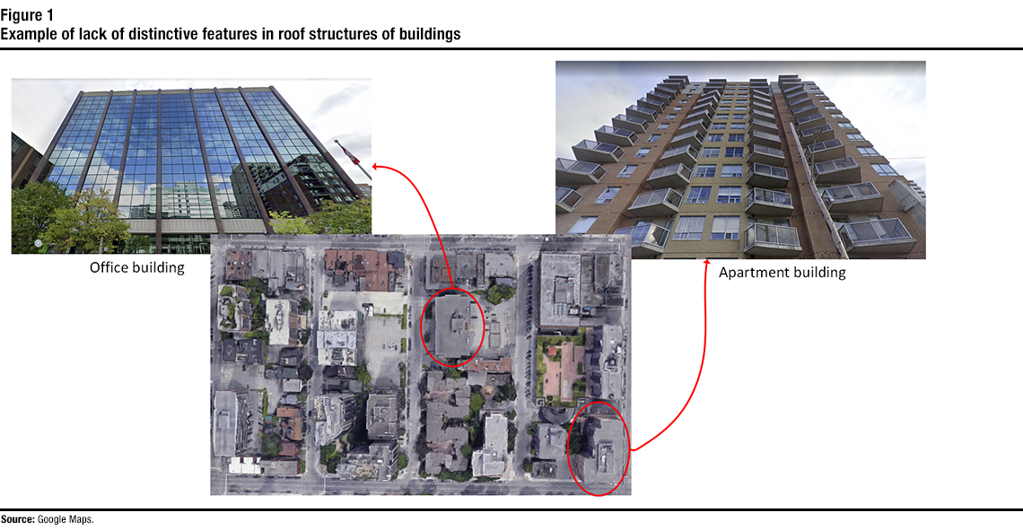
Description of figure 1
This is a figure that shows street-view images of an office building and an apartment building, and an aerial image that shows the top of both buildings. The figure illustrates how street-view images can show distinctive features in buildings’ facades that might not be available in roof structures.Much work has been done in both academia and the industry to extract similar information on urban areas using remote sensing. For example, aerial or satellite imagery has been used to collect information such as urban land use and land cover (Giri, 2016). While aerial and satellite imagery can be used to extract such information at the area or block level, it remains challenging to use such data to classify the type of individual buildings. This is because such images do not provide a view of the building façades, where the distinctions between different types of buildings are usually apparent. There are no explicit distinctions between the roofs of different types of buildings, as shown in Figure 1 (e.g., apartment building vs. office building), making it difficult to use such imagery for extracting building type.
Street-view imagery provides a close view of building façades, and hence can be used to extract a building type. There has been some effort in the literature to extract data from street-view images. This includes various applications such as estimating urban land use (Li et al., 2017) and the demographic makeup of neighbourhoods (Gebru et al., 2017). Moreover, street-view imagery has been used for building instance classification (Kang et al., 2018). Results from the work above show that street-view images can indeed provide a rich source of information in multiple applications.
In this paper, convolutional neural networks (CNNs) are finetuned to classify buildings into different types (e.g., house, apartment, industrial) using their street-view images. The datasets used for finetuning and testing the CNNs were collected by (Kang et al., 2018) and made publicly available for use. Features of the façade structures of the buildings that appear in street-view images can be captured by CNNs and used for classification purposes. The training set was manually investigated and cleaned to reduce errors introduced by automatic labelling. Thereafter, multiple state-of-the-art CNNs were finetuned to accomplish the classification task with the improved dataset. The training and validation performance of each trained CNN was measured. Furthermore, the trained CNNs were evaluated on a separate test set of street-view imagery (also provided by the benchmarking set) taken from cities different from the ones in the training set. Obtained results show that cleaning of the dataset and hyperparameter tuning achieved considerable improvements over the results by (Kang et al., 2018).
The rest of this paper is structured as follows: Section 2 provides a quick overview of deep learning and its use in computer vision, Section 3 discusses the datasets and the training of the CNNs used in this analysis, Section 4 presents the obtained results, and Section 5 concludes this paper.
2 Deep learning and convolutional neural networks
The continuous advancement of processing resources (e.g., GPUs, cloud resources) and the increasing availability of publicly available and large datasets for analysis and model development have increased the popularity of machine learning and deep learning to capture intricate structures of large-scale data (Voulodimos et al., 2018). Deep learning is currently a very popular field that has applications in many areas such as computer and machine vision, speech recognition, and natural language processing.
Computer vision is a field where deep learning has been increasingly deployed to extract information from different types of imagery. This increasing popularity of deep learning-based approaches is because they usually provide better results in computer vision than traditional methods where features are explicitly engineered (Voulodimos et al., 2018). A particular class of neural networks, CNNs, is increasingly popular in computer vision and used for various tasks such as object detection and classification, semantic segmentation, motion tracking, and face recognition. This is due to the efficiency of CNNs for such tasks, as they can reduce the number of parameters without losing the quality of the resulting models (Voulodimos et al., 2018). This is important because of the high dimensionality of images. Dimensionality refers to the number of features (variables) used as the input of the prediction or classification model. When images are used as the input of a model, the number of features is usually the number of colour values of the pixels in the image. For instance, for a 512×512 Red Green Blue image, the number of features would be the number of pixels multiplied by three (because of three colour channels), which is 786,432 in this case. This is a high number of features, and, hence, the use of efficient processing techniques in such a case is crucial.
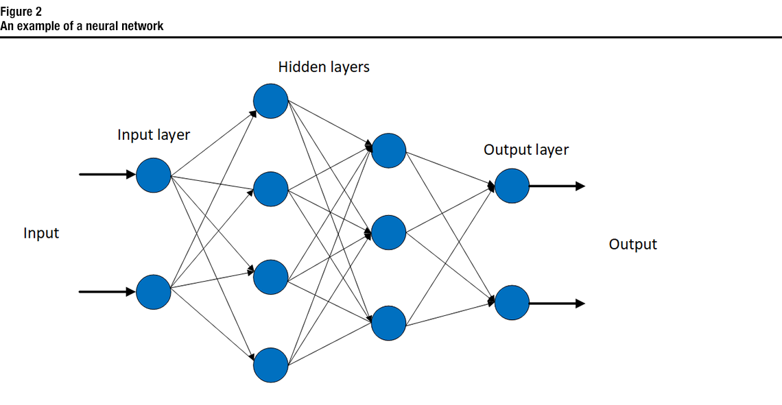
Description of figure 2
This is a figure that shows an example of a neural network composed of an input layer, two hidden layers, and an output layer.A neural network is composed of a group of connected nodes or units called artificial neurons (Dong et al., 2021). These neurons loosely model the neurons in a biological brain. An artificial neuron receives a signal, value or real number (or a collection of signals), then processes the input (applies some non-linear function), and may send it to other neurons connected to it. Figure 2 shows an example of a neural network. The neurons are usually structured into layers, where layers may perform different transformations on their inputs. Signals are received at the input layer, and travel through one or multiple hidden layers into the output layer. A deep neural network is a neural network with multiple hidden layers. Fully connected layers are common in deep neural networks. As their name implies, the neurons in a fully connected layer have full connections to the outputs from the previous layer (see Figure 2). The outputs of a fully connected layer can be used as the classification result or fed into another layer.
A CNN is a type of deep neural network that is usually composed of three types of layers: convolutional layers, pooling layers and fully connected layers (Voulodimos et al., 2018). A fully connected layer is usually preceded by the first two types, which take the input data (usually an image) and transform them into a feature vector. Pooling layers are usually used between convolutional layers. They perform subsampling on the input of a convolutional layer to reduce its dimensionality. This reduction in the spatial dimension serves two purposes: it reduces the computational complexity and also reduces overfitting.Note Fully connected layers are commonly used after the convolutional and pooling layers to transform the two-dimensional feature maps to a one-dimensional feature vector.
3 Training of convolutional neural networks for building type classification
3.1 Dataset used
Easily accessible street-view imagery is spreading rapidly. Over the past few years, several platforms for street-view imagery have emerged, which offer different terms and conditions of services and different degrees of “openness.” Google Street View (Google, 2020), Mapillary (Mapillary, 2014) and OpenStreetCam (Grab Holdings, 2009) are examples of such platforms. Street-view imagery provides remarkable opportunities to enrich existing data on buildings with complementary information relevant for further economic and spatial analyses. Furthermore, such imagery can be used on a large scale as it generally provides good geographic coverage and is easily accessible.
In a previous analysis conducted by the author of this paper, the Google Street View Static Application Programming Interface (API) was used to source test images for another computer vision project (Al-Habashna, 2020, 2021) because this API provides extensive coverage (especially in urban areas) worldwide. The Google Street View Static API allows downloading static (non-interactive) street-view panorama or thumbnail with Hypertext Transfer Protocol (HTTP) requests (Google, 2020). A standard HTTP request can be used to request the street-view image, and a static image is returned. Several parameters can be provided with the request, such as the camera pitch (i.e., angle of the camera relative to the Street View vehicle) and the angle of view (i.e., the angular extent of the scene that is imaged by a camera).
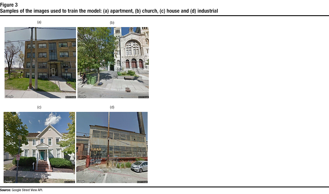
Description of figure 3
This figure shows samples of the images used to train the models, i.e., street view images of (a) apartment (b) church (c) house (d) and industrial buildings.The present analysis makes use of a large set of street-view images generated from the Google Street View Static API and made publicly available by (Kang et al., 2018). The dataset was collected and structured to be used to build models for building instance classification. The used benchmark dataset contains 19,658 images. These images are from different cities in Canada and the United States (e.g., Montréal, New York). The images are divided into the following eight different classes: apartment, church, garage, house, industrial, office building, retail and roof. The labels of these images were obtained from OpenStreetMap (OSM) (OpenStreetMap, 2004). OSM provides certain tags that are associated with addresses (e.g., house, single house, apartment). These tags were used to infer the correct label of the image. For example, an image of an address with the single-house tag is labelled as a house. Each class contains about 2,500 images. The images have a spatial resolution of 512×512 pixels, taken with a pitch value of 10 and the default angle-of-view value (90 degrees). Samples of the used images are shown in Figure 3.
Because of the automatic approach of labelling used to prepare the dataset (based on OSM tags), there are many errors in the labelling of the training set (e.g., a house might be labelled as an apartment or a garage). As a result, the dataset labelling was manually investigated and corrected. In Section 4, we further discuss the errors in training set labelling and show how correction of image labelling can achieve considerable performance improvement on the models’ classification accuracy.
3.2 Trained convolutional neural networks
Since training a CNN usually involves millions of parameters and requires a very large dataset, finetuning is a common practice when training a CNN. With finetuning, a target model is created from a source model. The target model is the model that needs to be trained, while the source model is a model that is already trained for a different but relevant problem. The source model is used as the starting point, instead of training the target model from scratch. An example of this is using a model for classifying animals (e.g., cat, dog, bear) as the source model and finetuning it to build a model that classifies images of dogs into different breeds (e.g., golden retriever, Labrador retriever).
The target model usually replicates all model designs and their parameters (e.g., number and size of the hidden layers and their parameters) of the source model, except the output layer (Quinn, 2019). This is particularly useful when the copied parameters that contain the knowledge learned from the source dataset are applicable to the target dataset. As the size of the output layer (number of neurons) of a classification model is usually equal to the number of classes, an output layer whose output size is the number of target dataset categories is used in the target model to account for the difference in the number of classes between the source and target models. Thereafter, the parameters of the output layer are randomly initialized, and the target model is then finetuned with the target dataset.
There are many CNNs that have been trained on large datasets and can be used for finetuning. Examples of such CNNs are those trained on the ImageNet dataset (Russakovsky et al., 2015), which can be finetuned with smaller datasets and used for other purposes. In this analysis, multiple state-of-the-art CNN architectures have been finetuned with the building dataset discussed above. This is done by finetuning all the convolutional layers of these CNNs as they were presented by (Kang et al., 2018). This includes multiple variations of the ResNet architecture (He et al., 2016) as well as the VGG16 architecture (Simonyan et al., 2015).
In this paper, two different models were trained with the architectures above. Multiple versions of the second model were also trained to compare the effect of hyperparameter tuning and labelling correction. Below, the developed models are listed and described:
- Binary model: a binary model that classifies buildings into one of two classes. These classes are residential and non-residential.
- Multi-class model: a model that classifies a building into eight different classes. These classes are apartment, church, garage, house, industrial, office building, retail and roof. Below, the different versions of this model are listed:
- Version 1: A model trained with the same parameters as in (Kang et al., 2018) except for dropout.
- Version 2: A model trained with different parameters and provided some improvement.
- Version 3: A model with the same parameters as Version 2, but with a dataset that was manually updated to correct labelling.
4 Results
4.1 Binary-classification model
In this section, the results of the binary model are discussed. This model classifies a building into two types: residential and non-residential. For this purpose, the set of images was structured into two types. The first type is residential, which contained houses and apartment buildings. The second type is non-residential, which contained the other classes (office buildings, industrial buildings, etc.). Then, the dataset was used to finetune the CNN architectures (i.e., ResNet18, ResNet34 and VGG16). As previously mentioned, each class in the image set contains about 2,500 images. The image set was split into training and validation sets, comprising 80% and 20% of the whole set, respectively. The fully connected layers of these architectures were randomly initialized, while the original values of the parameters of the convolutional layers were used. The same parameters used by (Kang et al., 2018) were adopted for this model. The stochastic gradient descent algorithm was used with a learning rate of , a momentum value of p = 0.9, and a decay factor (on the learning rate) of 0.1 per 30 epochs. Furthermore, cross-entropy loss was used in the training phase with a weight decay of 10-5. The input images were downsized to 256×256 pixels. Afterwards, data augmentation was also used by randomly cropping the input images into 224×224 pixels and randomly applying horizontal flipping on the cropped images before feeding them into a network. The CNNs were implemented with PyTorch (PyTorch, 2016) and were trained on a notebook server with NVIDIA V100 32GB-GPU.
Figure 4 shows the learning curve for the training and validation phases of the trained CNNs until 80 epochs. From the learning curves, one can see that all the CNNs converge by epoch 40. This means that no further improvement (or considerable change) is achieved on the accuracies for all the trained networks after epoch 40. The best achieved training and validation accuracies for the three architectures are listed in Table 1. From the training accuracy curves and the results in the table, one can see that the best training accuracy was achieved with ResNet34, where a training accuracy of 0.95 was achieved. However, the other CNNs achieved close values of training accuracy.
Validation accuracy is the accuracy achieved with the validation dataset (a dataset that the model has not seen in the training phase). VGG16 achieved the best validation accuracy (0.90). The other CNNs achieved close values for the validation accuracy.
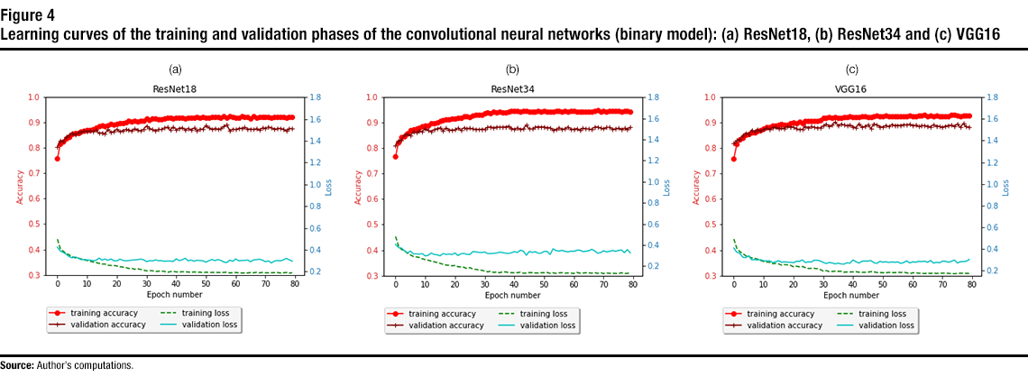
Description of figure 4
This figure contains three subfigures, each for a different architecture (e.g., ResNet18). Each subfigure shows the accuracy and loss versus the epoch number (for the training and validation phases) for the trained binary models. | Epoch number | ResNet18 | ResNet34 | VGG16 | |||||||||
|---|---|---|---|---|---|---|---|---|---|---|---|---|
| training accuracy | validation accuracy | training loss | validation loss | training accuracy | validation accuracy | training loss | validation loss | training accuracy | validation accuracy | training loss | validation loss | |
| 1 | 0.758 | 0.803 | 0.497 | 0.424 | 0.767 | 0.810 | 0.481 | 0.407 | 0.760 | 0.818 | 0.491 | 0.408 |
| 2 | 0.817 | 0.829 | 0.409 | 0.389 | 0.823 | 0.829 | 0.392 | 0.375 | 0.815 | 0.830 | 0.406 | 0.369 |
| 3 | 0.825 | 0.827 | 0.385 | 0.375 | 0.843 | 0.832 | 0.358 | 0.370 | 0.834 | 0.835 | 0.375 | 0.360 |
| 4 | 0.838 | 0.842 | 0.366 | 0.358 | 0.846 | 0.852 | 0.344 | 0.347 | 0.839 | 0.850 | 0.357 | 0.324 |
| 5 | 0.844 | 0.852 | 0.353 | 0.337 | 0.860 | 0.854 | 0.323 | 0.326 | 0.853 | 0.859 | 0.337 | 0.320 |
| 6 | 0.854 | 0.859 | 0.338 | 0.327 | 0.869 | 0.849 | 0.306 | 0.342 | 0.855 | 0.855 | 0.329 | 0.337 |
| 7 | 0.858 | 0.851 | 0.326 | 0.335 | 0.875 | 0.863 | 0.292 | 0.315 | 0.861 | 0.871 | 0.318 | 0.299 |
| 8 | 0.858 | 0.861 | 0.323 | 0.323 | 0.876 | 0.860 | 0.288 | 0.316 | 0.862 | 0.866 | 0.313 | 0.302 |
| 9 | 0.865 | 0.861 | 0.315 | 0.310 | 0.880 | 0.867 | 0.283 | 0.314 | 0.867 | 0.874 | 0.306 | 0.299 |
| 10 | 0.867 | 0.869 | 0.308 | 0.311 | 0.886 | 0.866 | 0.269 | 0.318 | 0.872 | 0.866 | 0.294 | 0.300 |
| 11 | 0.869 | 0.864 | 0.302 | 0.306 | 0.887 | 0.875 | 0.262 | 0.297 | 0.877 | 0.874 | 0.285 | 0.291 |
| 12 | 0.871 | 0.868 | 0.295 | 0.305 | 0.888 | 0.870 | 0.256 | 0.303 | 0.882 | 0.879 | 0.279 | 0.290 |
| 13 | 0.874 | 0.863 | 0.288 | 0.301 | 0.897 | 0.866 | 0.248 | 0.325 | 0.882 | 0.874 | 0.277 | 0.291 |
| 14 | 0.879 | 0.870 | 0.282 | 0.303 | 0.899 | 0.873 | 0.241 | 0.311 | 0.888 | 0.881 | 0.263 | 0.275 |
| 15 | 0.885 | 0.858 | 0.276 | 0.323 | 0.900 | 0.877 | 0.235 | 0.307 | 0.888 | 0.883 | 0.266 | 0.282 |
| 16 | 0.889 | 0.859 | 0.269 | 0.306 | 0.905 | 0.880 | 0.226 | 0.298 | 0.892 | 0.876 | 0.262 | 0.291 |
| 17 | 0.887 | 0.856 | 0.269 | 0.315 | 0.909 | 0.869 | 0.218 | 0.319 | 0.894 | 0.878 | 0.251 | 0.277 |
| 18 | 0.887 | 0.872 | 0.258 | 0.303 | 0.913 | 0.879 | 0.210 | 0.311 | 0.891 | 0.878 | 0.255 | 0.281 |
| 19 | 0.894 | 0.862 | 0.256 | 0.316 | 0.913 | 0.871 | 0.208 | 0.315 | 0.890 | 0.884 | 0.253 | 0.277 |
| 20 | 0.891 | 0.865 | 0.256 | 0.299 | 0.915 | 0.871 | 0.203 | 0.310 | 0.896 | 0.883 | 0.249 | 0.277 |
| 21 | 0.894 | 0.874 | 0.251 | 0.298 | 0.915 | 0.872 | 0.207 | 0.325 | 0.899 | 0.883 | 0.236 | 0.273 |
| 22 | 0.898 | 0.863 | 0.244 | 0.314 | 0.919 | 0.879 | 0.195 | 0.301 | 0.897 | 0.876 | 0.241 | 0.286 |
| 23 | 0.899 | 0.869 | 0.242 | 0.304 | 0.919 | 0.871 | 0.192 | 0.317 | 0.903 | 0.873 | 0.235 | 0.285 |
| 24 | 0.902 | 0.873 | 0.237 | 0.297 | 0.923 | 0.880 | 0.190 | 0.320 | 0.898 | 0.874 | 0.238 | 0.298 |
| 25 | 0.906 | 0.872 | 0.229 | 0.301 | 0.925 | 0.878 | 0.177 | 0.313 | 0.907 | 0.884 | 0.228 | 0.275 |
| 26 | 0.905 | 0.866 | 0.230 | 0.305 | 0.921 | 0.878 | 0.186 | 0.310 | 0.907 | 0.880 | 0.220 | 0.281 |
| 27 | 0.906 | 0.875 | 0.221 | 0.307 | 0.927 | 0.875 | 0.174 | 0.338 | 0.908 | 0.885 | 0.221 | 0.279 |
| 28 | 0.905 | 0.871 | 0.226 | 0.310 | 0.932 | 0.874 | 0.169 | 0.335 | 0.907 | 0.881 | 0.221 | 0.296 |
| 29 | 0.908 | 0.867 | 0.220 | 0.314 | 0.931 | 0.873 | 0.165 | 0.331 | 0.906 | 0.880 | 0.218 | 0.296 |
| 30 | 0.908 | 0.874 | 0.213 | 0.309 | 0.932 | 0.875 | 0.161 | 0.329 | 0.911 | 0.879 | 0.210 | 0.289 |
| 31 | 0.915 | 0.887 | 0.206 | 0.291 | 0.938 | 0.874 | 0.153 | 0.334 | 0.919 | 0.887 | 0.196 | 0.276 |
| 32 | 0.911 | 0.878 | 0.209 | 0.300 | 0.939 | 0.882 | 0.147 | 0.320 | 0.918 | 0.895 | 0.199 | 0.266 |
| 33 | 0.915 | 0.872 | 0.207 | 0.298 | 0.936 | 0.883 | 0.151 | 0.318 | 0.922 | 0.886 | 0.191 | 0.275 |
| 34 | 0.916 | 0.868 | 0.201 | 0.307 | 0.943 | 0.880 | 0.140 | 0.322 | 0.918 | 0.890 | 0.192 | 0.271 |
| 35 | 0.914 | 0.873 | 0.203 | 0.300 | 0.941 | 0.883 | 0.144 | 0.324 | 0.921 | 0.903 | 0.195 | 0.262 |
| 36 | 0.914 | 0.872 | 0.205 | 0.300 | 0.944 | 0.882 | 0.138 | 0.332 | 0.920 | 0.888 | 0.193 | 0.268 |
| 37 | 0.917 | 0.879 | 0.201 | 0.295 | 0.940 | 0.882 | 0.145 | 0.328 | 0.918 | 0.895 | 0.194 | 0.262 |
| 38 | 0.919 | 0.882 | 0.193 | 0.297 | 0.940 | 0.883 | 0.145 | 0.323 | 0.923 | 0.891 | 0.186 | 0.261 |
| 39 | 0.918 | 0.871 | 0.199 | 0.296 | 0.943 | 0.887 | 0.140 | 0.320 | 0.922 | 0.889 | 0.187 | 0.272 |
| 40 | 0.916 | 0.883 | 0.201 | 0.294 | 0.945 | 0.878 | 0.138 | 0.327 | 0.923 | 0.891 | 0.187 | 0.269 |
| 41 | 0.919 | 0.871 | 0.197 | 0.317 | 0.945 | 0.874 | 0.138 | 0.338 | 0.923 | 0.884 | 0.188 | 0.298 |
| 42 | 0.917 | 0.878 | 0.196 | 0.301 | 0.946 | 0.879 | 0.138 | 0.330 | 0.923 | 0.881 | 0.190 | 0.281 |
| 43 | 0.920 | 0.880 | 0.198 | 0.309 | 0.942 | 0.875 | 0.142 | 0.351 | 0.923 | 0.896 | 0.185 | 0.270 |
| 44 | 0.916 | 0.871 | 0.198 | 0.322 | 0.945 | 0.876 | 0.133 | 0.342 | 0.923 | 0.882 | 0.184 | 0.286 |
| 45 | 0.919 | 0.876 | 0.196 | 0.300 | 0.945 | 0.890 | 0.135 | 0.303 | 0.925 | 0.886 | 0.184 | 0.288 |
| 46 | 0.919 | 0.871 | 0.193 | 0.306 | 0.942 | 0.876 | 0.139 | 0.339 | 0.922 | 0.892 | 0.186 | 0.288 |
| 47 | 0.920 | 0.878 | 0.197 | 0.295 | 0.944 | 0.875 | 0.139 | 0.331 | 0.922 | 0.878 | 0.190 | 0.292 |
| 48 | 0.920 | 0.869 | 0.194 | 0.304 | 0.944 | 0.883 | 0.135 | 0.337 | 0.924 | 0.895 | 0.188 | 0.273 |
| 49 | 0.920 | 0.874 | 0.194 | 0.302 | 0.946 | 0.883 | 0.135 | 0.323 | 0.927 | 0.892 | 0.182 | 0.267 |
| 50 | 0.923 | 0.874 | 0.190 | 0.298 | 0.944 | 0.883 | 0.138 | 0.324 | 0.923 | 0.884 | 0.182 | 0.285 |
| 51 | 0.920 | 0.888 | 0.194 | 0.286 | 0.945 | 0.883 | 0.138 | 0.340 | 0.924 | 0.883 | 0.181 | 0.278 |
| 52 | 0.918 | 0.879 | 0.193 | 0.300 | 0.942 | 0.880 | 0.140 | 0.339 | 0.927 | 0.890 | 0.180 | 0.281 |
| 53 | 0.922 | 0.873 | 0.192 | 0.311 | 0.944 | 0.880 | 0.132 | 0.311 | 0.924 | 0.885 | 0.184 | 0.276 |
| 54 | 0.921 | 0.876 | 0.193 | 0.301 | 0.944 | 0.871 | 0.136 | 0.364 | 0.924 | 0.893 | 0.182 | 0.280 |
| 55 | 0.922 | 0.875 | 0.191 | 0.310 | 0.945 | 0.874 | 0.132 | 0.347 | 0.925 | 0.890 | 0.181 | 0.277 |
| 56 | 0.918 | 0.875 | 0.191 | 0.303 | 0.945 | 0.880 | 0.136 | 0.343 | 0.924 | 0.890 | 0.185 | 0.280 |
| 57 | 0.924 | 0.885 | 0.192 | 0.288 | 0.943 | 0.875 | 0.138 | 0.349 | 0.925 | 0.890 | 0.182 | 0.267 |
| 58 | 0.917 | 0.891 | 0.194 | 0.283 | 0.947 | 0.876 | 0.134 | 0.340 | 0.924 | 0.893 | 0.186 | 0.274 |
| 59 | 0.924 | 0.868 | 0.188 | 0.305 | 0.943 | 0.884 | 0.135 | 0.336 | 0.926 | 0.891 | 0.180 | 0.290 |
| 60 | 0.921 | 0.874 | 0.190 | 0.294 | 0.946 | 0.874 | 0.135 | 0.342 | 0.927 | 0.894 | 0.172 | 0.271 |
| 61 | 0.919 | 0.872 | 0.191 | 0.316 | 0.947 | 0.874 | 0.131 | 0.341 | 0.925 | 0.888 | 0.179 | 0.281 |
| 62 | 0.919 | 0.877 | 0.188 | 0.299 | 0.943 | 0.877 | 0.141 | 0.350 | 0.925 | 0.890 | 0.180 | 0.278 |
| 63 | 0.926 | 0.878 | 0.186 | 0.302 | 0.943 | 0.870 | 0.134 | 0.352 | 0.927 | 0.884 | 0.176 | 0.285 |
| 64 | 0.923 | 0.881 | 0.188 | 0.303 | 0.942 | 0.879 | 0.135 | 0.338 | 0.929 | 0.888 | 0.176 | 0.284 |
| 65 | 0.923 | 0.874 | 0.187 | 0.306 | 0.944 | 0.876 | 0.137 | 0.341 | 0.929 | 0.888 | 0.172 | 0.287 |
| 66 | 0.917 | 0.874 | 0.191 | 0.291 | 0.944 | 0.875 | 0.136 | 0.346 | 0.926 | 0.886 | 0.178 | 0.277 |
| 67 | 0.924 | 0.873 | 0.189 | 0.307 | 0.944 | 0.874 | 0.134 | 0.359 | 0.929 | 0.884 | 0.174 | 0.294 |
| 68 | 0.919 | 0.876 | 0.193 | 0.310 | 0.945 | 0.883 | 0.138 | 0.345 | 0.924 | 0.892 | 0.179 | 0.269 |
| 69 | 0.923 | 0.870 | 0.188 | 0.314 | 0.948 | 0.883 | 0.132 | 0.322 | 0.927 | 0.887 | 0.173 | 0.277 |
| 70 | 0.921 | 0.879 | 0.192 | 0.305 | 0.943 | 0.879 | 0.138 | 0.329 | 0.924 | 0.886 | 0.177 | 0.272 |
| 71 | 0.921 | 0.878 | 0.189 | 0.290 | 0.946 | 0.876 | 0.129 | 0.345 | 0.926 | 0.882 | 0.176 | 0.287 |
| 72 | 0.922 | 0.883 | 0.188 | 0.298 | 0.943 | 0.881 | 0.135 | 0.335 | 0.925 | 0.887 | 0.178 | 0.286 |
| 73 | 0.920 | 0.879 | 0.189 | 0.280 | 0.945 | 0.882 | 0.132 | 0.341 | 0.926 | 0.888 | 0.175 | 0.278 |
| 74 | 0.921 | 0.874 | 0.190 | 0.296 | 0.947 | 0.875 | 0.134 | 0.348 | 0.930 | 0.891 | 0.172 | 0.285 |
| 75 | 0.921 | 0.876 | 0.192 | 0.302 | 0.946 | 0.876 | 0.131 | 0.341 | 0.930 | 0.886 | 0.171 | 0.298 |
| 76 | 0.922 | 0.877 | 0.187 | 0.298 | 0.947 | 0.879 | 0.130 | 0.349 | 0.929 | 0.895 | 0.173 | 0.270 |
| 77 | 0.922 | 0.875 | 0.188 | 0.307 | 0.944 | 0.874 | 0.137 | 0.354 | 0.926 | 0.882 | 0.176 | 0.282 |
| 78 | 0.919 | 0.866 | 0.192 | 0.321 | 0.947 | 0.878 | 0.129 | 0.328 | 0.927 | 0.896 | 0.176 | 0.283 |
| 79 | 0.923 | 0.876 | 0.186 | 0.308 | 0.946 | 0.874 | 0.132 | 0.357 | 0.927 | 0.884 | 0.175 | 0.286 |
| 80 | 0.923 | 0.875 | 0.189 | 0.296 | 0.944 | 0.882 | 0.137 | 0.326 | 0.928 | 0.881 | 0.174 | 0.303 |
| Architecture | Training accuracy | Validation accuracy |
|---|---|---|
| ResNet18 | 0.93 | 0.89 |
| ResNet34 | 0.95 | 0.89 |
| VGG16 | 0.93 | 0.90 |
None of the finetuned CNNs show a significant overfitting behaviour, with the VGG16 having the smallest difference between the training and validation accuracies. Overfitting is an undesirable result in model training, where the model represents the training data too well, as opposed to being generic and providing high prediction or classification accuracy for any dataset. ResNet34 has the highest difference between the training and validation accuracy, because of the high number of parameters in this network.
4.2 Multi-class model
As previously mentioned, a second model is built with four CNN architectures to classify buildings into eight types: apartment, church, garage, house, industrial, office building, retail and roof. Three versions of each CNN architecture were trained. The three versions of the multi-class model are listed again here for clarity:
- Version 1: A model trained with the same parameters as in (Kang et al., 2018) except for dropout.
- Version 2: A model trained with different parameters and provided some improvement.
- Version 3: A model with the same parameters as Version 2, but with a dataset that was manually updated to correct labelling.
Version 1
Figure 5 shows the learning curve for the training and validation phases for the trained CNNs (i.e., ResNet18, ResNet34, ResNet50 and VGG16) until 80 epochs. From the learning curves, one can see that all the CNNs converge by epoch 60, i.e., no further improvement is achieved on the accuracies for all the trained networks after epoch 60. The best achieved training and validation accuracies for all the trained CNNs are also listed in Table 2. From the training accuracy curves and the results in the table, one can see that the best training accuracy was achieved with ResNet50, where a training accuracy of 0.92 was achieved. Other CNNs achieved training accuracies around 0.80. Validation accuracy is the accuracy achieved with the validation dataset (a dataset that the model has not seen in the training phase). The best validation accuracy (0.70) was achieved with VGG16 and ResNet50, while other CNNs obtained close validation accuracy (0.67 for ResNet and 0.69 for ResNet34). The results show that some overfitting can be seen with ResNet34 and ResNet50. As explained above, overfitting is an undesirable result in model training where the model represents the training data too well, as opposed to being generic and providing high prediction or classification accuracy for any dataset. For ResNet34 and ResNet50, overfitting can be seen as the training accuracy being higher than the validation accuracy. This is a result of the large number of parameters in these networks.
Figure 6 shows samples of the output obtained on a test set. The test set comprises images collected from cities other than the cities in the training set. The results presented here are those obtained with the VGG16 network, as it provided the best validation accuracy and had the least overfitting behaviour. The test set comprises about 2,000 images (each class contains about 250 images). The classification accuracy achieved with VGG16 on this set was 0.59, which matches the results of (Kang et al., 2018). Figure 6 shows samples of the results obtained with the VGG16 architecture on the aforementioned test set. The samples show many examples of cases where the model classified the images correctly. However, there are cases where the images were misclassified. For instance, a garage may be misclassified as a house (or vice versa), as the garage is part of a house in most cases. At the top-right corner, we see a house building that was originally mislabelled as a roof. Inspection of the dataset (training and test sets) showed that there are many mislabelled images. As a result, a manual correction of the labelling of the data is done, and a new model (Version 3) is trained with the improved dataset.
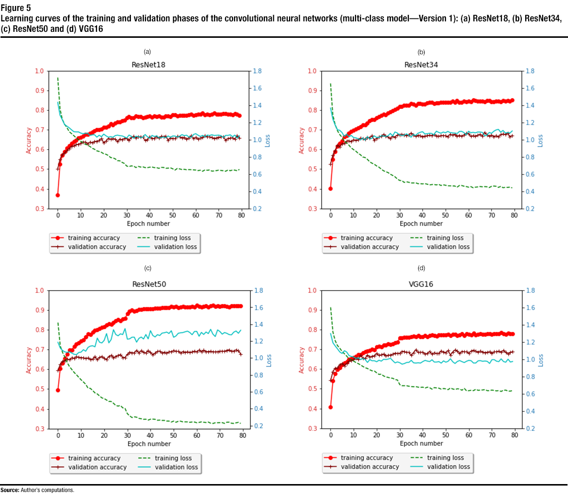
Description of figure 5
This figure contains four subfigures, each for a different architecture (e.g., ResNet18). Each subfigure shows the accuracy and loss versus the epoch number (for the training and validation phases) for the trained multi-class models (version 1). | Epoch number | ResNet18 | ResNet34 | ResNet50 | VGG16 | ||||||||||||
|---|---|---|---|---|---|---|---|---|---|---|---|---|---|---|---|---|
| training accuracy | validation accuracy | training loss | validation loss | training accuracy | validation accuracy | training loss | validation loss | training accuracy | validation accuracy | training loss | validation loss | training accuracy | validation accuracy | training loss | validation loss | |
| 1 | 0.369 | 0.501 | 1.723 | 1.435 | 0.401 | 0.526 | 1.655 | 1.369 | 0.496 | 0.594 | 1.419 | 1.186 | 0.379 | 0.517 | 1.695 | 1.376 |
| 2 | 0.526 | 0.550 | 1.356 | 1.284 | 0.550 | 0.571 | 1.287 | 1.239 | 0.605 | 0.625 | 1.142 | 1.117 | 0.510 | 0.560 | 1.375 | 1.254 |
| 3 | 0.569 | 0.574 | 1.235 | 1.232 | 0.589 | 0.595 | 1.178 | 1.170 | 0.631 | 0.641 | 1.065 | 1.089 | 0.552 | 0.579 | 1.272 | 1.193 |
| 4 | 0.590 | 0.583 | 1.178 | 1.174 | 0.615 | 0.623 | 1.105 | 1.116 | 0.655 | 0.645 | 1.011 | 1.072 | 0.578 | 0.597 | 1.209 | 1.144 |
| 5 | 0.606 | 0.594 | 1.140 | 1.157 | 0.632 | 0.613 | 1.059 | 1.108 | 0.675 | 0.652 | 0.946 | 1.067 | 0.597 | 0.610 | 1.165 | 1.133 |
| 6 | 0.620 | 0.605 | 1.093 | 1.138 | 0.645 | 0.629 | 1.027 | 1.083 | 0.697 | 0.648 | 0.897 | 1.073 | 0.614 | 0.622 | 1.122 | 1.087 |
| 7 | 0.631 | 0.616 | 1.070 | 1.114 | 0.664 | 0.630 | 0.981 | 1.038 | 0.699 | 0.658 | 0.864 | 1.058 | 0.613 | 0.631 | 1.097 | 1.078 |
| 8 | 0.639 | 0.618 | 1.047 | 1.093 | 0.669 | 0.642 | 0.963 | 1.065 | 0.716 | 0.657 | 0.829 | 1.043 | 0.633 | 0.637 | 1.070 | 1.069 |
| 9 | 0.647 | 0.625 | 1.021 | 1.091 | 0.682 | 0.644 | 0.935 | 1.034 | 0.727 | 0.664 | 0.801 | 1.040 | 0.633 | 0.633 | 1.059 | 1.048 |
| 10 | 0.658 | 0.627 | 0.999 | 1.091 | 0.692 | 0.641 | 0.904 | 1.049 | 0.733 | 0.661 | 0.771 | 1.065 | 0.646 | 0.639 | 1.021 | 1.053 |
| 11 | 0.661 | 0.633 | 0.981 | 1.076 | 0.699 | 0.649 | 0.884 | 1.025 | 0.742 | 0.659 | 0.742 | 1.070 | 0.651 | 0.641 | 1.007 | 1.024 |
| 12 | 0.668 | 0.638 | 0.965 | 1.069 | 0.703 | 0.647 | 0.866 | 1.021 | 0.751 | 0.658 | 0.716 | 1.099 | 0.661 | 0.647 | 0.989 | 1.026 |
| 13 | 0.678 | 0.637 | 0.946 | 1.073 | 0.710 | 0.650 | 0.841 | 1.010 | 0.765 | 0.656 | 0.689 | 1.080 | 0.669 | 0.648 | 0.962 | 1.021 |
| 14 | 0.677 | 0.629 | 0.938 | 1.074 | 0.716 | 0.658 | 0.824 | 0.996 | 0.779 | 0.658 | 0.643 | 1.126 | 0.674 | 0.657 | 0.947 | 1.017 |
| 15 | 0.681 | 0.637 | 0.921 | 1.049 | 0.725 | 0.654 | 0.798 | 1.020 | 0.776 | 0.651 | 0.640 | 1.141 | 0.677 | 0.655 | 0.940 | 1.021 |
| 16 | 0.688 | 0.635 | 0.899 | 1.056 | 0.725 | 0.653 | 0.792 | 0.993 | 0.788 | 0.652 | 0.615 | 1.145 | 0.679 | 0.650 | 0.925 | 1.019 |
| 17 | 0.695 | 0.641 | 0.889 | 1.058 | 0.736 | 0.663 | 0.771 | 1.035 | 0.798 | 0.664 | 0.587 | 1.132 | 0.691 | 0.661 | 0.906 | 0.998 |
| 18 | 0.702 | 0.642 | 0.869 | 1.029 | 0.747 | 0.660 | 0.743 | 1.008 | 0.800 | 0.649 | 0.575 | 1.236 | 0.690 | 0.659 | 0.900 | 0.982 |
| 19 | 0.702 | 0.646 | 0.863 | 1.052 | 0.752 | 0.670 | 0.726 | 1.016 | 0.807 | 0.661 | 0.549 | 1.186 | 0.703 | 0.665 | 0.874 | 0.985 |
| 20 | 0.705 | 0.656 | 0.853 | 1.034 | 0.753 | 0.648 | 0.714 | 1.045 | 0.812 | 0.665 | 0.527 | 1.179 | 0.701 | 0.662 | 0.867 | 0.975 |
| 21 | 0.714 | 0.633 | 0.836 | 1.065 | 0.762 | 0.656 | 0.695 | 1.025 | 0.816 | 0.657 | 0.519 | 1.209 | 0.709 | 0.672 | 0.844 | 0.998 |
| 22 | 0.713 | 0.643 | 0.829 | 1.044 | 0.766 | 0.663 | 0.680 | 1.026 | 0.825 | 0.650 | 0.503 | 1.289 | 0.708 | 0.660 | 0.838 | 0.986 |
| 23 | 0.720 | 0.657 | 0.816 | 1.029 | 0.773 | 0.667 | 0.659 | 1.045 | 0.830 | 0.665 | 0.486 | 1.179 | 0.714 | 0.666 | 0.829 | 0.979 |
| 24 | 0.731 | 0.652 | 0.791 | 1.035 | 0.779 | 0.677 | 0.638 | 1.043 | 0.829 | 0.671 | 0.485 | 1.219 | 0.719 | 0.667 | 0.814 | 0.997 |
| 25 | 0.727 | 0.655 | 0.788 | 1.028 | 0.778 | 0.667 | 0.627 | 1.039 | 0.838 | 0.659 | 0.464 | 1.335 | 0.717 | 0.676 | 0.812 | 0.969 |
| 26 | 0.733 | 0.654 | 0.777 | 1.047 | 0.786 | 0.663 | 0.617 | 1.044 | 0.847 | 0.666 | 0.437 | 1.278 | 0.727 | 0.674 | 0.790 | 0.973 |
| 27 | 0.740 | 0.639 | 0.755 | 1.052 | 0.791 | 0.655 | 0.598 | 1.073 | 0.852 | 0.671 | 0.431 | 1.263 | 0.731 | 0.667 | 0.783 | 0.974 |
| 28 | 0.741 | 0.653 | 0.754 | 1.046 | 0.798 | 0.668 | 0.584 | 1.042 | 0.845 | 0.675 | 0.437 | 1.286 | 0.734 | 0.669 | 0.778 | 1.003 |
| 29 | 0.747 | 0.650 | 0.735 | 1.043 | 0.804 | 0.662 | 0.568 | 1.089 | 0.856 | 0.660 | 0.410 | 1.278 | 0.736 | 0.673 | 0.763 | 0.973 |
| 30 | 0.750 | 0.657 | 0.723 | 1.033 | 0.809 | 0.673 | 0.543 | 1.078 | 0.859 | 0.660 | 0.404 | 1.348 | 0.739 | 0.678 | 0.748 | 0.988 |
| 31 | 0.762 | 0.655 | 0.692 | 1.019 | 0.818 | 0.675 | 0.525 | 1.057 | 0.881 | 0.676 | 0.340 | 1.223 | 0.751 | 0.674 | 0.717 | 0.989 |
| 32 | 0.767 | 0.647 | 0.688 | 1.054 | 0.819 | 0.677 | 0.523 | 1.050 | 0.893 | 0.687 | 0.315 | 1.227 | 0.751 | 0.686 | 0.714 | 0.968 |
| 33 | 0.762 | 0.661 | 0.694 | 1.037 | 0.825 | 0.674 | 0.502 | 1.050 | 0.900 | 0.684 | 0.295 | 1.246 | 0.744 | 0.678 | 0.727 | 0.983 |
| 34 | 0.762 | 0.667 | 0.692 | 1.017 | 0.825 | 0.672 | 0.509 | 1.068 | 0.895 | 0.684 | 0.303 | 1.247 | 0.750 | 0.684 | 0.718 | 0.970 |
| 35 | 0.769 | 0.659 | 0.675 | 1.040 | 0.826 | 0.674 | 0.504 | 1.052 | 0.898 | 0.696 | 0.299 | 1.187 | 0.750 | 0.673 | 0.711 | 0.991 |
| 36 | 0.766 | 0.666 | 0.689 | 1.035 | 0.835 | 0.684 | 0.496 | 1.029 | 0.904 | 0.684 | 0.285 | 1.232 | 0.755 | 0.673 | 0.708 | 0.995 |
| 37 | 0.767 | 0.664 | 0.681 | 1.023 | 0.830 | 0.674 | 0.496 | 1.060 | 0.905 | 0.694 | 0.281 | 1.248 | 0.748 | 0.682 | 0.721 | 0.974 |
| 38 | 0.762 | 0.663 | 0.683 | 1.029 | 0.825 | 0.669 | 0.498 | 1.048 | 0.907 | 0.687 | 0.274 | 1.225 | 0.758 | 0.679 | 0.702 | 0.984 |
| 39 | 0.766 | 0.646 | 0.675 | 1.060 | 0.835 | 0.672 | 0.488 | 1.075 | 0.906 | 0.683 | 0.275 | 1.278 | 0.755 | 0.685 | 0.704 | 0.957 |
| 40 | 0.768 | 0.651 | 0.674 | 1.033 | 0.834 | 0.669 | 0.487 | 1.086 | 0.907 | 0.695 | 0.265 | 1.226 | 0.760 | 0.682 | 0.701 | 0.959 |
| 41 | 0.770 | 0.665 | 0.679 | 1.018 | 0.832 | 0.666 | 0.485 | 1.093 | 0.906 | 0.685 | 0.275 | 1.323 | 0.753 | 0.679 | 0.701 | 0.980 |
| 42 | 0.766 | 0.656 | 0.681 | 1.049 | 0.831 | 0.668 | 0.488 | 1.067 | 0.906 | 0.674 | 0.276 | 1.267 | 0.758 | 0.681 | 0.702 | 0.986 |
| 43 | 0.769 | 0.657 | 0.674 | 1.037 | 0.837 | 0.671 | 0.482 | 1.069 | 0.908 | 0.682 | 0.274 | 1.250 | 0.761 | 0.683 | 0.690 | 0.986 |
| 44 | 0.769 | 0.666 | 0.674 | 1.044 | 0.839 | 0.672 | 0.473 | 1.074 | 0.909 | 0.691 | 0.263 | 1.276 | 0.758 | 0.666 | 0.702 | 1.005 |
| 45 | 0.771 | 0.657 | 0.666 | 1.023 | 0.840 | 0.671 | 0.477 | 1.072 | 0.909 | 0.692 | 0.265 | 1.266 | 0.758 | 0.684 | 0.696 | 0.987 |
| 46 | 0.765 | 0.668 | 0.677 | 1.024 | 0.835 | 0.677 | 0.478 | 1.055 | 0.912 | 0.683 | 0.261 | 1.295 | 0.760 | 0.683 | 0.691 | 0.967 |
| 47 | 0.766 | 0.665 | 0.677 | 1.032 | 0.838 | 0.669 | 0.473 | 1.099 | 0.913 | 0.687 | 0.261 | 1.299 | 0.758 | 0.672 | 0.691 | 0.992 |
| 48 | 0.770 | 0.668 | 0.667 | 1.022 | 0.838 | 0.667 | 0.480 | 1.085 | 0.913 | 0.682 | 0.253 | 1.306 | 0.759 | 0.674 | 0.692 | 0.998 |
| 49 | 0.770 | 0.647 | 0.668 | 1.043 | 0.841 | 0.671 | 0.466 | 1.075 | 0.912 | 0.689 | 0.253 | 1.290 | 0.761 | 0.681 | 0.685 | 0.982 |
| 50 | 0.768 | 0.659 | 0.672 | 1.027 | 0.840 | 0.671 | 0.474 | 1.088 | 0.918 | 0.689 | 0.241 | 1.323 | 0.762 | 0.676 | 0.678 | 0.990 |
| 51 | 0.778 | 0.656 | 0.661 | 1.043 | 0.841 | 0.670 | 0.469 | 1.081 | 0.916 | 0.695 | 0.253 | 1.245 | 0.763 | 0.684 | 0.682 | 0.966 |
| 52 | 0.777 | 0.655 | 0.646 | 1.042 | 0.842 | 0.665 | 0.463 | 1.096 | 0.918 | 0.691 | 0.239 | 1.260 | 0.764 | 0.678 | 0.685 | 0.983 |
| 53 | 0.771 | 0.667 | 0.665 | 1.030 | 0.839 | 0.678 | 0.462 | 1.082 | 0.914 | 0.691 | 0.250 | 1.293 | 0.762 | 0.672 | 0.691 | 0.993 |
| 54 | 0.773 | 0.666 | 0.659 | 1.040 | 0.845 | 0.673 | 0.461 | 1.079 | 0.916 | 0.683 | 0.252 | 1.298 | 0.763 | 0.680 | 0.687 | 0.980 |
| 55 | 0.775 | 0.659 | 0.652 | 1.059 | 0.841 | 0.678 | 0.461 | 1.077 | 0.918 | 0.690 | 0.243 | 1.301 | 0.766 | 0.677 | 0.672 | 0.999 |
| 56 | 0.775 | 0.661 | 0.655 | 1.047 | 0.849 | 0.668 | 0.446 | 1.071 | 0.916 | 0.687 | 0.244 | 1.310 | 0.762 | 0.678 | 0.678 | 0.974 |
| 57 | 0.774 | 0.652 | 0.650 | 1.052 | 0.840 | 0.672 | 0.466 | 1.095 | 0.916 | 0.689 | 0.243 | 1.318 | 0.765 | 0.680 | 0.673 | 0.980 |
| 58 | 0.776 | 0.660 | 0.651 | 1.032 | 0.840 | 0.668 | 0.466 | 1.097 | 0.916 | 0.686 | 0.238 | 1.302 | 0.764 | 0.675 | 0.675 | 0.997 |
| 59 | 0.781 | 0.670 | 0.650 | 1.027 | 0.845 | 0.674 | 0.458 | 1.083 | 0.918 | 0.688 | 0.242 | 1.276 | 0.767 | 0.679 | 0.675 | 0.993 |
| 60 | 0.775 | 0.657 | 0.648 | 1.060 | 0.844 | 0.682 | 0.454 | 1.056 | 0.917 | 0.692 | 0.242 | 1.314 | 0.770 | 0.673 | 0.668 | 1.007 |
| 61 | 0.777 | 0.661 | 0.646 | 1.070 | 0.848 | 0.679 | 0.447 | 1.098 | 0.923 | 0.689 | 0.234 | 1.315 | 0.766 | 0.677 | 0.671 | 0.993 |
| 62 | 0.780 | 0.654 | 0.640 | 1.052 | 0.844 | 0.667 | 0.453 | 1.081 | 0.919 | 0.698 | 0.237 | 1.257 | 0.766 | 0.678 | 0.676 | 0.991 |
| 63 | 0.780 | 0.659 | 0.644 | 1.037 | 0.852 | 0.670 | 0.440 | 1.086 | 0.917 | 0.689 | 0.244 | 1.303 | 0.763 | 0.683 | 0.679 | 1.005 |
| 64 | 0.785 | 0.662 | 0.632 | 1.050 | 0.850 | 0.667 | 0.447 | 1.079 | 0.918 | 0.697 | 0.239 | 1.279 | 0.765 | 0.667 | 0.674 | 1.024 |
| 65 | 0.778 | 0.670 | 0.648 | 1.033 | 0.847 | 0.672 | 0.450 | 1.089 | 0.921 | 0.690 | 0.236 | 1.308 | 0.770 | 0.677 | 0.661 | 1.007 |
| 66 | 0.780 | 0.664 | 0.643 | 1.053 | 0.846 | 0.677 | 0.455 | 1.089 | 0.917 | 0.690 | 0.241 | 1.289 | 0.772 | 0.688 | 0.663 | 0.988 |
| 67 | 0.778 | 0.664 | 0.647 | 1.049 | 0.846 | 0.669 | 0.451 | 1.085 | 0.921 | 0.692 | 0.228 | 1.340 | 0.769 | 0.685 | 0.664 | 0.972 |
| 68 | 0.781 | 0.661 | 0.634 | 1.057 | 0.843 | 0.687 | 0.453 | 1.044 | 0.923 | 0.688 | 0.225 | 1.282 | 0.768 | 0.683 | 0.668 | 0.993 |
| 69 | 0.785 | 0.656 | 0.636 | 1.049 | 0.850 | 0.675 | 0.451 | 1.051 | 0.919 | 0.688 | 0.233 | 1.254 | 0.770 | 0.691 | 0.663 | 0.961 |
| 70 | 0.779 | 0.659 | 0.640 | 1.051 | 0.848 | 0.668 | 0.442 | 1.084 | 0.921 | 0.689 | 0.233 | 1.333 | 0.766 | 0.662 | 0.670 | 1.012 |
| 71 | 0.779 | 0.662 | 0.645 | 1.053 | 0.843 | 0.673 | 0.456 | 1.073 | 0.919 | 0.691 | 0.235 | 1.313 | 0.766 | 0.680 | 0.674 | 0.984 |
| 72 | 0.780 | 0.665 | 0.642 | 1.046 | 0.842 | 0.665 | 0.460 | 1.098 | 0.921 | 0.692 | 0.235 | 1.282 | 0.762 | 0.677 | 0.677 | 0.985 |
| 73 | 0.783 | 0.663 | 0.638 | 1.025 | 0.847 | 0.670 | 0.457 | 1.113 | 0.923 | 0.691 | 0.226 | 1.301 | 0.770 | 0.679 | 0.663 | 0.985 |
| 74 | 0.784 | 0.648 | 0.632 | 1.050 | 0.846 | 0.665 | 0.444 | 1.120 | 0.918 | 0.696 | 0.239 | 1.292 | 0.769 | 0.687 | 0.665 | 0.980 |
| 75 | 0.779 | 0.656 | 0.646 | 1.050 | 0.842 | 0.676 | 0.456 | 1.086 | 0.916 | 0.699 | 0.240 | 1.277 | 0.771 | 0.681 | 0.663 | 0.993 |
| 76 | 0.779 | 0.658 | 0.639 | 1.056 | 0.848 | 0.679 | 0.441 | 1.108 | 0.922 | 0.691 | 0.228 | 1.274 | 0.767 | 0.674 | 0.670 | 1.012 |
| 77 | 0.777 | 0.659 | 0.646 | 1.034 | 0.846 | 0.677 | 0.444 | 1.077 | 0.923 | 0.693 | 0.225 | 1.306 | 0.768 | 0.688 | 0.669 | 0.973 |
| 78 | 0.781 | 0.654 | 0.645 | 1.053 | 0.850 | 0.683 | 0.444 | 1.083 | 0.922 | 0.699 | 0.232 | 1.320 | 0.766 | 0.684 | 0.672 | 0.976 |
| 79 | 0.780 | 0.670 | 0.639 | 1.018 | 0.846 | 0.665 | 0.447 | 1.077 | 0.922 | 0.693 | 0.238 | 1.293 | 0.768 | 0.681 | 0.666 | 0.991 |
| 80 | 0.775 | 0.659 | 0.653 | 1.046 | 0.852 | 0.672 | 0.439 | 1.101 | 0.923 | 0.678 | 0.225 | 1.329 | 0.769 | 0.684 | 0.663 | 0.980 |
| Architecture | Training accuracy | Validation accuracy |
|---|---|---|
| ResNet18 | 0.79 | 0.67 |
| ResNet34 | 0.85 | 0.69 |
| ResNet50 | 0.92 | 0.70 |
| VGG16 | 0.79 | 0.70 |
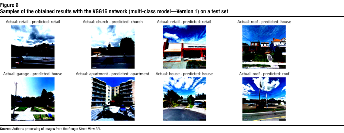
Description of figure 6
This figure shows multiple samples of street-view images of different buildings, and their actual and predicted types.Version 2
A second version of the multi-class model was trained with different parameters. In this model, the decay factor (on the learning rate) was set to 0.1 per 5 epochs. The number of epochs was set to 15, and cross-entropy loss was used in the training phase with weight decay of 10-3. We also eliminated the random cropping of the images (part of data augmentation), as it seemed to have a negative impact and randomly remove features from the images in the training set. This had an impact on the training accuracy. Furthermore, a dropout layer was introduced to the CNNs with a dropout probability of 0.15.
Figure 7 shows the learning curve for the training and validation phases for the trained CNNs (i.e., ResNet18, ResNet34, ResNet50 and VGG16) until 15 epochs. From the learning curves, one can see that all the CNNs converge by epoch 12. The best achieved training and validation accuracies for all the trained CNNs are also listed in Table 3. From the training accuracy curves and the results in the table, one can see that the best training accuracy was achieved with VGG16, where a training accuracy of 0.91 was obtained. Other CNNs achieved training accuracies ranging from 0.83 to 0.88. The best validation accuracy (0.74) was also achieved by VGG16, with ResNet34 and ResNet50 achieving a validation accuracy of 0.73. A considerable improvement (up to 5.7% increase over the first version) was obtained with the new parameters and data augmentation approach. However, there was also an increase in the training accuracy for all the CNNs (except ResNet50), despite the added dropout layer. The reason for the increase in training accuracy was the elimination of random cropping, as it could have randomly cropped distinctive features of the buildings.
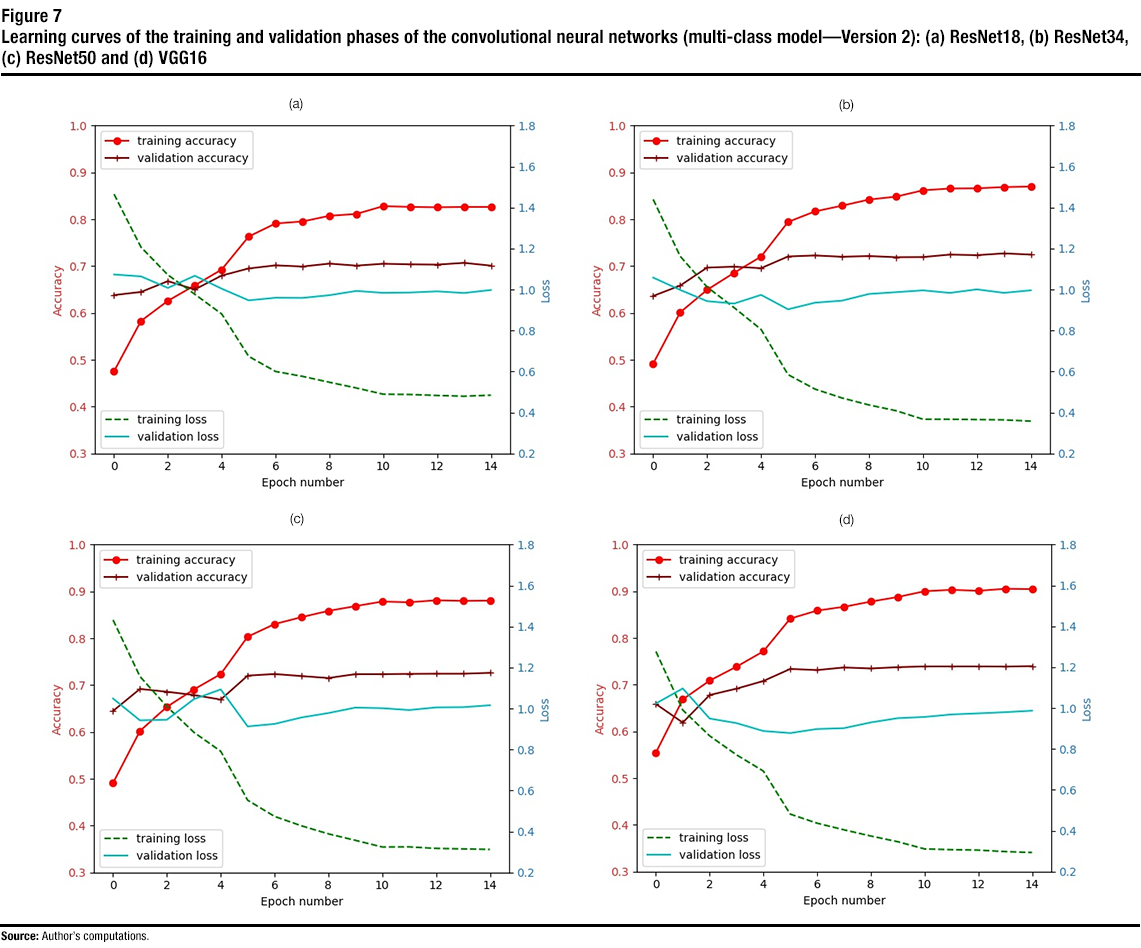
Description of figure 7
This figure contains four subfigures, each for a different architecture (e.g., ResNet18). Each subfigure shows the accuracy and loss versus the epoch number (for the training and validation phases) for the trained multi-class models (version 2). | Epoch number | ResNet18 | ResNet34 | ResNet50 | VGG16 | ||||||||||||
|---|---|---|---|---|---|---|---|---|---|---|---|---|---|---|---|---|
| training accuracy | validation accuracy | training loss | validation loss | training accuracy | validation accuracy | training loss | validation loss | training accuracy | validation accuracy | training loss | validation loss | training accuracy | validation accuracy | training loss | validation loss | |
| 1 | 0.475 | 0.638 | 1.466 | 1.074 | 0.492 | 0.636 | 1.440 | 1.058 | 0.491 | 0.645 | 1.433 | 1.049 | 0.555 | 0.659 | 1.277 | 1.023 |
| 2 | 0.583 | 0.645 | 1.207 | 1.064 | 0.601 | 0.658 | 1.163 | 0.998 | 0.602 | 0.692 | 1.157 | 0.942 | 0.669 | 0.619 | 0.990 | 1.096 |
| 3 | 0.626 | 0.668 | 1.072 | 1.008 | 0.649 | 0.697 | 1.012 | 0.943 | 0.654 | 0.686 | 1.010 | 0.946 | 0.709 | 0.678 | 0.864 | 0.949 |
| 4 | 0.659 | 0.650 | 0.977 | 1.067 | 0.686 | 0.699 | 0.912 | 0.932 | 0.691 | 0.679 | 0.885 | 1.046 | 0.739 | 0.692 | 0.771 | 0.927 |
| 5 | 0.693 | 0.680 | 0.881 | 1.004 | 0.720 | 0.696 | 0.805 | 0.974 | 0.724 | 0.669 | 0.791 | 1.093 | 0.771 | 0.708 | 0.692 | 0.888 |
| 6 | 0.763 | 0.695 | 0.674 | 0.947 | 0.794 | 0.721 | 0.585 | 0.904 | 0.803 | 0.720 | 0.553 | 0.913 | 0.842 | 0.734 | 0.481 | 0.878 |
| 7 | 0.791 | 0.702 | 0.600 | 0.960 | 0.817 | 0.723 | 0.514 | 0.936 | 0.830 | 0.724 | 0.474 | 0.925 | 0.859 | 0.731 | 0.437 | 0.898 |
| 8 | 0.795 | 0.699 | 0.576 | 0.959 | 0.829 | 0.720 | 0.471 | 0.946 | 0.845 | 0.719 | 0.428 | 0.957 | 0.867 | 0.737 | 0.404 | 0.902 |
| 9 | 0.808 | 0.705 | 0.548 | 0.973 | 0.842 | 0.722 | 0.437 | 0.978 | 0.859 | 0.715 | 0.388 | 0.978 | 0.878 | 0.735 | 0.374 | 0.930 |
| 10 | 0.811 | 0.701 | 0.520 | 0.993 | 0.848 | 0.719 | 0.409 | 0.987 | 0.869 | 0.723 | 0.357 | 1.005 | 0.888 | 0.738 | 0.346 | 0.951 |
| 11 | 0.828 | 0.705 | 0.489 | 0.984 | 0.862 | 0.719 | 0.367 | 0.996 | 0.879 | 0.723 | 0.324 | 1.002 | 0.900 | 0.739 | 0.311 | 0.957 |
| 12 | 0.827 | 0.704 | 0.488 | 0.986 | 0.866 | 0.725 | 0.367 | 0.984 | 0.877 | 0.724 | 0.325 | 0.993 | 0.903 | 0.739 | 0.307 | 0.969 |
| 13 | 0.826 | 0.703 | 0.483 | 0.991 | 0.866 | 0.723 | 0.365 | 1.001 | 0.881 | 0.724 | 0.318 | 1.006 | 0.901 | 0.739 | 0.305 | 0.974 |
| 14 | 0.826 | 0.707 | 0.479 | 0.983 | 0.869 | 0.727 | 0.364 | 0.984 | 0.880 | 0.724 | 0.315 | 1.007 | 0.905 | 0.739 | 0.298 | 0.980 |
| 15 | 0.826 | 0.701 | 0.485 | 0.998 | 0.870 | 0.725 | 0.358 | 0.996 | 0.880 | 0.726 | 0.312 | 1.016 | 0.905 | 0.740 | 0.293 | 0.987 |
| Architecture | Training accuracy | Validation accuracy |
|---|---|---|
| ResNet18 | 0.83 | 0.71 |
| ResNet34 | 0.87 | 0.73 |
| ResNet50 | 0.88 | 0.73 |
| VGG16 | 0.91 | 0.74 |
Version 3
A third version of the model was trained. Two modifications were implemented with the third model. First, the dataset was manually investigated to correct errors in data labelling. The images of each class were investigated to remove images that were there by mistake. Most of the cleaning was done on the “garage” and “roof” classes. The data for the garage class contained many images of houses (of which many did not even have a garage). The data for that class were cleaned to contain images of garages, or at least houses where a garage was apparent. For the roof class, the dataset is supposed to contain roof structures, such as the ones in gas stations or in front of hotels. However, the dataset for that class contained other images (houses, apartments, etc.). In addition to improving the labelling of the sets of images, the dropout probability for ResNet50 and VGG15 was set to 0.25.
For this version, we only show the highest values obtained for training and validation accuracies (Table 4). From the table, one can see that the best training accuracy was achieved with VGG16, where a training accuracy of 0.92 was achieved. The other CNNs achieved training accuracies ranging from 0.80 to 0.88. Because of the higher value of dropout probability used with ResNet50, its highest training accuracy is lower than that achieved with ResNet18 and ResNet34.
The best validation accuracy (0.78) was also achieved with VGG16, with the other CNNs achieving validation accuracy values between 0.75 and 0.77. This means that up to 11.4% increase is achieved over the first version. As one can see, a considerable improvement is achieved by cleaning the dataset. This is because cleaning removes images in the training or validation set that are mistakenly placed with the wrong class—these confuse the trained model and reduce its accuracy.
| Architecture | Training accuracy | Validation accuracy |
|---|---|---|
| ResNet18 | 0.85 | 0.75 |
| ResNet34 | 0.88 | 0.76 |
| ResNet50 | 0.80 | 0.77 |
| VGG16 | 0.92 | 0.78 |
Figure 8 shows the confusion matrices, as obtained on the validation dataset, of the third version of the finetuned CNNs. As one can see, the best classification accuracy is achieved on the house, garage and roof classes. This is because these classes have distinctive features. This also shows that the manual correction of the labelling significantly helped the model distinguish between the house and garage classes. The worst classification results were the ones for the retail and office building classes. Retail buildings have common features with other classes. For instance, they might be confused with the industrial (industrial buildings could have signs), roof (roofs mostly exist in gas stations with convenience stores) and apartment (stores may exist in the first floor) classes. Some office buildings may look like apartment buildings or have stores in the first floor, which may cause them to be classified as the aforementioned classes.
As previously mentioned, the benchmarking dataset contains a test set. The test set comprises 2,000 images collected from cities other than the cities in the training set. Version 3 of the VGG16 model was run on the test set, as that model provided the best validation accuracy. The classification accuracy achieved with VGG16 (Version 3) on this set was 0.69. This is a significant improvement (17%) in accuracy over that achieved with Version 1 and that achieved by (Kang et al., 2018).
Despite the positive results achieved, there is still room for improvement. By analyzing and optimizing the classes and the training set, the labelling of the training set may be further improved and achieve higher classification accuracy.
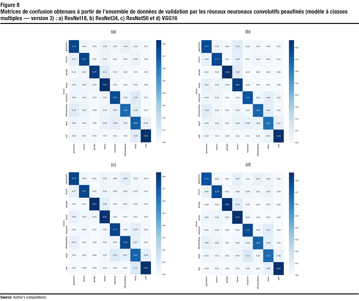
Description of figure 8
This figure shows the confusion matrices obtained on the validation set with the finetuned CNNs (multi-class model – version 3) for (a) ResNet18 (b) ResNet34 (c) ResNet50 (d) and VGG16. | Apartment | Church | Garage | House | Industrial | Office building | Retail | Roof | ||
|---|---|---|---|---|---|---|---|---|---|
| Actual (Resnet18) | Predicted (ResNet18) | ||||||||
| Apartment | 0.76 | 0.04 | 0.01 | 0.06 | 0.03 | 0.06 | 0.03 | 0.01 | |
| Church | 0.07 | 0.77 | 0.01 | 0.05 | 0.02 | 0.03 | 0.06 | 0 | |
| Garage | 0.02 | 0.04 | 0.79 | 0.11 | 0.02 | 0.02 | 0.01 | 0 | |
| House | 0.04 | 0.04 | 0.03 | 0.83 | 0.03 | 0.01 | 0.02 | 0 | |
| Industrial | 0.04 | 0.03 | 0.02 | 0.02 | 0.74 | 0.04 | 0.10 | 0.01 | |
| Office building | 0.10 | 0.05 | 0 | 0.05 | 0.06 | 0.64 | 0.08 | 0.01 | |
| Retail | 0.04 | 0.03 | 0 | 0.06 | 0.08 | 0.05 | 0.68 | 0.06 | |
| Roof | 0.03 | 0.02 | 0.01 | 0.01 | 0.01 | 0.01 | 0.09 | 0.82 | |
| Actual (Resnet34) | Predicted (Resnet34) | ||||||||
| Apartment | 0.77 | 0.04 | 0.02 | 0.10 | 0.02 | 0.03 | 0 | 0.01 | |
| Church | 0.05 | 0.77 | 0.01 | 0.80 | 0.01 | 0.03 | 0.02 | 0.01 | |
| Garage | 0.02 | 0.02 | 0.86 | 0.09 | 0 | 0 | 0 | 0 | |
| House | 0.07 | 0.04 | 0.04 | 0.82 | 0.02 | 0.01 | 0.01 | 0 | |
| Industrial | 0.04 | 0.04 | 0.01 | 0.02 | 0.74 | 0.03 | 0.09 | 0.03 | |
| Office building | 0.10 | 0.03 | 0.01 | 0.05 | 0.02 | 0.69 | 0.09 | 0.02 | |
| Retail | 0.05 | 0.05 | 0.01 | 0.06 | 0.06 | 0.06 | 0.65 | 0.07 | |
| Roof | 0.03 | 0.01 | 0 | 0.01 | 0.01 | 0.02 | 0.05 | 0.86 | |
| Actual (Resnet50) | Predicted (Resnet50) | ||||||||
| Apartment | 0.76 | 0.04 | 0.01 | 0.04 | 0.02 | 0.09 | 0.02 | 0.01 | |
| Church | 0.07 | 0.77 | 0.01 | 0.04 | 0.03 | 0.04 | 0.03 | 0.01 | |
| Garage | 0.01 | 0.01 | 0.83 | 0.08 | 0.02 | 0.03 | 0.02 | 0.01 | |
| House | 0.06 | 0.03 | 0.03 | 0.82 | 0.02 | 0.01 | 0.01 | 0.01 | |
| Industrial | 0.02 | 0.03 | 0.01 | 0.02 | 0.77 | 0.04 | 0.09 | 0.02 | |
| Office building | 0.07 | 0.02 | 0 | 0.02 | 0.04 | 0.76 | 0.07 | 0.02 | |
| Retail | 0.02 | 0.02 | 0 | 0.03 | 0.11 | 0.07 | 0.67 | 0.08 | |
| Roof | 0.01 | 0 | 0 | 0.01 | 0.01 | 0.01 | 0.12 | 0.83 | |
| Actual (VGG16) | Predicted (VGG16) | ||||||||
| Apartment | 0.76 | 0.03 | 0.01 | 0.07 | 0.02 | 0.07 | 0.04 | 0.01 | |
| Church | 0.06 | 0.78 | 0.01 | 0.04 | 0.04 | 0.02 | 0.05 | 0 | |
| Garage | 0 | 0 | 0.86 | 0.10 | 0.01 | 0 | 0.03 | 0 | |
| House | 0.03 | 0.04 | 0.03 | 0.87 | 0.02 | 0 | 0.01 | 0 | |
| Industrial | 0.02 | 0.04 | 0 | 0.02 | 0.78 | 0.04 | 0.10 | 0 | |
| Office building | 0.08 | 0.04 | 0.01 | 0.03 | 0.05 | 0.69 | 0.08 | 0.01 | |
| Retail | 0.03 | 0.03 | 0.01 | 0.04 | 0.12 | 0.03 | 0.67 | 0.06 | |
| Roof | 0 | 0.01 | 0 | 0.02 | 0.02 | 0.01 | 0.06 | 0.86 | |
5 Conclusion and future work
In this research, CNNs were finetuned to classify buildings into different types (e.g., house, apartment, industrial) using their street-view images. The CNNs use the structure of the façade in the building’s image for classification. Multiple state-of-the-art CNNs (e.g., ResNet50 and VGG16) were finetuned to classify buildings from their street-view images. The training and validation performance of the trained CNNs was measured and presented in this paper. Three versions of a multi-class model were trained and presented. In the first version, the CNNs were finetuned on a training set and evaluated on a separate validation set of street-view imagery. Validation accuracy of up to 0.7 (or 70%) was obtained with the first version of the model. A second version of the multi-class model was trained with all the networks on the same data set, but with further hyperparameter tuning and a different data augmentation approach. Validation accuracy of 0.74 or 74% (i.e., 5.7% improvement over the first version) was achieved with the second version of the model. Moreover, a third version of the model was trained with the same parameters of the second version, but on a dataset that was manually investigated to correct mislabelling of images. Even further improvement was achieved by the third version of the model. Validation accuracy of up to 0.78 or 78% (i.e., 11.4% improvement over the first version) was obtained with the third version of the model. In addition to the above, the models were evaluated on a test set of images that were taken from cities that are different from the ones in the training set. The results show that CNNs can be used to classify buildings from their street-view imagery, with classification accuracy of up to 0.78 (or 78%) on test images of buildings from the same cities in the training set, and an accuracy of up to 0.69 (or 69%) with test images from different cities. The results achieved with Version 3 of the model on the test set from different cities showed 17% increase in classification accuracy over that achieved with Version 1.
Despite the positive results, there is room for improvement to increase the classification accuracy of the models. Further work could be implemented to improve and restructure the datasets, and combine some of the similar classes (e.g., house and garage) to increase the accuracy of the models. Transfer learning could also be implemented to finetune and test the models on images that, in present application, were taken exclusively from one city in Canada. Additionally, the CNNs could be finetuned to produce different classification models that could be used to extract more properties of the buildings of interest (e.g., semi-detached house, row house). Moreover, an automatic system could be developed for joint image acquisition and classification with the trained models. Notably, the Google Street View Static API has limitations and terms of use. As a result, any models beyond the proof-of-concept level may require training with imagery obtained from a variety of different sources.
References
Al-Habashna, A. (2020). An open-source system for building-height estimation using street-view images, deep learning, and building footprints. Statistics Canada Articles and Reports, 18-001-X2020002. https://www150.statcan.gc.ca/n1/pub/18-001-x/18-001-x2020002-eng.htm
Al-Habashna, A. (2021). Building Height Estimation using Street-View Images, Deep-Learning, Contour Processing, and Geospatial Data. Proceedings - 2021 18th Conference on Robots and Vision, CRV 2021, 103–110.
Dong, S., Wang, P., & Abbas, K. (2021). A survey on deep learning and its applications. Computer Science Review, 40, 100379.
Gebru, T., Krause, J., Wang, Y., Chen, D., Deng, J., Aiden, E. L., & Fei-Fei, L. (2017). Using deep learning and google street view to estimate the demographic makeup of neighborhoods across the United States. Proceedings of the National Academy of Sciences of the United States of America, 114(50), 13108–13113.
Giri, C. (2016). Remote Sensing of Land Use and Land Cover. In Remote Sensing of Land Use and Land Cover. CRC Press. Retrieved from https://www.taylorfrancis.com/https://www.taylorfrancis.com/books/mono/10.1201/b11964/remote-sensing-land-use-land-cover-chandra-giri.
Google. (2020). Street View Static API. Retrieved from https://developers.google.com/maps/documentation/streetview/intro.
Grab Holdings. (2009). Open Street Cam. Retrieved from https://openstreetcam.org/map/@45.37744755572422,-75.65142697038783,18z.
He, K., Zhang, X., Ren, S., & Sun, J. (2016). Deep residual learning for image recognition. Proceedings of the IEEE Computer Society Conference on Computer Vision and Pattern Recognition, 2016-December, 770–778.
Kang, J., Körner, M., Wang, Y., Taubenböck, H., & Zhu, X. X. (2018). Building instance classification using street view images. ISPRS Journal of Photogrammetry and Remote Sensing, 145, 44–59.
Li, X., Zhang, C., & Li, W. (2017). Building block level urban land-use information retrieval based on Google Street View images. GIScience and Remote Sensing, 54(6), 819–835. https://www.tandfonline.com/doi/abs/10.1080/15481603.2017.1338389.
Mapillary. (2014). Mapillary. Retrieved from https://www.mapillary.com/.
OpenStreetMap. (2004). OpenStreetMap. Retrieved from https://www.openstreetmap.org/#map=4/30.56/-64.16.
PyTorch. (2016). PyTorch. Retrieved from https://pytorch.org/.
Quinn, J. et al. (2019). Dive Into Deep Learning: Tools for Engagement Paperback (1st ed.). Corwin.
Russakovsky, O., Deng, J., Su, H., Krause, J., Satheesh, S., Ma, S., Huang, Z., Karpathy, A., Khosla, A., Bernstein, M., Berg, A. C., & Fei-Fei, L. (2015). ImageNet Large Scale Visual Recognition Challenge. International Journal of Computer Vision, 115(3), 211–252. http://image-net.org/challenges/LSVRC/.
Simonyan, K., & Zisserman, A. (2015, September 4). Very deep convolutional networks for large-scale image recognition. 3rd International Conference on Learning Representations, ICLR 2015 - Conference Track Proceedings. Retrieved from http://www.robots.ox.ac.uk/.
Voulodimos, A., Doulamis, N., Doulamis, A., & Protopapadakis, E. (2018). Deep Learning for Computer Vision: A Brief Review. In Computational Intelligence and Neuroscience (Vol. 2018). Hindawi Limited.
- Date modified: