
Measuring proximity to services and amenities
An Open-source System for Building-height
Estimation using Street-view Images, Deep
Learning, and Building Footprints
by Ala’a Al-Habashna
Acknowledgments
The author of this paper would like to thank Dr. Alessandro Alasia for his valuable support, assistance, and input. The author would also like to thank the R&D Board of Statistics Canada for funding this project.
Summary
Deploying street-view imagery for information extraction has been increasingly considered recently by both industry and academia. Various efforts have been paid to extract information, relevant to various applications, from street-view images. This includes sidewalk detection in cities to help city planners and building instance classification. Building height is an important piece of information that can be extracted from street-view imagery. Such key information has various important applications such as economic analysis as well as developing 3D maps of cities. In this project, an open-source system is developed for automatic estimation of building height from street-view images using Deep Learning (DL), advanced image processing techniques, and geospatial data. Both street-view images and the needed geospatial data are becoming pervasive and available through multiple platforms. The goal of the developed system is to ultimately be used to enrich the Open Database of Buildings (ODB), that has been published by Statistics Canada, as a part of the Linkable Open Data Environment (LODE). In this paper, the developed system is explained. Furthermore, some of the obtained results for building-height estimation are presented. Some challenging cases and the scalability of the system are discussed as well.
1 Introduction
Building height is an important data to enhance economic analysis of (two dimensional) building footprints, which can be used for the analysis of urban development and urbanization processes, or to derive key socio-economic indicators on habitable or retail space. It can also be used to develop 3D maps of cities.
In the past, different technologies have been used for building height estimation such as Light Detection and Ranging (LiDAR) data (Sampath et al., 2010), as well as Synthetic Aperture Radar (SAR) (Brunner et al., 2010). LiDAR is a laser-based technology for measuring distances (Sampath et al., 2010). With this technology, laser light is illuminated on the target and the reflection is measured with a sensor. 3D representations of the area/objects of interest are built by measuring the differences in laser return times and wavelengths. SAR is a radar-based technology that is used for 3D reconstructions of objects or landscapes. With SAR, fine spatial resolution can be achieved using the motion of the radar antenna over the object/region of interest. The issue with the approaches above is that it is costly to obtain such data, which make their usability on a large scale infeasible.
Openly licensed street view imagery is spreading rapidly. Over the past few years, several platforms for street-view imagery have emerged, which offer different terms and conditions of services, and different degrees of "openness". Google Street-View (Google, 2020), Mapillary (Mapillary, 2014), and OpenStreetCam (Grab Holdings, 2009) are examples of such platforms. Such imagery provides remarkable opportunities to enrich existing data on buildings with complementary information relevant for further economic and spatial analyses. Furthermore, such imagery can be utilized on a large scale as they are largely available and easily accessible.
There has been some effort in the literature to extracting data from street-view images. This includes various applications such as estimating the demographic makeup of neighborhoods in the US (Gebru et al., 2017) to building instance classification (Kang et al., 2018). Results from the work above show that street-view images can indeed provide a rich source of information in multiple applications.
There is some work in the literature on using street-view images for building height estimation (Díaz et al., 2016; Yuan et al., 2016; Zhao et al., 2019). As mentioned above, the availability of this type of images makes them deployable on a large scale. Some of the work above use street-view images, while other use street-view images combined with building spatial information that can be obtained from 2D maps
In this paper, an algorithm for building height estimation is proposed. The approach is called Building Height Estimation using Deep Learning (DL) and Contour processing (BHEDC). BHEDC uses Convolutional Neural Networks (CNNs) for building detection in street-view images. Thereafter, various image processing techniques are used to extract the dimensions of the building in the image. The extracted information along with other spatial information (building corners, camera position, etc.) are used to estimate building height. The proposed approach was fully implemented using the Python programing language as well as open-source imagery and data. Results show that the proposed approach can be used for accurate estimation of building height from street view images.
The goal is to use the developed system to enrich 2D building footprints with building-height data. In 2019, Statistics Canada released the Open Database of Buildings (ODB) (Statistics Canada, 2019a) as part of an initiative to provide open micro data from municipal and provincial sources; the Linkable Open Data Environment (LODE) (Statistics Canada, 2019b). A first version of the ODB was followed by a second version released in collaboration with Microsoft, which resulted in a first mapping of virtually all building footprint across Canada. That 2D open database can now be improved and enhanced by adding attributes to building footprints and building height is among the most relevant pieces of information. For this reason, in 2020, Statistics Canada initiated this R&D project to explore the use of street-view imagery for building-height estimation.
In this paper, BHEDC and its implementation are presented in detail. The rest of the paper is organized as follows: Section 2 reviews the related work in the literature. Section 3 presents BHEDC and discusses the detection of buildings and extraction of their dimensions. Section 4 reviews the extraction of needed information from building footprint data. Section 5 presents the used camera-projection model for building height estimation. Section 6 discusses the obtained results and scalability of the system, and finally Section 7 states the conclusion and future work.
2 Background and related work
As mentioned in the previous section, street-view images have already been used for data extraction in multiple applications. In (Smith et al., 2013), machine learning and computer vision techniques were used to extract information about the presence and quality of sidewalks in cities. Local and global features including geometric context, presence of lanes, and pixel color were utilized with the random forest classifier to identify sidewalk segments in street view images. The results show that the proposed method can be used effectively for mapping and classifying sidewalks in street view images, which helps urban planners in creating pedestrian-friendly, sustainable cities.
In (Kang et al., 2018), a framework was proposed for classifying the functionality of individual buildings. The proposed approach classifies façade structures from a combination of street-view images and remote sensing images using CNNs. Furthermore, a benchmark dataset was created and used to train and evaluate the use of CNNs for building instance classification.
In (Lichao Mou, 2018), the authors address the problem of height estimation from a single monocular remote sensing image. A fully convolutional-deconvolutional network architecture was proposed and trained end-to-end, encompassing residual learning, to model the ambiguous mapping between monocular remote sensing images and height maps. The network is of a convolutional sub-network and deconvolutional sub-network, where the first part extract multidimensional feature representation and the second part uses the extracted feature to generate height map. A High-resolution aerial-image data set that covers an area of Berlin was used to train and test the proposed architecture. Despite the applicability of this approach, remote sensing images are not always available as open source on a large scale and for all areas.
There has been some work on using street-view images for building height estimation. In (Díaz et al., 2016), an algorithm is developed that acquires thousands of geo-referenced images from Google Street View using a representational state transfer system, and estimates their average height using single view metrology. Results show that the proposed algorithm can estimate an accurate average building height map of thousands of images using Google Street-View imagery. While such an algorithm estimates accurately the average height of buildings, there is a need to estimate the height of individual buildings.
In (Yuan et al., 2016), a method is proposed to integrate building footprints from 2D maps and street level images to estimate building height. From building footprints, the 2D geographic coordinates are obtained. The approach in (Yuan et al., 2016) is implemented by setting the elevation of the building footprint to the ground level, which gives 3D world coordinates. Then, camera projection is used to project the building footprint assuming the ground level. Afterwards, the elevation of the building footprint is increased incrementally until it is aligned with building roofline. At that point, the building height is estimated as the increased elevation.
In (Zhao et al., 2019), an algorithm has been proposed for building height estimation. In this algorithm, a street-view image is pre-processed. First, semantic segmentation is applied on the image for building recognition. Afterwards, Structured Forest (Dollar et al., 2013) (a machine learning approach for edge detection) is used to compute sketches of the buildings. From the grayscale-sketch images, building roofline is identified, and camera projection is used for height estimation
In this paper, an algorithm called BHEDC for building height estimation is proposed, that employs Google street-view images and building footprints which can be obtained from different sources (e.g., Open Street Map (OSM) (OpenStreetMap, 2004) or ODB (Statistics Canada, 2019a)). The proposed algorithm is similar to the last algorithm mentioned above in the sense that it utilizes semantic segmentation and roofline detection, for building height estimation. However, BHEDC eliminates the need for using machine learning for edge detection purposes. The proposed algorithm performs a series of image processing algorithms on the semantically segmented image for extracting building roofline. These methods include extraction of connected component, contours extraction and approximation, as well as other proposed algorithms.
The proposed algorithm is implemented completely with Python, which makes it possible to make it available as an open-source framework for building height estimation. A CNN was used for semantic segmentation of the input image. In the following sections, the proposed algorithm is discussed in further detail, and some of the obtained results are presented.
3 Building height estimation with BHEDC
In this section, a high-level view of how building height is estimated with BHEDC is presented. Afterwards, the extraction of building-dimension in the image is explained in more detail.
3.1 BHEDC algorithm: an overview
Figure 1 illustrates the process of building-height extraction with BHEDC. First, street-view image of the building of interest is downloaded. The Google Street-View Static API is used to obtain test imagery. The Street View Static API allows downloading static (non-interactive) street-view panorama or thumbnail with HTTP requests (Google, 2020). A standard HTTP request can be used to request the street-view image and a static image is returned. Several parameters can be provided with the request such as the camera pitch and the angle of view. After obtaining the image, DL-based semantic segmentation is applied to identify the building in the image.
Afterwards, a series of image-processing steps are implemented on the image to extract the height of the building in the image. Thereafter, building footprint data is obtained. In the current implementation, we get such data from OSM using HTTP requests. For this purpose, several available APIs (e.g., Nominatim and OSMPythonTools) are utilized. In future work, we will be updating the system to obtain this data from Statistics Canada’s ODB (Statistics Canada, 2019a). After obtaining all the needed building footprint data, computations are performed on the data and the camera location (obtained from a metafile that is downloaded with the street-view image) to estimate the distance between the camera and the building. Finally, the values obtained from the steps above are all used in the camera-projection model, to estimate the building height. In the following sections, the steps above are explained in more detail.
Figure 1
BHEDC: high level illustration of the workflow
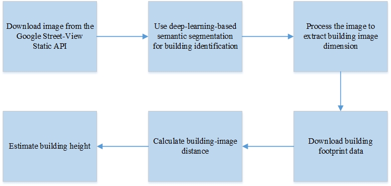
Description for Figure 1
This figure shows a flowchart that provides a high-level illustration of the BHEDC algorithm. There are 6 boxes in the flowchart. The first box contains the text “Download image from the Google Street-view Static API”. The second box contains the text “Use deep-learning-based sematic segmentation for building identification”. The third box contains the text “Process the image to extract building image dimension”. The fourth box contains the text “Download building footprint data”. The fifth box contains the text “Calculate building-image distance”. The sixth box contains the text “Estimate building height”.
3.2 Extracting building-image dimension
Here, the processes of extracting the building dimension in the image is discussed. In the next sections, acquisition of the needed geospatial information, as well as the deployment of all this information for building height estimation are explained.
Figure 2
Building-image dimension extraction BHEDC: high level illustration of the workflow

Description for Figure 2
This figure shows a flowchart that illustrates the process of building-image dimension extraction. There are 8 boxes in the flowchart. The first box contains the text “Use deep-learning-based semantic segmentation for building identification”. The second box contains the text “apply image thresholding to obtain pixels of the building in the image”. The third box contains the text “Extract the biggest connected component in the image”. The fourth box contains the text “Extract the contour”. The fifth box contains the text “Approximate the contour”. The sixth box contains the text “Get the highest points in the approximated contour”. The seventh box contains the text “Find the bottom line of the building”. The eighth box contains the text “Calculate the approximate building-image height”.
Measurements of the building in the image are needed to estimate the building actual height. This needs detection of the building in the image. Figure 2 illustrates the process of extracting the building-image height in the image with BHEDC. As shown in the figure, the process starts with applying semantic segmentation to identify the building in the image. Image segmentation partitions an image into multiple segments (Gonzalez et al., 2017). This technique is widely used in image processing as it simplifies further analysis and makes it possible to extract certain information. Grouping pixels together is done on the basis of specific characteristics such as intensity, color, or connectivity between pixels.
Semantic segmentation is a special type of image segmentation (Mottaghi et al., 2014). With semantic segmentation, a class is assigned to every pixel in the input image. This means that it is a classification problem. It is different from image classification where a label is assigned to the whole image. Semantic segmentation attempts to partition the image into meaningful parts and associate every pixel in an input image with a class label. For example, as in our case, it can be used to divide the pixels in the image to different classes (e.g., building, sky, or pedestrian). A very common application of semantic segmentation is self-driving vehicles. Nowadays, deep neural networks are usually used to solve semantic segmentation problems. In particular, CNNs achieve great results in terms of accuracy and efficiency. CNNs is a class of deep neural networks, most commonly applied to analyzing visual imagery. A CNN consists of an input and an output layers, as well as multiple hidden layers. The hidden layers of a CNN typically consist of a series of convolutional layers that convolve with a multiplication or other dot product. A TensorFlow-based CNN is used for semantic segmentation of the street view images (Chen et al., 2018). The employed architecture (xception-71) (Chen et al., 2018) is an improved version of the original Xception model (Chollet, 2017) with the following improvements: (1) more layers, (2) all max pooling operations are replaced by depth-wise separable convolution with striding (this allows the application of atrous separable convolution for feature maps extraction at an arbitrary resolution), and (3) extra batch-norm and ReLU after each 3x3 depth-wise convolution are added (Chen et al., 2018).
The original Xception architecture (stands for “Extreme Inception”) (Chollet, 2017) is based entirely on depth-wise separable convolution layers. It is a linear stack of Depth-wise separable convolution layers with residual connections. This simplify the definition and modification of the architecture. Promising image classification results with fast computations have been achieved with this model on ImageNet, and that is the reason of it is adoption for semantic segmentation in (Chen et al., 2018). The model in (Chen et al., 2018) was adopted here after testing multiple architectures for semantic segmentation and it found to give the best and more reliable segmentation results. It is worth mentioning that the used model was trained on images from European cities (Cityscapes dataset), and we aim to perform transfer learning. However, throughout testing the model with many images of buildings in the city of Ottawa, Canada, it seems that the features learned on buildings from European cities work well on buildings from Ottawa as well.
After downloading the image using a Python client, the image is fed to the CNN. The output is a semantically segmented image with the pixels labeled to multiple classes (e.g., sky, building, or street). Figure 3 shows an example of a sample image for a commercial building in Ottawa, Canada, that is downloaded with the Python client from the Google Street-View Static API, using HTTP request. Figure 4 shows the output of the CNN, which is a semantically segmented image.
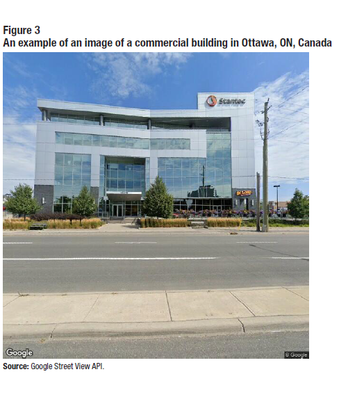
Description for Figure 3
This figure shows a sample test image of a commercial building in Ottawa, ON, Canada.
As can be seen in Figure 4, the building shows up as green subregions in the output image. Due to imperfections in the CNN, there might be other small green subregions in the image, as can be seen in Figure 4. Afterwards, thresholding is applied to the image in Figure 4, to extract only the pixels that represents the building. The output image of thresholding is a binary image, with white pixels (building pixels) on a black background. As mentioned above, the image might contain other small subregions. These could be a result of imperfection of the semantic segmentation, or a result of another far building in the background. To eliminate these irrelative subregions, the largest connected component in the image is extracted. The output of this step is one white region in the image (the building), superimposed on a black background, as can be seen in Figure 5.
The next step would be to extract the border of the building. For this goal, the contour of the foreground of the image (the building) is extracted. Contours are simply a curve connecting the continuous points (along the boundary) of a shape in the image. Contours are widely used and very useful for shape analysis and object detection and recognition.

Description for Figure 4
This figure shows the output image from the Convolutional Neural Network, with the image in figure 3 as the input. The output of the Convolutional Neural Network shown in the figure is the semantically segmented image. The image is divided into multiple subregions, where each subregion belongs to a certain class (e.g., building, road, vegetation, etc.) and has a unique color. The building shows in the image as a green subregion. Vegetation subregions are marked with purple. The road shows in the image as a black subregion.

Description for Figure 5
This figure shows a binary image which is the output of image thresholding and connected component extraction with the image in figure 4 as the input. The image in the figure is a black and white image with the white region representing the building pixels.
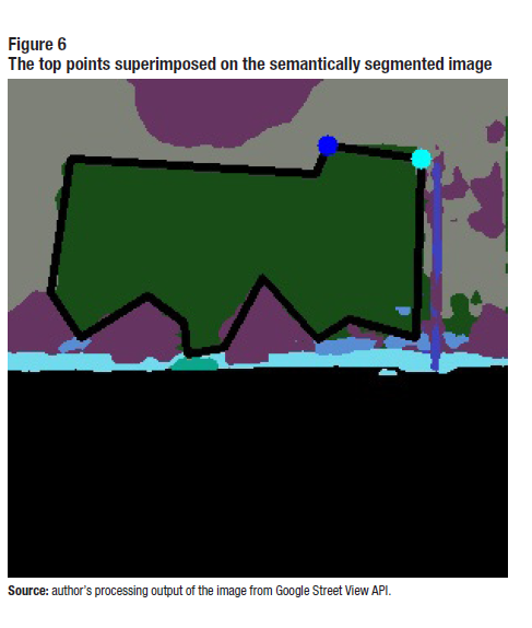
Description for Figure 6
This figure shows the semantically segmented image (the output of the Convolutional Neural Network) with the top two points of the contour superimposed on it.
The goal here is to extract the top line of the building in the image. To do that, the extracted contour is approximated. Instead of having a contour comprising of many points along the boundary of the foreground/building, an approximated contour is generated that contains the main corners of the foreground. The degree by which the contour is approximated can be controlled. After extracting the approximated contour of the building in the image, the top two points of the approximated contour are extracted. These two points give the roofline of the building in the image. Figure 6 shows the extracted top points of the building’s approximated contour superimposed on the building in the semantically segmented image.
As will be explained later, the lowest point of the building that is at or above the horizontal midline of the image needs to be detected. For that purpose, a simple algorithm is proposed and implemented, that scans the image, starting from mid-horizontal line looking for pixels of the connected component. When this is found by the algorithm, the height of the building in the image is considered as the height from the lowest line containing a connected-component pixel, to the roofline.
Figure 6. and Figure 7. show the results obtained for the same steps with a residential building in Ottawa, ON, Canada.
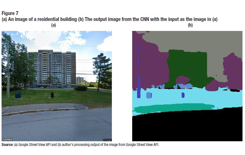
Description for Figure 7
(a) This figure shows a sample test image of a residential building in Ottawa, ON, Canada. (b) This figure shows the output image from the Convolutional Neural Network, with the image in figure 7-a as the input. The image in 7-b is divided into multiple subregions, where each subregion belongs to a certain class (e.g., building, road, vegetation, etc.) and has a unique color. The building shows in the image as a green subregion. Vegetation subregions are marked with purple. The road shows in the image as a black subregion.

Description for Figure 8
(a) The output of image thresholding and connected component extraction of the image in Figure 7-b. The image in Figure 8-a is a black and white image with the white region represents the building pixels. (b) This figure shows the semantically segmented image (the output of the Convolutional Neural Network) with the top two points of the contour superimposed on it.
4 Using building footprint data
In addition to building identification and extraction of the building dimension in the image, we need to identify the location of the building and the camera and compute the distance between them. This is needed in the camera projection model to estimate the building height. To get information about the building location, OSM (OpenStreetMap, 2004; Wikipedia, 2004) is utilized. OSM is platform that provides a free editable map of the world. It has many use cases such as generation of maps, geocoding of address and place names, and route planning (OpenStreetMap, 2004; Wikipedia, 2004).
In our case, OSM is used for (1) geocoding, i.e., getting the latitude/longitude from an input text, such as an address or the name of a place, and reverse geocoding, i.e., converting geographic coordinates to a description of a location, usually the name of a place or an addressable location. OSM is also used to (2) obtain building footprints, which includes various spatial data on the building of interest. In future work, we will be updating the system to obtain this data from Statistics Canada’s ODB (Statistics Canada, 2019a). Such data can be available locally which speeds up the operation of the system.
Nominatim is a tool to search OSM data by the name and address (geocoding) and to generate addresses of OSM points (reverse geocoding). Python is used to access this API via HTTP requests. First, a request is made to get the location of the building. The returned location object contains various pieces of information such as the latitude, longitude, type of the record (way, node, etc.), and the OSM Id of the record. Afterwards, the OSMPythonTools API is used to obtain the building footprint using the OSM Id.

Description for Figure 9
(a) This figure shows a screenshot of the map of a building and its border as viewed in Open Street Map (b) This figure shows the map of the building with one of the nodes of the building highlighted.
The building footprint comprises of important data such as the latitude/longitude for the center of the building, and the latitude/longitude of different nodes of the building, i.e., various points on the border of the building, as can be seen in Figure 9. Once the nodes of the building are obtained, a list of these nodes is built, and the building is treated as a polygon. Then, the location of the camera is requested from a metadata file that is downloaded from the Google Street-View API with the image request, and the distance between the camera and the building is calculated.
5 Camera-projection model
A camera-projection model specifies mathematically the relationship between the coordinates of a point in three-dimensional space and its projection onto another plane. It is used to model the geometry of projection of 3D points, curves, and surfaces onto a 2D surface (e.g., view plane, image plane, etc.). After extracting all the information above, the camera projection model is used to estimate the actual height of the building. The same camera-projection model in (Zhao et al., 2019) is used here. In this section, the camera-projection model used for building height estimation is briefly explained.
Let us start by defining two coordinate systems. The first one is the camera coordinate system, referred to by , where denotes the origin point of that system.
The second system is the image-plane coordinate system, referred to by , where denotes the origin point of that system. Both coordinate systems are shown in Figure 10.
Figure 10
Illustration of the camera-projection model

Description for Figure 10
The figure shows an Illustration of the camera-projection model. The figure shows a rectangular prism that represents the building. The camera is positioned at a distance from the building. A 3-diminational coordinate system is shown above the camera which represents the camera coordinate system. Behind the camera is two-dimensional plane which represents the image plane, with a two-dimensional coordinate system superimposed on it. The building image height in the image plane, , is used with the distance, , along with other parameters in the camera projection model to estimate the building height .
As can be seen in the figure, is the actual building height. Let denote the estimated building height, and is the distance between the camera and the building. Furthermore, let denotes the height of the camera, which is the height of the person holding the camera or the height of the car where the camera is mounted (can be assumed as constant). The estimated building height in this case can be given as,
where is the building-image height above the mid-horizontal line of the image, and is the focal length of the camera.
6 Results
6.1 Obtained results and analysis
In this section, some of the obtained results from the developed system for building height estimation are presented and discussed. The developed system was tested on various buildings (commercial and residential) in the city of Ottawa, Canada. A random set of 20 buildings were considered. The minimum height in the set is 4m and the maximum height is 54m. Over 50% of the buildings in the set are higher than 14m. All the images where downloaded with spatial resolution of 640×640. The images where fed to the system without cropping or augmentation. In this section, we show some samples of the obtained results. We also analyze the obtained results and evaluate the performance of the system in terms of estimation error (based on the data set from Ottawa).
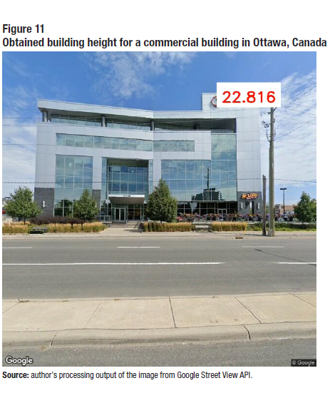
Description for Figure 11
This figure shows an image of a commercial building in Ottawa, Canada, with the estimated building height printed on top of the building.
Figure 11 shows the result obtained for a commercial building in Ottawa, Canada. The result is plotted on top of the building as shown in the figure. As can be seen, the estimated height for this building is 22.83m, and the actual height for the building is about 20m.

Description for Figure 12
This figure shows two images of residential buildings in Ottawa, Canada, with the estimated building heights printed on top of the buildings.
Figure 12 shows more results obtained from 2 different residential buildings in Ottawa, Canada. The actual height for the building in Figure 12-a is 45m, and the figure show that the result obtained for that building is 48.052m. Regarding the building in Figure 12-b, the actual height is 42m, and the figure shows that the estimated height is 44.044m.
As mentioned above, the developed system was tested on various buildings (commercial and residential) in the city of Ottawa, Canada. A random set of 20 buildings were considered. The building height was estimated for all the sample buildings, and the estimation error was calculated. The average estimation error from all the samples is 2.32m.
Figure 13 shows the Empirical Cumulative Distribution Function (ECDF) for the estimation errors. The ECDF shows that 50% of the buildings have and estimation error less than or equal to 2m, and that 85% of the buildings have estimations errors of 4m or less.
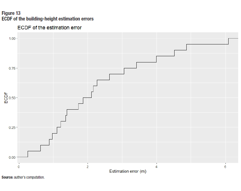
Description for Figure 13
This figure shows the Empirical Cumulative Distribution Function of the building-height estimation errors.
6.2 Challenging cases
Currently, the system is being improved to handle some challenging cases. For one, vegetation sometimes might make it difficult to detect the bottom edge of the building as can be seen in Figure 14. This is not a problem in many cases as we need the bottom of the building that is at or above the mid-horizontal line of the image. Another challenging case is when the camera is facing a corner of the building rather than one of the facades of the building.
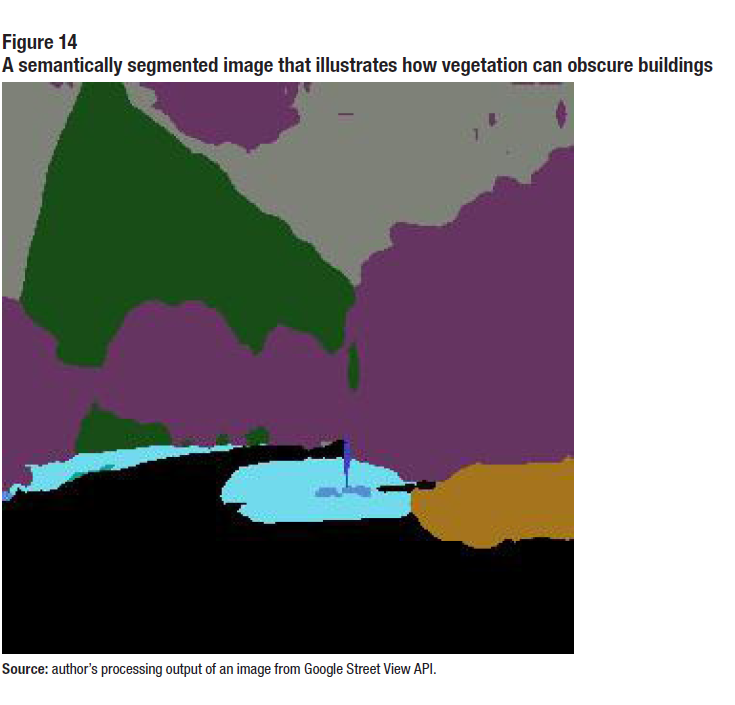
Description for Figure 14
This figure shows a semantically segmented image that illustrates how vegetation can obscure a building and cause difficulty in building identification.
6.3 Scalability of the developed system
When it comes to the scalability of the system, there are two main concerns, i.e., cost and execution time. Currently, it takes about 30 seconds to estimate the height of a building, on a quad-core Intel i7 processor with 16G of RAM. Of course, this can be speedup by using a more powerful machine or by running the system on the cloud. To the best of the author’s knowledge, available commercial solutions charge approximately in the order of US $7 per 1000-image requests. It is also worth mentioning that each platform may be subject to specific terms and conditions. As illustrative examples, we show two study cases here for the scalability of the system: the city of Toronto and the city of Ottawa. According to (Emporis, 2000), there are 9,538 buildings in the city of Toronto (commercial, government, halls, stadiums). To generate the building height for these buildings with the developed system (based on the measurements above), it will take about 79.5 hours and cost about US $10. The same source (Emporis, 2000), states that in the city of Ottawa, Canada, there are 935 buildings (commercial, government, halls, stadiums). To generate the building height for these buildings with the developed system (based on the measurements above), it will take about 7.8 hours and cost less than US $7.
7 Conclusion
Recently, there has been an increasing interest in using street-view imagery to extract important information relevant to many applications. An example of such efforts is employing street-view images to detect and map sidewalks and traffic signs in cities to help city planners. Building height is an important piece of information that can be extracted from street-view imagery. Such key information has various important applications such as economic analysis as well as developing 3D maps of cities. In this project, an open-source system is developed for automatic estimation of building height from street-view images using Deep Learning (DL), advanced image processing techniques, and geospatial data. Both street-view images and the needed geospatial data are becoming pervasive and available through multiple platforms. The goal of the developed system is to ultimately be used to enrich the Open Database of Buildings (ODB), that has been published by Statistics Canada, as a part of the Linkable Open Data Environment (LODE). The developed system was tested on a group of residential and commercial buildings in Ottawa, Canada. The obtained results show that the system can be used to provide accurate building-height estimation. Furthermore, scalability analysis shows that the system can be utilized for building-height estimation on a larger scale (e.g., at the level of a big city or a country). The system is currently being improved to handle more cases (e.g., process images taken with high camera elevation angle, automatic camera elevation angle selection, etc.). Furthermore, more testing will be implemented on the system to evaluate its performance with bigger data set and with images from different areas (e.g., bigger cities with denser areas).
References
Brunner, D., Lemoine, G., Bruzzone, L., & Greidanus, H. (2010). Building height retrieval from VHR SAR imagery based on an iterative simulation and matching technique. IEEE Transactions on Geoscience and Remote Sensing, 48(3 PART2), 1487–1504.
Chen, L.-C., Zhu, Y., Papandreou, G., Schroff, F., & Adam, H. (2018). Encoder-decoder with atrous separable convolution for semantic image segmentation. European Conference on Computer Vision, 833–851.
Chollet, F. (2017). Xception: Deep learning with depthwise separable convolutions. Proceedings - 30th IEEE Conference on Computer Vision and Pattern Recognition, CVPR 2017, 1800–1807.
Díaz, E., & Arguello, H. (2016). An algorithm to estimate building heights from Google street-view imagery using single view metrology across a representational state transfer system. Dimensional Optical Metrology and Inspection for Practical Applications V, 1–8.
Dollar, P., & Zitnick, C. L. (2013). Structured forests for fast edge detection. Proceedings of the IEEE International Conference on Computer Vision, 1841–1848.
Emporis. (2000). EMPORIS. Retrieved from https://www.emporis.com/
Gebru, T., Krause, J., Wang, Y., Chen, D., Deng, J., Aiden, E. L., & Fei-Fei, L. (2017). Using deep learning and google street view to estimate the demographic makeup of neighborhoods across the United States. Proceedings of the National Academy of Sciences of the United States of America, 114(50), 13108–13113.
Gonzalez, R., & Woods, R. (2017). Digital image processing (4th ed.). Pearson.
Google. (2020). Street View Static API. Retrieved from |https://developers.google.com/maps/documentation/streetview/intro
Grab Holdings. (2009). Open Street Cam. Retrieved from https://openstreetcam.org/map/@45.37744755572422,-75.65142697038783,18z
Kang, J., Körner, M., Wang, Y., Taubenböck, H., & Zhu, X. X. (2018). Building instance classification using street view images. ISPRS Journal of Photogrammetry and Remote Sensing, 145, 44–59.
Lichao Mou, X. X. Z. (2018). IM2HEIGHT: Height estimation from single monocular imagery via fully residual convolutional-deconvolutional network. ArXiv Preprint, ArXiv:1802.10249.
Mapillary. (2014). Mapillary. Retrieved from https://www.mapillary.com/
Mottaghi, R., Chen, X., Liu, X., Cho, N. G., Lee, S. W., Fidler, S., Urtasun, R., & Yuille, A. (2014). The role of context for object detection and semantic segmentation in the wild. Proceedings of the IEEE Computer Society Conference on Computer Vision and Pattern Recognition, 891–898.
OpenStreetMap. (2004). OpenStreetMap. Retrieved from https://www.openstreetmap.org/#map=4/30.56/-64.16
Sampath, A., & Shan, J. (2010). Segmentation and reconstruction of polyhedral building roofs from aerial lidar point clouds. IEEE Transactions on Geoscience and Remote Sensing, 48(3 PART2), 1554–1567.
Smith, V., Malik, J., & Culler, D. (2013). Classification of sidewalks in street view images. 2013 International Green Computing Conference Proceedings, IGCC 2013, 1–6.
Statistics Canada. (2019a). Open Database of Buildings. Retrieved from https://www.statcan.gc.ca/eng/lode/databases/odb
Statistics Canada. (2019b). The Linkable Open Data Environment. Retrieved from https://www.statcan.gc.ca/eng/lode
Wikipedia. (2004). OpenStreetMap. Retrieved from https://en.wikipedia.org/wiki/OpenStreetMap
Yuan, J., & Cheriyadat, A. M. (2016). Combining maps and street level images for building height and facade estimation. Proceedings of the 2nd ACM SIGSPATIAL Workshop on Smart Cities and Urban Analytics, UrbanGIS 2016, 1–8.
Zhao, Y., Qi, J., & Zhang, R. (2019). CBHE: Corner-based building height estimation for complex street scene images. Proceedings of the World Wide Web Conference, 2436–2447.
- Date modified: