
Reports on Special Business Projects
Measuring proximity to services and amenities: An experimental set of indicators for neighbourhoods and localities
by Alessandro Alasia, Nick Newstead, Joseph Kuchar and Marian Radulescu
Acknowledgments
This project was initiated and funded by the Canada Mortgage and Housing Corporation (CMHC). The support of this organization and its staff is gratefully acknowledged. In particular, Jean-Philippe Deschamps-Laporte (during the first years of the project), Stephanie L. Shewchuk, and George A. Ngoundjou Nkwinkeum provided continuous guidance and valuable feedback for the implementation of this project. At Statistics Canada several other people contributed to the completion of this work; Jean Le Moullec managed the first phase of the project and provided critical inputs. Research assistance was provided by Marina Smailes. The Digital Innovation Team of Statistics Canada, specifically Marc-Philippe St. Amour and Jean-Philippe Tissot, as well as the Cloud Project Team (Francis Mailhot) were instrumental in supporting access to the necessary IT tools for the analysis.
Executive summary
In a highly connected and networked world, the significance of geography has unquestionably changed. Nevertheless, the relevance of space, as measured by physical proximity, for economic and social outcomes has not disappeared. Spatial proximity to service and amenities remains a driver of socioeconomic outcomes for business and people alike. Moreover, the COVID-19 pandemic has highlighted the importance of such information, not only for crisis management and emergency response purposes, but also for the population at large.
To account for proximity to service and amenities, national and local policymakers need measures that are as granular as possible and comparable across jurisdictions. In Canada, this type of measurement framework for proximity in support of policy and planning was lacking. To fill this gap and support the National Housing Strategy’s social inclusion pillar, Statistics Canada collaborated with the Canada Mortgage and Housing Corporation (CMHC) for the implementation of a set of proximity measures to services and amenities. The result of this collaboration is the first national Proximity Measure Database (PMD), which is now released to the public.
This paper presents the methodology used to generate the first nationwide database of proximity measures and the results obtained with a first set of ten measures. The computational methods are presented as a generalizable model due to the fact that it is now possible to apply similar methods to a multitude of other services or amenities, in a variety of alternative specifications.
Due to the scale of this project, the implementation of these measures required various innovative solutions. Specifically, the computational methods are largely reliant on open source software and were implemented in a cloud environment and some of the measures are entirely based on newly developed databases of open and publicly available data.
Currently, the PMD contains proximity measures for ten distinct services and amenities. These services and amenities include employment, grocery stores, pharmacies, health care, child care, primary education, secondary education, public transit, neighbourhood parks, and libraries. In addition to these, a composite indicator of selected measures has also been included to quantify general availability of services and amenities.
All measures are provided at the level of the dissemination block (DB), which corresponds to a city block in urban areas or an area bounded by roads or other natural features in rural areas. The entirety of Canada is subdivided into approximately half a million DBs. This is the smallest standard geography offered by Statistics Canada, and therefore, provides the highest geographic resolution currently possible. Coverage for some measures that have been included in the database varies based on availability of authoritative open data sources. As the number of authoritative open data sources increases, a trend in recent years, future iterations of the proximity measures will have more comprehensive coverage spatially.
Proximity measures are based on a gravity model that accounts for the distance between a reference dissemination block (DB) and all the DBs within a given distance in which the service is available. The proximity measures also take into account the size of services, and the presence of services in the reference DB.
All measures, except public transit, are based on either walking or driving network distances between the centroids of dissemination blocks (as opposed to straight-line distances). For public transit, the walking network distance is between the centre of a dissemination block and any public transit stop within a given distance. The size of the service is captured by total employment or total revenue of the service, or more simply, the presence of points of access to the service within a given distance. The measure of size of the service is specific to each measure.
The proximity measures are released as a normalized index value, meaning that the values resulting from computations were converted to a scale from 0 to 1, where 0 indicates the lowest proximity and 1 the highest proximity in Canada. The values are normalized at the national level in order to retain as much detail as possible.
Using the specifications (type of service, distances, and weights) required by CMHC, the main aggregate results can be summarized as follows.
- Approximately 20% of Canadians are living in “amenity dense” neighbourhoods. Amenity dense neighbourhoods meet the following criteria: access to at least one grocery store, pharmacy, and public transit stop within 1 km walking distance, a child care facility, primary school, and library within 1.5 km walking distance, a health facility within 3 km driving distance, and employment within 10 km driving distance.
- Nearly half of Canadians live in a neighbourhood or locality within 1 km walking distance from a grocery store. In larger metropolitan areas, 55% of population live in proximity to a grocery store; this percentage drops to 30% for those living in smaller metro areas and to 16% for the population living in rural areas.
- Nearly 60% of Canadians live in neighbourhoods or localities that are within 1 km walking distance from a pharmacy. Roughly 88% of Canadians live in neighbourhoods or localities that are within 3 km driving distance from a health care facility. This figure is 97% for those living in large metropolitan areas, 87% for those living in smaller metropolitan areas, and roughly 50% for those living in rural areas.
- Roughly 70% of Canadians live in neighbourhoods or localities that are within 1.5 km walking distance from primary education services – a similar figure also applies for child care services. This percentage is not as high for secondary schools. Roughly 42% of Canadians live within 1.5 km walking distance from a secondary school. This figure is 49% for those living in larger metropolitan areas, 38% for those living in smaller metropolitan areas and less than 20% for those in rural areas.
- Public transit services are typical of metropolitan areas. In large metropolitan areas of Canada, nearly 90% of the population lives within 1 km walking distance to a public transit stop. British Columbia, Quebec and Alberta have the highest percentage of their metropolitan population living in proximity (1 km walking distance) to a transit stop. British Columbia is the only province in which a high share of residents of smaller metropolitan areas (about 70%), and residents in rural areas (nearly 20%) enjoy proximity of a transit stop within 1 km walking distance.
- Roughly 75% of Canadians live in neighbourhoods or localities that are within 1 km walking distance of neighbourhood parks. In general, this number is higher in larger metropolitan areas, but there is significant variance between provinces. For example, Newfoundland and Labrador and New Brunswick both have about 50% or less of their metropolitan population in proximity of this amenity. In contrast, a relatively large share of rural residents of Quebec and British Columbia (about or slightly more than 20%) enjoy proximity to neighbourhood parks.
- Roughly 30% of Canadians live within 1.5 km walking distance to a library. This figure is relatively similar across regions – 33% in larger metropolitan areas, 22% in rural areas.
While these aggregate figures provide key insights, the real power of the work presented in this paper lies in the availability and visualization of these measures at the dissemination block level for all of Canada. The Proximity Measures Data Viewer developed for this analysis provides ready access to the level of granular geographic information that is needed for these measures: Proximity Measures Data Viewer.
The methodological and data framework developed for this analysis, which includes a database of 2.6 billion point-to-point distances, can now be adapted for the computation of a variety of alternative specifications of the same measures or additional measures of proximity to other services and amenities, in response to and in support of a variety of planning and policy needs.
Introduction
Recent literature has highlighted the persistent relevance of physical proximity and location in an increasingly digital economy, often perceived as spaceless (OECD 2019). Even in a world that is rapidly shifting toward digital technologies, evidence has shown that physical proximity between entities, social and economic actors, or consumers and providers of a service, remains a relevant driver of socioeconomic outcomes.
Physical proximity to services and amenities has a determinant contribution to economic performances of businesses, quality of life for individuals, and location decisions for people and businesses alike. For individuals, having physical access to basic services and amenities is a key determinant of social inclusion, their capacity to meet basic needs, and their ability to fully participate in social and economic development. The provision of some degree of services and amenities for all neighbourhoods is crucial for cities to attain social and economic sustainability at the local level.
In order to establish a measurement framework for proximity to services and amenities, Statistics Canada partnered with the Canada Mortgage and Housing Corporation (CMHC). CMHC is leading the implementation of a National Housing Strategy, which over the next ten years is expected to enable large investments in strengthening the quality of housing and neighbourhoods across Canada.Note Physical proximity to services and amenities is considered a relevant component of a broader notion of accessibility, which, in turn, is a pillar of social inclusion. These concepts are increasingly embedded in municipal planning and urban design. Municipalities, in Canada and internationally, are starting to make explicit reference to the concept of a “15-minute-neighbourhood” in their urban development plans; that is a neighbourhood in which essential services or those typically accessed on a daily basis can be reached within a 15-minute walk from one’s doorstep. Note
The collaboration between Statistics Canada and CMHC resulted in the release of the first nationwide Proximity Measures Database (PMD). This database, along with a visualization tool that shows the spatial distribution of the proximity measures, was made public as an early release in response to the urgent data needs to address the COVID-19 crisis.
This paper details the methods used in the development of the Proximity Measures Database. The approach used for this purpose filled an existing measurement gap by providing proximity measures at the level of localities or neighbourhoods, using the highest possible level of geographic granularity, while maintaining comparability across Canada.
Most importantly, the methods used for the PMD are based on a generalizable model that has considerable potential for extensions and adaptations, as well as applications for several other services or amenities. For this reason, the emphasis of this paper is on methodological aspects, rather than the analysis of the ten proximity measures generated in this first iteration of the PMD. One of the aims of this paper is to stimulate feedback from stakeholders, in view of further methodological improvements of the measures as well as updates of the measures when new data sources become available.
The paper is organized into six sections. This introductory section highlights the nature of the measurement gap and the innovations that were required to close the gap. Section 2 presents a general computation model, which is the foundational conceptual model that underpins all measures presented in this paper. Section 3 discusses the data sources, highlighting the potential of integrating open data with official statistical sources. Section 4 details the implementation methods. Section 5 discusses the specification of the ten measures. Section 6 presents the results for the first set of proximity measures developed for CMHC. The paper concludes with considerations for further developments.Understanding the measurement gap
In the social sciences literature, there is abundant evidence indicating that the degree of physical proximity determines socioeconomic outcomes and behaviours. In the economic literature (Melo, et al. 2017) showed that agglomeration externalities - the benefit in cost reductions and gains in efficiency that result from proximity among economic agents, occur primarily in a short distance radius while remaining small at wider distances. Marketing analysis suggests that geographic proximity has become increasingly important with a growing number of marketing services that use the geographic locations of consumers (Becker et al. 2017). Along similar lines, behavioural studies have shown that despite the growing use and impact of social media, proximity among individuals remains a key determinant of the likelihood to engage in friendships (Nguyen and Szymanski 2012).
For these reasons, it is not surprising that the methodological research on proximity measurement has also flourished, in different disciplinary domains and under the different headings of proximity, accessibility, and remoteness (OECD 2013, OECD 2018).Note Alasia et al. 2017 provided a summary of this literature, with a focus on remoteness and accessibility, while further literature review was undertaken in preparation for this analysis.
There are two main insights that emerged from these literature reviews. On one hand, the diversity of conceptual and methodological approaches with no single or predominantly accepted definition; on the other hand, the operational challenges that limited the development of a comprehensive measurement framework. The implementation of a comprehensive measurement framework for proximity was limited by data coverage, or the availability of computational capacity for relatively complex network analysis.
The paucity of data with precise geolocation of amenities and services, the lack of full coverage, and the difficulty of obtaining appropriate data to measure the location of economic activities has been lamented in the literature (Head and Mayer 2004) (Duranton and Kerr 2015). Similarly, the computational capacity to process even relatively simple network analyses, when the order of magnitude of network links is in the billions, has been until recently a major operational challenge.
The consequences of these limitations have been threefold. First, measures of proximity or accessibility were developed for limited geographic areas, such as for instance selected metropolitan regions (see Apparicio and Séguin 2006). Second, measures that were developed with broad national coverage were based on relatively large territorial units (e.g., regions or major metro areas), with substantial loss of geographic granularity (see OECD 2013). Third, attempts to reach broad coverage and high geographic granularity has often had to compromise on methods, for instance using less computationally demanding methods to determine distance to services, such as “as-the-crow-flies” distance measurements to a single point of service provision (see OECD 2013). The expansion of computational capacity combined with improving geocoding of official statistics and emerging new sources of geocoded microdata has now made this type of analysis possible.Innovation elements that moved us forward
Against the backdrop described in the previous section, three elements of innovation have made this analysis possible with realistic timeframes and attainable costs: the expansion of computational capacity through the use of cloud computing, the improving geocoding of official statistics and emerging new sources of geocoded microdata, as well as an extensive use of open-source software and analytical tools.
Data processing power required to generate neighbourhood-level measures of proximity for all of Canada, using well over a billion network distance calculations, were unattainable only few years ago. Thanks to cloud computing, it was possible to attain the necessary processing capacity and the speed to work at scale, allowing for a level of geographic granularity that was previously unattainable.
The project has also benefited from improvements in the geocoding of official statistics, but most importantly, several of the measures developed in this paper were made possible by new data source, in particular open micro data on the location of services and amenities. Municipal and provincial authorities, across Canada, have become major contributors to this type of data.
Finally, open source software and tools were another key element that made this project possible. All the processing code was written in Python, while spatial analysis was realized with QGIS. This approach was meant to eliminate barriers to code transferability and possible replicability, extensions or improvements. Using cloud-hosted open source routing solutions has also proved to be the most efficient solution, given the scope of the project.
A general model
At its most basic formulation, a measure of physical proximity captures the idea of distance from a point of origin (location of an individual or businesses) to a point of destination (e.g., location of a service or amenity). This abstract idea can then be adapted to the types of problems the proximity measure is intended to address.
For the purpose of this analysis, a set of guiding principles were used in developing the computational model. These principles are outlined below, followed by the general specification of the computational model.
Guiding principles for the development of the measures
Without a single and broadly accepted methodological specification of proximity, it is relevant to make explicit the guiding principles that were used in the development of the measures. To a large extent, these were derived from those used in the development of a previous index of remoteness (Alasia, et al. 2017).
First, the proximity measures were expected to provide coverage of all Canada, at the finest geographic resolution attainable. This has led to the use of the DB as geographic unit of analysis. Second, the measures were developed as continuous measure, as opposed to categorical measures; this is reflected in the mathematical specification of the model. Third, the focus on the measure was limited to that of physical proximity, as opposed to other dimensions that are intended to capture economic, social and cultural barriers or distances; this has to be acknowledged at the outset as key characteristics of these measures.
Building on the experience of the index of remoteness, the proximity measures presented in this paper are designed to capture both the proximity to multiple points of service provision, as well as the size of services at these multiple points. This approach contrasts with more simplistic methods that account for proximity to a single point of service (e.g., closest point of access); for many services overlooking the size of service provision would overlook the importance of agglomeration and diversity of options available to users.
At the same time, the intention was to maintain a relatively simple specification of the measures. Building on the experience of a previously defined index of remoteness, the rationale behind this decision was the recognition that overly complex computations might have implications for future ease of maintenance of the measures, and – most importantly – for the interpretability of the measures by users. To preserve computational transparency, approaches that required combining qualitatively different measures (e.g., different types of services) into a single indicator by using expert judgment, weighting schemes, or more complex statistical methods such as data reduction techniques or multivariate analysis, were avoided. Hence, proximity measures for each individual service and amenity were developed.
Finally, consideration was given to the ease and cost of maintenance and future updates. The desired result was to generate an output whose update would require a relatively simple process of updating key datasets and re-running program codes, based on input data updated at regular intervals and easily accessible at relatively low costs, as well as fully documented program codes.
Computational model
A gravity model approach is the starting methodological basis for the proximity measures. In its simplest form, the gravity model accounts for two characteristics: mass and distance. Mass can be thought of the quantity of the amenity that is available at the location. For example, a large hospital likely provides a larger number of medical services than a small clinic, thus, an ideal measure of mass would take this heterogeneity of healthcare facilities into account. Meanwhile, distance quantifies how far apart the origin and the destination points are.As the distance between point A and point B increases, the amount of access point A has to services at point B decreases.
The level of service an origin point receives from a destination point is proportional to the amount of service (Mass) at and inversely proportional to the distance (Dist) between and . The proximity level of origin point is the summation of the level of service i receives from all destinations within a designated buffer .
In mathematical terms, equation (1) illustrates the formula and conditions that define the proximity level for a geographic unit :
where
if
The condition ensures that the denominator will always be a positive real number. The value ensures that there is at least some travel distance when a DB is accessing a service within its own boundaries. The value ensures that DB i will not have a lower distance to DB than DB ’s minimum distance. The value 100 ensures that the minimum value is not too small; there are several DBs with extremely small areas which leads to an extreme bias toward these DBs when calculating the proximity measures.
The proximity level, PL, for geographic unit can be interpreted as the summation of amount of service, expressed in the same unit of measure of Mass, per each unit of distance travelled to reach the service, as expressed in the unit of measure of Dist, given a maximum travel radius of . For instance, if the volume of, say, a grocery service is expressed in terms of total revenue generated by the service and the distance is expressed in kilometres, the PL can be figuratively interpreted as the summation of the amount of dollars the user of the service would “encounter” for each km travelled toward that service for all services within a given area; the higher this value, the greater the proximity to that service.
In the general model outlined in this paper, it is possible to distinguish two forms of the same measure of proximity. The first form is a measure expressed in absolute terms (units of mass per unit of distance) as a proximity level () described above. The second form is the measure expressed as a rescaled index value. Below is an explanation of the mathematical specification and the interpretation of the proximity index ().
All proximity measures presented in this analysis are expressed in relative terms, as rescaled indices. That is, the proximity level PL is transformed into the proximity index PI, by rescaling its values to a range between 0 and 1. The following standard rescaling formula is applied:
There are advantages and disadvantages in doing this. The main advantage is that indices are generally easier to interpret. First, it provides an understanding of the relative position of one DB with respect to the others. It also enables more intuitive comparisons across measures by removing the units which may vary by amenity type. The disadvantage of this approach is that comparing the index over time becomes less meaningful as the minimum and maximum may vary in each period.
This general model has three desirable features. First, it reflects the basic idea that the closer the point of service provision the stronger the potential interaction, and this should be reflected in the measurement of proximity. Second, it captures the possibility of multiple points of access to a given service. Third, it allows for a measurement of the size of service provision, in consideration of the fact that, for instance, proximity to a bus stop with a single line transiting once per hour would not provide the same level of service as proximity to a bus stop with ten lines each transiting every 15 minutes.
The implementation of this general model to specific measures of proximity required adjustments and modifications, which were driven by the type of service or amenity as well as by the nature of the data used in the computation. These adaptations are discussed in the section 3.
Data sources
There are two main data streams that were used for the development of proximity measures: official statistics, from Statistics Canada’s data holdings, and open data or public data from provincial and municipal authorities and online platforms. Data from both steams required a substantial amount of data cleaning, validation, revision, or improvements of geocoding in order to be used in the computation of the proximity measures.
The main source of Statistics Canada data is the Business Register (BR). This is a continuously maintained central repository of businesses and institutions operating in Canada. For this project, the data from the BR from 2017 to 2019 were used. Although employment counts and other variables in the BR do not have the same level of accuracy and timeliness of specific labour survey programs, the major advantage of the BR is its comprehensive national coverage. Few other sources of business information have such a characteristic.
Nonetheless, the use of BR data for the purpose of computing proximity measures presents its own challenges. Despite considerable improvement in the geolocation of its data, some BR records are geocoded only at the municipal level; hence, requiring considerable refinements for the development of neighbourhood-level measures. An additional problem is represented by complex enterprises, for which employment and financial indicators include enterprise-level reporting of activities. In other words, information is available aggregated for the entire enterprise at the headquarters location, while there is no such information at the operating locations. For many purposes, such a feature is not problematic. With regard to developing local-level proximity measures (and for most local-level indicators), enterprise-level reporting can overestimate the mass (e.g., revenue or employment) in areas containing head offices and underestimate it in areas containing operating locations whose activity should be captured in the calculation. For the proximity measures affected by these issues, the method used for redistributing enterprise-level reported revenue or employment to the location level is outlined in section 4.
The second main data stream is represented by openly licensed and public databases. To this end, the implementation of proximity measures benefited from another Statistics Canada’s initiative called the Linkable Open Data Environment (LODE), an exploratory initiative that aims at enhancing the use and harmonization of open micro data primarily from municipal, provincial and federal sources.Note
The use of open and public data was necessary for some of the proximity measures. For instance, comprehensive geographic data for educational facilities was not available in the Business Register or other Statistics Canada’s data holdings before the development of an Open Database of Educational Facilities (ODEF).Note Similarly, geographic information for public libraries, neighbourhood parks or public transit access points is not available from official statistics or data holdings. Data on these topics was collected through open data portals as well as public web pages, then cross-referenced among multiple sources. Efforts were taken to build as comprehensive of a dataset as possible. Nevertheless, it is important to acknowledge that there remain coverage issues for each type of data, which are discussed in more detail with the specification of each measure.
Moreover, because most open and public data are not as comprehensive as what is available in the BR, the collected data are generally limited to the name of the facility and its geolocation. Exceptions are educational facilities, which also include International Standard Classification of Education (ISCED) levels, to categorize facilities into primary and/or secondary types, and public transit data, which are available as General Transit Feed Specification (GTFS) data. The GTFS data includes stop location, as well as detailed schedule information.
Finally, distances between origin-destination points were computed using OpenStreetMap (OSM) road network and OpenRouteService (ORS), an open-source routing software. Alternative software for road network distance computations was considered but deemed impractical either for cost or execution time considerations. The large volume of distance computations required implementation in a cloud environment and the combination of OSM and ORS offered the most suitable solution. A detailed explanation of the technical implementation and methods is presented in the following section.
Implementation methods
This section outlines the technical aspects of the implementation methods. The emphasis is on general aspects of the methodology, although inevitably this discussion is driven by the specific measures that are developed in this analysis. It starts with a discussion on the geographic unit of analysis, and the methods used for the computation of the network distance database.
Geographic unit of analysis
All the proximity measures presented in this analysis are computed at the Dissemination Block (DB) level; that is, a value of each of the proximity measures is assigned to each DB of Canada. A DB is defined as an area bounded on all sides by roads and/or boundaries of standard geographic areas. Dissemination blocks cover all the territory of Canada and are the smallest geographic area for which population and dwelling counts are disseminated (Statistics Canada 2017b).Note
For this analysis, proximity measures are computed for the 489,676 dissemination blocks included in the cartographic boundary file of Statistics Canada. This excludes 299 DBs that are located entirely within coastal water (Statistics Canada 2017). Table 1 shows the counts of DBs and corresponding average population by province and type of area.
| Geography | Dissemination Block (DB) | Total population | Average area of DB | ||||||
|---|---|---|---|---|---|---|---|---|---|
| CMA | CA | Rural | CMA | CA | Rural | CMA | CA | Rural | |
| count | count | Km square | |||||||
| NL | 1,722 | 995 | 6,039 | 205,955 | 70,405 | 243,356 | 0.5 | 4.2 | 65.0 |
| PE | .. | 1,455 | 2,184 | .. | 85,912 | 56,995 | .. | 0.8 | 2.3 |
| NS | 3,513 | 3,886 | 7,880 | 403,390 | 205,184 | 315,024 | 1.8 | 2.2 | 5.5 |
| NB | 4,140 | 3,400 | 6,805 | 271,012 | 197,031 | 279,058 | 1.6 | 5.6 | 7.2 |
| QC | 55,333 | 14,048 | 36,870 | 5,760,407 | 864,450 | 1,539,504 | 0.3 | 1.5 | 39.0 |
| ON | 80,601 | 17,168 | 35,445 | 10,956,264 | 1,106,057 | 1,386,173 | 0.4 | 1.5 | 25.9 |
| MB | 8,112 | 2,632 | 19,925 | 778,489 | 131,111 | 368,765 | 0.7 | 1.2 | 31.1 |
| SK | 7,836 | 4,618 | 41,664 | 531,576 | 175,700 | 391,076 | 1.3 | 1.8 | 14.7 |
| AB | 24,650 | 6,815 | 35,284 | 2,831,429 | 502,663 | 733,083 | 0.7 | 12.3 | 15.3 |
| BC | 20,802 | 14,156 | 17,892 | 3,206,601 | 901,527 | 539,927 | 0.4 | 4.7 | 47.2 |
| YT | .. | 612 | 907 | .. | 28,225 | 7,649 | .. | 13.7 | 493.2 |
| NT | .. | 268 | 1,227 | .. | 19,569 | 22,217 | .. | 0.5 | 1,040.8 |
| NU | .. | .. | 792 | .. | .. | 35,934 | .. | .. | 2,538.6 |
| Canada | 206,709 | 70,053 | 212,914 | 24,945,123 | 4,287,834 | 5,918,761 | 0.5 | 3.6 | 43.2 |
|
Note: CMA stands for Census Metropolitan Area; CMAs are major agglomerations with a total population of 100,000 or more. CA stands for Census Agglomeration; CAs are smaller agglomeration with core population of at least 10,000. For a detailed definition see: Census metropolitan area (CMA) and Census agglomeration (CA) Rural are defined here as non-CMA or CA areas. Source: Authors’ computation based on Statistics Canada cartographic boundary file (Statistics Canada 2017a). |
|||||||||
Ideally, measuring proximity to services would be calculated at the most granular level possible. More concretely, this would be the access measured from a specific location (e.g., building) to another specific location where the service or amenity can be accessed. However, the computational power and storage required to generate, and store nationwide dwelling/location road network distances would be enormous. Furthermore, confidentiality of business information from the BR may make sharing micro-level results difficult. For all these reasons, some level of spatial aggregation is required.
Nonetheless, aggregating to the DB level does have some drawbacks. Firstly, there are large differences in the size of DBs. For example, within Ottawa-Gatineau alone, the areas of DBs range from 1,300 square metres to 77 million square metres. Selecting the centroid point of large DBs may be problematic as that is not necessarily where the consumers and/or points of service reside. The within travel distance of a DB is calculated as a function of the size of the DB. For small DBs, this approximation is unproblematic but may not be for larger DBs. Buildings and populations in large DBs are likely to be tightly clustered in a small portion of the DB as opposed to uniformly distributed over the entire DB. Thus, using DB area to approximate the travel distance within a DB will likely overestimate the distance required to travel to amenities within that DB. This may mean that a small DB next to a larger DB will have a smaller distance to the centroid point of the larger DB than the larger DB's own within travel distance. To avoid this issue, special consideration must be taken (see equation 1).
With that said, given the scope of analysis and the existing geographical classification at Statistics Canada, the best balance between computational capacity and geographic granularity is provided by the DB. This unit of analysis covers all of Canada, and thus provide a base level of geography upon which the analysis can be scaled up to fit the whole of the country. DB boundaries are consistent with provincial and municipal boundaries and tend to be formed around natural barriers, such as waterways. They typically have smaller areas in urban centres and larger areas in less populated areas. Hence, DBs generally provide a high level of geographic detail in areas with high population density, while reducing geographic detail in areas with less population. DBs also provide the ability to aggregate the measures to larger census geographies such as dissemination areas (DAs), census subdivisions (CSDs), etc. as these are constructed from an agglomeration of DBs.
Distance computation
The process for calculating network distances with the solution developed for this analysis involved four main steps. First, determine the centroid points of the chosen geography (DB); second, assign latitude and longitude to those points; third, create pairs between all relevant points within a chosen radius and finally, submit these point-to-point pairs to the internally hosted routing service to generate the network distance output. The distance outputs were then combined into one dataset that was used as a major input in the computation of the proximity measures.
Measuring geographic proximity requires turning a continuous and two-dimensional geographic surface into a set of discrete points from which distance can be measured. Thus, a point of departure and point of arrival are both required in order to calculate distances. This was done by establishing representative points for each DB unit used in the analysis, corresponding to the geographic centroids. For cases where the DB centroid was remote and not on a road network, it was associated with the nearest road for the distance calculation.
The network distances were calculated using OpenRouteService (ORS) in combination with the OpenStreetMap (OSM) Canadian road network.Note ORS is an open source routing service that generates road network distances based on OSM road network data. This service can be queried using Python and requires an Internet-connected computer. However, the ORS API has a cap of 2,500 queries per day. To address this, a virtual machine was set up on a cloud computing environment that mirrored the ORS API; this overcame the existing 2,500 queries per day limit. This was made possible as the code of ORS is open source.
The development of a method to efficiently calculate point-to-point road network distances proved to be a particularly challenging obstacle to overcome for this project. Even with the high processing power possible with the internally hosted ORS instance on scalable cloud infrastructure, calculating the total number of road network distances was computationally demanding. The completion of distance database for all of Canada took around 361 hours, for DB pairs within a 30 km radius (Table 2, note that computation times are reported in minutes).
To accommodate different specifications of the proximity measures, three databases of distances were computed. The first is a database of road network driving distances between points of departure and all their corresponding points of arrival within a 30 km radius of the departure points. The database contains approximately 2.6 billion DB-to-DB road network distances (Table 2).
The second and third databases are based on pedestrian network distances. The former is based on DB-to-DB points within a 5 km radius of the departure points and contains approximately 226 million road network distances (Table 2). The latter is based on DB-to-transit stops within a 1.5 km radius of the departure points and contains approximately 8 million road network distances.
| Geography | DB-to-DB pairs within 30 km geodesic distance | DB-to-DB pairs within 30 km driving distance | Approximate time to compute road network distance of geodesic pairs | DB-to-DB pairs within 5 km geodesic distance | DB-to-DB pairs within 5 km walking distance | Approximate time to compute road network distance of geodesic pairs |
|---|---|---|---|---|---|---|
| count | count | minutes | count | count | minutes | |
| NL | 5,935,501 | 4,244,621 | 49.46 | 1,113,164 | 790,674 | 9.28 |
| PE | 3,781,022 | 2,679,558 | 31.51 | 541,504 | 360,228 | 4.51 |
| NS | 19,415,455 | 14,368,806 | 161.80 | 3,300,982 | 2,061,498 | 27.51 |
| NB | 15,335,142 | 11,039,253 | 127.79 | 2,798,496 | 1,767,710 | 23.32 |
| QC | 1,089,561,404 | 707,844,112 | 9,079.68 | 74,628,916 | 44,952,737 | 621.91 |
| ON | 895,294,673 | 587,329,893 | 7,460.79 | 72,033,085 | 47,204,161 | 600.28 |
| MB | 72,807,306 | 56,467,920 | 606.73 | 10,248,154 | 6,547,074 | 85.40 |
| SK | 46,430,544 | 32,603,342 | 386.92 | 8,738,814 | 6,084,920 | 72.82 |
| AB | 223,542,898 | 169,797,165 | 1,862.86 | 25,582,262 | 15,835,204 | 213.19 |
| BC | 228,919,650 | 170,937,391 | 1,907.66 | 27,131,540 | 18,364,274 | 226.10 |
| YT | 323,692 | 308,281 | 2.70 | 146,862 | 102,764 | 1.22 |
| NT | 133,129 | 130,909 | 1.11 | 95,113 | 77,715 | 0.79 |
| NU | 24,808 | 24,808 | 0.21 | 24,016 | 22,474 | 0.20 |
| Canada | 2,601,505,224 | 1,757,776,059 | 21,679.21 | 226,382,908 | 144,171,433 | 1,886.52 |
|
Note: For records that are crossing provincial/territorial boundaries, the count is based on the point of departure. Source: Authors’ computations. |
||||||
To compute proximity indices for access to a given service, it is necessary to introduce a buffer both for practical considerations of computational complexity and to reflect the fact that there is an upper limit to how far a person will likely travel for most services. The size of the radius for this analysis can shift when looking at different services. In general, it is likely safe to assume people are willing to travel further for employment than they are to access most other services. For example, a person looking for employment may seek a job further away than they would be willing to go for access to grocery stores. The proximity index sensitivity to changes in the buffer radius was tested. In this testing, it was found that while changes in small buffer sizes could lead to significant changes (so for instance, increasing a buffer size from 1 km to 3 km), for larger buffer sizes the sensitivity decreased.Note
A final methodological issue is the computation of proxy distance for travel within the DB itself. This distance needs to be introduced in the model, to ensure that the presence of services and amenities within the DB are properly captured. Given that DB sizes range significantly depending on location, it is necessary to have a DB-to-itself measure that reflects the size of the DB. Hence, the estimated distance travelled to a service within the geography was developed to be a function of the size of the individual geography.
In order to avoid overweighting (or underweighting), the value of services/employment within a DB for the overall proximity levels, the area of that DB is taken into account as follows: the area of the given DB is linked to a circle of identical area, and the radius of that circle is calculated; the radius of the circle is then assigned as the within distance for that DB. For example, for a DB with an area of 6,000 m2 if the same area were assigned to a circle, , it would result in a radius of 44 m for that DB.
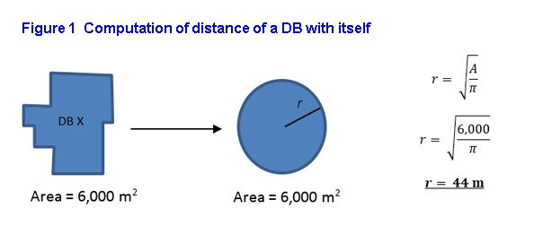
Description for Figure 1
The area of a given DB is linked to a circle of identical area, and the radius of that circle is calculated. The radius of the circle is then assigned as the within distance for that DB. For example, for a DB with an area of 6,000 m2, if the same area were assigned to a circle it would result in a radius of 44 m for that DB.
Measuring presence and size of services
The measure of mass is largely dependent on the nature of the service or amenity that the proximity measure is intended to capture. This section outlines some general considerations and the approaches used for the nine measures developed in this analysis.
In general, two broad approaches could be discerned, uniform weighting and non-uniform weighting. Uniform weighting assigns a value of “1” to each DB that contains an amenity location. The result is that all DBs with a non-zero amount of service are assigned the same mass. It does not assess the potential scale of service provision. In this example, a DB with a corner store would receive the same weight as a DB with a major grocery chain location. Non-uniform weighting utilizes a mass that scales with the size of service, so for example a business’s revenue or the number of employees may be used as a measure of mass.
Generally, weighting by revenue or employment leads to a skewed and dispersed spread of values. As simple intuition would suggest, revenue would differentiate businesses from one another more so than what uniform weighting might achieve. Whether this differentiation of businesses based on revenue creates a good proxy for service provision is arguable, but at a minimum, it makes it possible to differentiate a small grocer from a large supermarket in terms of the amount of services offered. Nonetheless, while raw revenue or employment are imperfect proxies for service availability, e.g., a grocery store with $500,000 in revenue probably does not provide 5 times as much service as a grocery store with a revenue of $100,000, with some elementary transformations to the raw values, a more accurate proxy of service provision can be created.
All BR based masses are derived from a data set of all active businesses from 2017 to 2019 that were extracted from the BR. The information in the BR comes from many sources, of which enterprise-level reporting of activities is one. For most analytical purposes, such a feature is not problematic. In the case of local-level proximity measures, however, enterprise-level reporting may overestimate the mass in areas containing head offices and underestimate it in areas containing operating locations. Take a grocery store chain, for example. The head office may report the number of employees for all its store locations; however, it is the stores that are the point of service locations. To alleviate this issue, a method of redistributing employment from reporting entities to locations was developed. Employment is redistributed proportionally according to the population of the CSD it resides. That is, locations in larger CSDs are presumed to have higher employment than those in smaller CSDs. This issue was avoided with revenue as revenue is typically available at the location level.
Next, entities in the BR with a PO Box as an address were removed because the actual location of the entity could be ascertained, and PO Boxes are likely not the point of service. Further, coordinates of entities may be unreliable at the DB level. While many entities are geocoded at the level of the dissemination block, many are geocoded based on postal codes, and the coordinates may not be accurate to the required precision. Entries in the BR that were not geocoded to the required level of precision were removed. As many of these as possible were re-geocoded by matching addresses to OpenAddresses, a collection of open address data, and then added back into the analysis.
Subsequently, entities that were indicated as self-employed with revenue under $30,000 were removed from the analysis. This was to ensure that the businesses that were analyzed were full-time operations.
The overall employment numbers were benchmarked at the CSD level using the 2016 Census employment by CSD and the 2017-2019 Labour Force Survey (LFS) annual employment values. Because 2016 was the most recent Census year, the 2017-2019 LFS data was used to interpolate the 2016 Census employment data to obtain 2019 values that could be used to benchmark the BR employment data.
Business Register microdata are assigned a 6-digit NAICS category. This allows for considerable flexibility in weighting for all industries or selected industries. The choice of NAICS level for analysis can be expanded or shrunk based on the need of the project (though the quality of results and ability to disseminate them will be impacted the finer the industry level). The specification used resulted from testing alternative options.
Sensitivity to alternative specifications
Throughout the course of implementation, a variety of sensitivity tests were conducted. For each proximity measure, the methodological specifications could be adjusted in many ways. Given the timeframe and resources required to generate these experimental results, a concerted effort was placed on testing methodological elements that were thought to be of most importance. Moreover, most of the testing was implemented for a selected geographic area in the early phase of the project and is only briefly summarized here.
Much of the testing focused on modifying data inputs or values for the mass, distance, and radius variables in the equation. Specifically, testing was done with respect to the following specifications:
- Distance concept – specifically the road network approach (conceptually better) versus the straight-line approach (more practical as it is computationally less onerous).
- Geographical granularity – specifically the DB classification (conceptually better) versus the dissemination areaNote (DA) concept (more practical as it is computationally less taxing).
- Options for mass – specifically using business revenue/employment (in many cases conceptually better) versus uniform weighting business (more practical as it would pose fewer issues related to data confidentiality and suppression).
- Size of radius – specifically large radiuses (in some cases, conceptually required) versus small ones (more practical as it is computationally less taxing).
- Testing options for NAICS categories – specifically, assessing how well the methodology developed performs for different industries and levels of granularity.
To test the road network approach versus geodesic distances, proximity measures were calculated at the DA level for both revenue and employment mass concepts. The mean and median proximity levels were generally higher when computed using a geodesic approach, which makes sense as a geodesic buffer will typically include more DAs in scope than would be present using network distances. Geodesic distances may also lead to certain services being included in the calculation that should not be (for instance, a grocery store on the other side of a river may be close in a geodesic sense, but be far away when constrained to the road network). Because a solution was found to efficiently compute road network distances, that is the concept that was ultimately chosen.
Testing with various specifications suggested that the appropriate mass in the gravity model is likely context-dependent. While revenue may be the appropriate mass when considering certain service types (such as grocery stores), there may be other instances where an equal weighting makes more sense (for example, considering something like access to a gas station or coffee shop, the relative size of that business is likely not of interest).
While it was assumed that the DB would be preferable to the DA for this project, as a smaller geography will better reflect a local measure than a larger geography, testing was done to determine if the difference in results between the two geographic concepts was large. If an analysis using DAs could achieve similar results to DBs with a significantly reduced computational cost, then that would be the proper geography to use. It was found that the measures were not as similar as may have been expected, because while DAs are composed of DBs, in changing the geography from DBs to DAs, the services in range will change (so that a DA, measured from its centroid, does not have access to the same services as the sum of all of its constituent DBs would). Testing conducted with DA-level proximity estimates showed that results were different enough from the DB versions to justify the computational effort and time required to generate the DB-to-DB distances.
Overall, the sensitivity testing suggested that there was a decreasing sensitivity in proximity index given an increase in buffer radius. Testing indicated that the sensitivity of the measure tends to decrease with the increase of the buffer size. This is conceptually straightforward; as the buffer size increases, a typical DB will have access to services in a larger selection of DBs, thus increasing its proximity level. Therefore, the typical proximity index will also increase with buffer size, as the maximum proximity level value is fairly insensitive to changes in buffer size. For instance, testing results indicated that, when using the concept of revenue as a proxy, while increasing the buffer from 1 km to 3 km results in significant changes to the mean index and to average changes in rank, the changes are much smaller for larger buffer values (i.e., increasing the buffer from 10 km to 15 km). This suggests that most choices of buffer size above 10 km are roughly equivalent but that special consideration may have to be given when smaller buffer sizes are to be used.
The aggregations of specific NAICS categories can also have an effect on the proximity measure, especially if specific services are considered to be of particular policy interest. An example is the retail trade category (NAICS 44-45), extracted as a subset of the BR dataset. Certain high-revenue businesses will play a greater role in service provision in the retail trade category than others, and proximity to these high-revenue businesses can be very desirable for residents. However, narrowing down to specific NAICS categories may cause more difficulties related to the confidentiality of data.
Adjustments to meet confidentiality requirements
Confidentiality concerns for this analysis are related specifically to the use of Statistics Canada’s microdata holdings currently protected by provisions of the Statistics Act, specifically the Business Register. The primary confidentiality concern is the risk of being able to identify a specific business’s revenue or number of employees with the proximity measures.
Due to the large volume of data required to calculate the proximity measures, as well as the nature of this data, using standard confidentiality approaches pose several difficulties. There are three main sources that contribute to this confidentiality risk: the geographic classification, the buffer size, and the level of NAICS categories. The lower the level of geographic classification used, the more likely it is to encounter geographies that do not satisfy either the minimum number of businesses and/or encounter problems regarding a dominant business. Likewise, the smaller the buffer size, the more likely it is that some geography will run into issues regarding the minimum number of businesses and dominance. Lastly, stratifying by more detailed NAICS categories increases the likelihood of the aforementioned confidentiality issues.
The most straightforward approach was to classify the confidential input variables (revenue and employment) into intervals. Binning these data combined with the complexity of the computations, reduced the risk of disclosure to the point that the confidentiality requirements were met.
Synopsis of the 10 measures
The methods presented in the previous section were used to compute a set of ten proximity measures. Details on the specifications of each of these measures are presented below.
Proximity to employment measures the closeness of a DB to any DB with a source of employment within a driving distance of 10 km. This measure is derived from the employment counts of all businesses; that is, all North American Industry Classification (NAICS) codes in the Business Register. There were of approximately 3,000,000 businesses used for this measure. By comparison, the total number of Canadian businesses (both with employees and without) for December 2019, according to the Canadian Business CountsNote , is 4,147,129. It should be noted that these numbers are not directly comparable, as three years of data (2017-2019) were used from the BR to construct the proximity measure in addition to the methodological differences in identifying active businesses suitable for analysis between the two.
The employment mass was determined by classifying businesses by the number of employees. Businesses were classified into 8 bins, and those with no employees (self-employed businesses) were removed if their revenue was also less than $30,000. The bins correspond to businesses with 0-4, 5-9, 10-19, 20-49, 50-99, 100-199, 200-499, and 500+ employees. In each case, the mass assigned is the value of the lower bound of its respective bin (for example, a business with 7 employees would be assigned a mass of 5). In the case where the number of employees was reported at the level of a (parent) head office rather than at the level of the individual service locations, the total was split among all children locations using a population weighting. The total employment mass of a dissemination block is the sum of the masses of the services within it.
Proximity to grocery stores measures the closeness of a DB to any DB with a grocery store within a walking distance of 1 km. This measure is derived from the total revenue of all NAICS 4451 (Grocery stores) businesses in the Business Register. There were approximately 11,000 businesses used for this measure. By comparison, the total number of Canadian businesses under this NAICS code (both with employees and without) for December 2019, according to the Canadian Business Counts, is 22,579. The total mass of a dissemination block is the sum of the masses of the services within it.
The mass for each business was determined from its revenue by assigning a value of 1, 2, 3, or 4, depending on what revenue quartile the business belonged to at the national level. This sort of weighting ensures that there is at most a fourfold increase in mass when comparing a small grocery provider with a large grocery provider, whereas using revenue directly may lead to a difference of multiple orders of magnitude from the smallest mass to the largest. In the case where the number of employees was reported at the level of a (parent) head office rather than at the level of the individual service locations, the total was split among all children locations using a population weighting.
Proximity to pharmacies measures the closeness of a DB to any DB with a pharmacy or a drug store within a walking distance of 1 km. This measure is derived from the presence of all NAICS 446110 (Pharmacies and drug stores) businesses in the Business Register. There were approximately 27,000 businesses used for this measure. By comparison, the total number of Canadian businesses under this NAICS code (both with employees and without) for December 2019, according to the Canadian Business Counts, is 12,965. The large number of businesses used in the proximity measure calculation relative to the count of businesses in the Canadian Business Counts may indicate that pharmacies are more significantly impacted by the methodological differences, such as using 3 years of data (2017 to 2019) than the other business types considered.
Because the fundamental service provided by a pharmacy is not expected to scale with revenue or number of employees, a uniform mass was chosen. This also avoids potential issues where pharmacies and drug stores may have non-pharmaceutical sources of revenue (groceries, etc.) which may obfuscate the “actual” level of service provision. As the mass is uniform, the mass of a dissemination block is 1 if at least one service resides within it.
Proximity to health care measures the closeness of a DB to any DB with a health care facility within a driving distance of 3 km. This measure is derived from the employment counts of all NAICS 6211 (Offices of physicians), 6212 (Offices of dentists), 6213 (Offices of other health practitioners), 621494 (Community health centres), and 622 (Hospitals) businesses in the Business Register. There were approximately 180,000 businesses used for this measure. By comparison, the total number of Canadian businesses under these NAICS codes (both with employees and without) for December 2019, according to the Canadian Business Counts, is 189,426.
The employment mass was determined by classifying businesses by the number of employees. Businesses were classified into 8 bins, and those with no employees (self-employed businesses) were removed if their revenue was also less than $30,000. The bins correspond to businesses with 0-4, 5-9, 10-19, 20-49, 50-99, 100-199, 200-499, and 500+ employees. The total mass of a dissemination block is the sum of the masses of the services within it.
Proximity to child care measures the closeness of a DB to any DB with a child care facility within a walking distance of 1.5 km. This measure is derived from the presence of all NAICS 624410 (Child day-care services) businesses in the Business Register, except for self-employed businesses with revenue less than $30,000 a year. There were approximately 39,000 businesses used for this measure. By comparison, the total number of Canadian businesses under these NAICS codes (both with employees and without) for December 2019, according to the Canadian Business Counts, is 41,383.
Because this service includes a relatively large proportion of self-employed businesses that were found to complicate an employment-based mass, a uniform mass was chosen. As the mass is uniform, the mass of a DB is 1 if at least one service resides within it (so that all DBs that contain a non-zero amount of service are assigned the same mass).
Proximity to primary education measures the closeness of a DB to any DB with a primary school within a walking distance of 1.5 km. Primary schools are classified as education facilities with an International Standard Classification of Education (ISCED) level of 1. The data source is a conglomeration of the Open Database of Education FacilitiesNote and other sources of education facilities. In total, approximately 11,000 primary schools were included for this measure. As the mass is uniform, the mass of a DB is 1 if at least one service resides within it (so that all DBs that contain a non-zero amount of service are assigned the same mass).
The ODEF contains schools categorized by the ISCED levels, which are levels associated with grade ranges. Details on the correspondence are provided in Statistics Canada (2019), for the purpose of these measure the following ISCED are used: Elementary (ISCED1), which correspond to grade 1-6; Junior secondary (ISCED2) and Senior secondary (ISCED3) corresponding to grades 7-9 and 10-12, respectively. The advantage of the ODEF over the BR in this respect is that elementary schools and high schools may be considered separately. When the total number of schools in these categories available in both databases is considered, it is evident that the ODEF is preferable to the BR. The BR contains approximately 3,300 schools in the Elementary and Secondary schools category. By contrast, the ODEF contains over 16,000 entries categorized as one of either ISCED1, ISCED2, or ISCED3.
The educational facilities data was geocoded when necessary and filtered to exclude non-public schools whenever possible. It was occasionally necessary to impute the ISCED level from a grade range when possible, and if not, then to infer it from the name of the school.
Proximity to secondary education measures the closeness of a DB to any DB with a secondary school within a walking distance of 1.5 km. The data source is a conglomeration of the Open Database of Education Facilities and other sources of education facilities where secondary schools are classified as ISCED2 and/or ISCED3 (corresponding to grades 7-9 and 10-12, respectively).
In total, approximately 5,000 secondary schools were included for this measure. As the mass is uniform, the mass of a DB is 1 if at least one service resides within it (so that all DBs that contain a non-zero amount of service are assigned the same mass).
Proximity to public transit measures the closeness of a DB to any source of public transportation within a 1 km walking distance. This measure of mass is derived from the number of all trips between 7:00 a.m. - 10:00 a.m. from a conglomeration of General Transit Feed Specification (GTFS) data sources.
Proximity to public transit is computed using GTFS data. The proximity measure presented in this analysis uses the number of individual buses or trains that serve a stop in a given timeframe (between 7 a.m. and 10 a.m. on a weekday morning). For this measure, the mass is not applied to the dissemination block, but to the individual transit stops.
While there is no list of all transit systems in Canada, let alone a list of all transit systems in Canada with GTFS data available, effort has been made to collect as many as possible. This resulted in a collection of 94 individual GTFS feeds that have been used in the construction of the database, which includes both local transit systems and inter-municipal transit systems. Not all data sources frequently update their posted GTFS data, and so the reference periods of the datasets are not uniform. To create a measure reflecting average weekday morning service, for all datasets the number of trips on a Wednesday morning was determined. There are approximately 130,000 individual transit stops used for this measure.
For this measure, an attempt was made to identify regions that have public transit but that do not have GTFS data available, or that seem to have GTFS data available (inferred from the integration of the transit system’s schedule with Google Maps). When the existence of transit data was inferred, and it could not be found through web searches, municipalities and transit authorities were contacted to request the data. The proximity measures database indicates whether transit data exists in the transit_na column, where entries have been assigned to code 2 if the GTFS data was not available but was inferred to exist for that CSD. Note that this in an imperfect mapping, as there is not a relationship between CSD boundaries and transit systemsNote .
Proximity to neighbourhood parks measures the closeness of a DB to any DB with a neighbourhood park within a 1 km walking distance. This measure is derived from the presence of all parks from a conglomeration of authoritative open data sources and OpenStreetMap. In total, approximately 48,000 parks were used for this measure. As the mass is uniform, the mass of a DB is 1 if at least one service resides within it (so that all DBs that contain a non-zero amount of service are assigned the same mass).
After collecting parks data from open data portals, a small number of records were geocoded, and all the records were cleaned using the park type information when it was available. There is no standard classification system for parks, and so datasets also occasionally included entries that were considered to be outside of scope (for example, museums, golf courses, and arenas). A number of the parks were filtered out when the type was considered out of scope.
For the OpenStreetMap data, not all parks contained names. When they did contain names, and those names contained the words “provincial”, “national”, or “regional”, they were removed. This was to ensure that as much as possible only local community parks were included. Because there were likely to be duplicate parks between the OpenStreetMap data and what was collected from open data sources, the full park dataset was deduplicated based on proximity. A threshold of 25 metres was selected, so that two parks within 25 metres of each other were considered duplicates and one was removed. This threshold was chosen after performing a nearest-neighbour analysis to determine the mean shortest distance between parks in the dataset, and was chosen to be significantly smaller than the mean distance. Conceptually, it was also chosen to be relatively short as it is possible for parks to be fairly near to each other (for instance, on either side of a street), and so a short distance was deemed appropriate.
Proximity to libraries measures the closeness of a DB to any DB with a library within a 1.5 km walking distance. This measure is derived from the presence of all libraries from a conglomeration of open and public data sources. In total, approximately 3,000 libraries were used for this measure. As the mass is uniform, the mass of a DB is 1 if at least one service resides within it (so that all DBs that contain a non-zero amount of service are assigned the same mass).
The library data, when necessary, were geocoded with a combination of Nominatim, Bing, and manually through Internet searches. Entries that could not be geocoded accurately were dropped. Libraries where the names suggested they were university libraries, or private professional libraries, were also excluded from the current specification. Finally, libraries were de-duplicated by proximity. A threshold of 150 metres was used so that two libraries within 150 metres of each other were considered duplicates and one was removed. This threshold was chosen during processing after performing a nearest-neighbour analysis to determine the mean distance between libraries, and was chosen to be significantly smaller than the mean shortest distance between them. Conceptually, this distance can correspond to the scale of a standard city block, and it is considered unlikely to have two public libraries within one or two blocks from each other.
Results
This section presents the results for the specifications detailed in the previous section, starting from the most general measure of proximity to employment, followed by measures generated with business register data, and then by the remaining three measures entirely based on open and publicly available data.
For each measure, results are presented in terms of the share of population falling into different ranges of proximity to that service or amenity. Results are tabulated by Census Metropolitan Area (CMA), Census Agglomerations (CA) (thereafter referred jointly as urbanized areas) and for areas outside CMA/CA, referred as rural.Note
Within each regional type, the tables present the percentage of population falling into three different range of the proximity measures. For simplicity and comparability, three groups are defined as Bottom, Middle, and Top. These fields indicate the percentage of population falling into three categories corresponding to the distribution of the proximity index values (ranging from 0 to 1) by terciles. The field defined as Outside represents the percentage of population living in DB outside the radius used in the computation of the specific service or amenity; that is, the population with no access to that service or amenity, given the specifications that are currently used.
In addition, column “F” of each table reports the percentage of population living in DBs for which the proximity measure results are “too unreliable to be published.” These columns are identical for all of the following tables because when the results are unreliable, all proximity measures for the DB are suppressed. In relation to this product, the symbol indicates that a proximity index value was suppressed due inconsistency between data sources and/or very small population counts. These values are reported in all tables for completeness, so that regional percentages add up to 100% in each province.
Each table presents the results by Province/Territory and the total for Canada (this is based on the aggregation of all DBs). In addition, the last row of the table shows the regional percentage relative to the total population of Canada (instead of the total population of that type of region).
It should be noted that the full Proximity Measures Database was released in CSV format.Note For each DB record, the database includes the unique DB identifier code, population counts and the ten normalized index values and a composite measure of amenity dense neighbourhood. In addition, the results for each dissemination block can be visualized using an online mapping application, which was first developed for quality checks and validation, and then further developed and released as the Proximity Measures Data Viewer.Note The Viewer allows users to switch between views of different measures, search areas by Census Subdivision (municipality) and zoom quickly to different localities. Both the database and data viewer allow for granular analysis, comparison and benchmarking or neighbourhood and localities across Canada.
Proximity to employment
Proximity to employment provides a broad understanding of the geographic concentration of employment, using the most comprehensive and granular database with some information on business employment (i.e., the Business Register), as well as most granular standard administrative geography of Canada. Hence, the results are driven by the concentration of employment in urban areas, as well as by the size of urban agglomeration.
Most Canadians (over 98%) live within 10 km drive from businesses providing employment. As one would expect, the distribution changes considerably between more urbanized areas, where virtually all the population has some degree of proximity (10 km driving distance) to employment, and rural regions, where 8.4% of the population live beyond the 10 km driving mark for employer businesses (Table 3).
Table 3 Proximity to employment: percentage of population, by province and territories, presents results by provinces and territory and highlights the main differences between Newfoundland and Labrador, Prairies provinces and Territories, on the one hand, and the other provinces of Canada, on the other hand. The first group, with more disperse rural population, reports between about 12% and 40% of that population leaving beyond a 10 km from a business with employment. The second group has generally marginal percentages (less than 4%) of rural population living outside the 10 km reach from a business with employment.
This measure depicts a broad picture of spatial concentration of any type of employment generated by business with employees, and the measure could be recomputed for specific types of employment and could be further enhanced to account for labour supply factors in the same proximity ranges. Also, it should be noted that this proximity measure is computed using employment estimates included in the 2019 vintage of the BR. Following the COVID-19 crisis, this measure assumes particular relevance for benchmarking of potential spatial changes in employment location as well as for the identification of neighbourhoods that may be more severely affected by these adjustments in the labour market.
| Geography | CMA | CA | Rural | ||||||||||||
|---|---|---|---|---|---|---|---|---|---|---|---|---|---|---|---|
| Outside | Bottom | Middle | Top | Note F: too unreliable to be published | Outside | Bottom | Middle | Top | Note F: too unreliable to be published | Outside | Bottom | Middle | Top | Note F: too unreliable to be published | |
| NL | Note ..: not available for a specific reference period | 7.8 | 51.7 | 40.5 | 0.0 | 0.2 | 21.9 | 77.0 | 0.2 | 0.7 | 11.9 | 61.5 | 22.6 | 0.1 | 4.0 |
| PE | Note ..: not available for a specific reference period | Note ..: not available for a specific reference period | Note ..: not available for a specific reference period | Note ..: not available for a specific reference period | Note ..: not available for a specific reference period | .. | 24.0 | 63.0 | 13.1 | 0.0 | 0.0 | 87.0 | 12.3 | Note ..: not available for a specific reference period | 0.6 |
| NS | 0.0 | 22.6 | 35.8 | 41.3 | 0.1 | 0.2 | 31.3 | 66.5 | 1.9 | 0.1 | 0.5 | 67.6 | 31.7 | 0.0 | 0.2 |
| NB | 0.1 | 22.4 | 50.4 | 26.9 | 0.2 | 0.2 | 36.9 | 56.3 | 6.5 | 0.1 | 0.5 | 73.7 | 25.7 | Note ..: not available for a specific reference period | 0.1 |
| QC | 0.0 | 4.4 | 24.8 | 70.8 | 0.0 | 0.1 | 15.7 | 63.7 | 20.4 | 0.1 | 0.9 | 54.1 | 44.4 | 0.1 | 0.5 |
| ON | 0.0 | 4.6 | 20.8 | 74.6 | 0.0 | 0.0 | 22.7 | 62.2 | 14.9 | 0.2 | 2.2 | 55.3 | 41.5 | 0.2 | 0.8 |
| MB | 0.2 | 6.3 | 19.3 | 74.1 | 0.1 | 1.6 | 11.7 | 68.4 | 17.9 | 0.5 | 21.5 | 38.6 | 33.0 | 0.1 | 6.8 |
| SK | 1.6 | 5.1 | 21.2 | 71.8 | 0.2 | 4.5 | 9.9 | 75.0 | 9.4 | 1.1 | 39.6 | 27.7 | 23.1 | 0.0 | 9.5 |
| AB | 0.1 | 6.0 | 29.6 | 64.2 | 0.1 | 0.8 | 6.9 | 58.8 | 33.2 | 0.4 | 19.9 | 37.9 | 39.0 | 0.2 | 3.0 |
| BC | 0.0 | 3.0 | 18.7 | 78.3 | 0.0 | 0.1 | 16.0 | 66.5 | 17.3 | 0.1 | 3.2 | 51.9 | 44.2 | 0.1 | 0.7 |
| YT | Note ..: not available for a specific reference period | Note ..: not available for a specific reference period | Note ..: not available for a specific reference period | Note ..: not available for a specific reference period | Note ..: not available for a specific reference period | 7.5 | 20.1 | 65.9 | 6.4 | 0.0 | 38.3 | 34.2 | 10.2 | Note ..: not available for a specific reference period | 17.3 |
| NT | Note ..: not available for a specific reference period | Note ..: not available for a specific reference period | Note ..: not available for a specific reference period | Note ..: not available for a specific reference period | Note ..: not available for a specific reference period | 0.0 | 11.5 | 81.4 | 7.0 | 0.1 | 22.5 | 27.7 | 28.6 | Note ..: not available for a specific reference period | 21.1 |
| NU | Note ..: not available for a specific reference period | Note ..: not available for a specific reference period | Note ..: not available for a specific reference period | Note ..: not available for a specific reference period | Note ..: not available for a specific reference period | Note ..: not available for a specific reference period | Note ..: not available for a specific reference period | Note ..: not available for a specific reference period | Note ..: not available for a specific reference period | Note ..: not available for a specific reference period | 39.3 | 6.8 | 28.1 | 0.5 | 25.4 |
| Canada | 0.1 | 5.1 | 23.2 | 71.6 | 0.1 | 0.4 | 18.2 | 64.0 | 17.1 | 0.2 | 8.4 | 51.3 | 37.9 | 0.1 | 2.2 |
| % of total population | 0.0 | 3.6 | 16.5 | 50.8 | 0.0 | 0.1 | 2.2 | 7.8 | 2.1 | 0.0 | 1.4 | 8.6 | 6.4 | 0.0 | 0.4 |
|
Note: Proximity to employment measures the closeness of a dissemination block to any dissemination block with a source of employment, as captured by the location of businesses with employees (all NAICS codes), within a driving network distance of 10 km is used for the computation. Source: Authors’ computation. |
|||||||||||||||
Proximity to grocery stores
For most Canadians, a visit to a grocery store to buy food is a daily necessity, for this reason proximity was specified as having this type of store within 1 km walking distance. Across Canada nearly half (46%) of the population live in a neighbourhood or locality with this characteristic. However, there are major differences between urbanized and rural areas as well as among provinces and territories (Table 4).
Overall, the majority (55%) of population living in the CMAs have some degree of proximity to a grocery store; this percentage drops to 30% for those living in CAs and to 16% for those living in rural area (Table 4), with Quebec, Ontario, Manitoba, and British Columbia reporting the largest shares of metropolitan population with proximity to large volume of grocery service. On the contrary, the Atlantic Provinces presents the highest share of CMA, as well as CA, population outside the proximity radius of 1 km from grocery stores (above 64% or 74%, respectively). The Proximity Measures Data Viewer provides a mapping of these neighbourhoods across Canada.
For metropolitan areas this proximity measure can contribute to the understanding of so-called food deserts, areas that provide limited or no access to food retails within short walking distance. Nevertheless, it should be kept in mind that the current specification accounts for only one type of businesses (NAICS code) that provides access to food. Although grocery stores are the most common type of food retail accessed by Canadian families, several other types of food retails provide various degrees of access to food (e.g., farmers markets, etc.).
In rural areas, it is not surprising that access to grocery requires travelling more than 1 km for the vast majority of people. However, among the services considered in this analysis, grocery remains one of the most accessible to the rural population as well. In all the provinces, between about 10% and 20% of the rural population live within a 1 km walk from a grocery store, which is likely to be the main type of stores to be found in rural and small-town Canada.
| Geography | CMA | CA | Rural | ||||||||||||
|---|---|---|---|---|---|---|---|---|---|---|---|---|---|---|---|
| Outside | Bottom | Middle | Top | Note F: too unreliable to be published | Outside | Bottom | Middle | Top | Note F: too unreliable to be published | Outside | Bottom | Middle | Top | Note F: too unreliable to be published | |
| NL | 70.0 | 10.2 | 12.8 | 6.9 | 0.0 | 82.8 | 5.7 | 6.7 | 4.2 | 0.7 | 85.1 | 5.5 | 3.9 | 1.6 | 4.0 |
| PE | Note ..: not available for a specific reference period | Note ..: not available for a specific reference period | Note ..: not available for a specific reference period | Note ..: not available for a specific reference period | Note ..: not available for a specific reference period | 74.0 | 9.4 | 9.3 | 7.3 | 0.0 | 89.8 | 3.6 | 4.4 | 1.6 | 0.6 |
| NS | 64.3 | 13.6 | 11.1 | 10.8 | 0.1 | 81.3 | 7.0 | 8.0 | 3.5 | 0.1 | 89.8 | 4.1 | 4.7 | 1.2 | 0.2 |
| NB | 77.9 | 7.5 | 8.1 | 6.2 | 0.2 | 84.9 | 4.9 | 6.4 | 3.6 | 0.1 | 88.5 | 5.6 | 4.2 | 1.6 | 0.1 |
| QC | 41.8 | 15.7 | 15.3 | 27.3 | 0.0 | 62.4 | 12.8 | 14.3 | 10.3 | 0.1 | 79.4 | 8.2 | 7.6 | 4.4 | 0.5 |
| ON | 44.3 | 18.3 | 16.7 | 20.6 | 0.0 | 70.5 | 11.9 | 11.0 | 6.3 | 0.2 | 83.8 | 5.9 | 6.5 | 3.0 | 0.8 |
| MB | 43.2 | 16.4 | 19.1 | 21.2 | 0.1 | 65.7 | 12.6 | 11.3 | 9.8 | 0.5 | 78.8 | 5.2 | 5.2 | 3.9 | 6.8 |
| SK | 52.4 | 18.4 | 17.0 | 11.9 | 0.2 | 65.7 | 15.0 | 12.2 | 6.0 | 1.1 | 72.3 | 5.6 | 8.1 | 4.6 | 9.5 |
| AB | 52.0 | 19.1 | 16.4 | 12.4 | 0.1 | 62.3 | 16.4 | 13.2 | 7.7 | 0.4 | 79.8 | 6.6 | 6.9 | 3.7 | 3.0 |
| BC | 36.8 | 17.6 | 15.0 | 30.6 | 0.0 | 73.5 | 10.0 | 9.8 | 6.6 | 0.1 | 83.9 | 6.3 | 5.9 | 3.2 | 0.7 |
| YT | Note ..: not available for a specific reference period | Note ..: not available for a specific reference period | Note ..: not available for a specific reference period | Note ..: not available for a specific reference period | Note ..: not available for a specific reference period | 72.6 | 11.0 | 12.7 | 3.6 | 0.0 | 81.4 | 1.3 | Note ..: not available for a specific reference period | Note ..: not available for a specific reference period | 17.3 |
| NT | Note ..: not available for a specific reference period | Note ..: not available for a specific reference period | Note ..: not available for a specific reference period | Note ..: not available for a specific reference period | Note ..: not available for a specific reference period | 63.5 | 13.0 | 16.0 | 7.4 | 0.1 | 57.1 | 5.7 | 10.1 | 6.0 | 21.1 |
| NU | Note ..: not available for a specific reference period | Note ..: not available for a specific reference period | Note ..: not available for a specific reference period | Note ..: not available for a specific reference period | Note ..: not available for a specific reference period | Note ..: not available for a specific reference period | Note ..: not available for a specific reference period | Note ..: not available for a specific reference period | Note ..: not available for a specific reference period | Note ..: not available for a specific reference period | 59.6 | 4.3 | 6.1 | 4.6 | 25.4 |
| Canada | 44.7 | 17.4 | 16.0 | 21.9 | 0.1 | 69.6 | 11.7 | 11.3 | 7.1 | 0.2 | 81.5 | 6.4 | 6.5 | 3.4 | 2.2 |
| % of total population | 31.7 | 12.3 | 11.4 | 15.5 | 0.0 | 8.5 | 1.4 | 1.4 | 0.9 | 0.0 | 13.7 | 1.1 | 1.1 | 0.6 | 0.4 |
|
Note: Proximity to grocery stores measures the closeness of a dissemination block to any dissemination block with a grocery store and within a walking network distance of 1 km. Grocery stores are businesses classified as NAICS 4451 (Grocery stores) in the Business Register. Source: Authors’ computation. |
|||||||||||||||
Proximity to pharmacies
Access to pharmacies and drug stores is generally perceived as a basic necessity in the daily life of a typical family. For this reason, proximity is measured as the presence of this service within a 1 km walking distance; there is no weight attributed to the point of service, so the measure is entirely driven by physical distance to the service.
With this specification, nearly 60% of Canadians live in proximity to pharmacy and drug stores (Table 5). The largest proportion of the population living in proximity to these services is in larger urban areas (CMAs). In fact, in these areas slightly over 70% of the population live within 1 km walking distance to a pharmacy. Ontario and British Columbia present the highest share of large urban populations living in proximity as well as the highest level of proximity access (top tercile of the proximity measure distribution). All the other provinces with the exceptions of the Atlantic Provinces have a majority of CMA population living in proximity to these services.
Proximity to this type of service (1 km walking distance) is enjoyed by a sizable lower share of the population of smaller metro areas (CA) and an even smaller share of the population in the rural areas. But there are still large differences between provinces. Overall, close to one half of the CA population in the Prairies is located within 1 km walking distance to a pharmacy. In the Atlantic Provinces, this share drops to about 30%. In the Territories, the lowest proximity to pharmacy and drug stores is for the CAs residents of the Yukon. By contrast, the residents living in the CAs of the Northwest Territories have relatively good access to drug stores.
About 20% of residents in rural areas in Canada live in proximity to a pharmacy (walking distance of 1 km). Overall, residents of rural areas from Ontario, Quebec and British Columbia are more likely to live in proximity to this type of service. While rural population in the Atlantic Provinces are the least likely to live in proximity to these services.
| Geography | CMA | CA | Rural | ||||||||||||
|---|---|---|---|---|---|---|---|---|---|---|---|---|---|---|---|
| Outside | Bottom | Middle | Top | Note F: too unreliable to be published | Outside | Bottom | Middle | Top | Note F: too unreliable to be published | Outside | Bottom | Middle | Top | Note F: too unreliable to be published | |
| NL | 57.7 | 17.2 | 15.0 | 10.1 | 0.0 | 69.5 | 16.4 | 10.4 | 3.1 | 0.7 | 86.7 | 6.3 | 2.6 | 0.4 | 4.0 |
| PE | .. | Note ..: not available for a specific reference period | Note ..: not available for a specific reference period | Note ..: not available for a specific reference period | Note ..: not available for a specific reference period | 67.1 | 12.0 | 9.7 | 11.2 | 0.0 | 89.5 | 6.4 | 3.3 | 0.2 | 0.6 |
| NS | 50.2 | 19.9 | 14.2 | 15.6 | 0.1 | 70.7 | 13.4 | 10.6 | 5.2 | 0.1 | 84.9 | 7.9 | 4.7 | 2.3 | 0.2 |
| NB | 63.9 | 15.6 | 12.3 | 8.0 | 0.2 | 69.6 | 15.6 | 8.5 | 6.1 | 0.1 | 86.2 | 8.0 | 4.2 | 1.5 | 0.1 |
| QC | 32.7 | 19.1 | 20.1 | 28.1 | 0.0 | 56.2 | 17.0 | 14.2 | 12.4 | 0.1 | 79.9 | 9.5 | 6.9 | 3.1 | 0.5 |
| ON | 23.6 | 20.7 | 25.1 | 30.6 | 0.0 | 57.6 | 17.8 | 13.7 | 10.7 | 0.2 | 79.2 | 9.6 | 7.1 | 3.3 | 0.8 |
| MB | 28.9 | 21.6 | 27.3 | 22.1 | 0.1 | 50.0 | 18.6 | 15.3 | 15.6 | 0.5 | 77.6 | 7.7 | 5.5 | 2.3 | 6.8 |
| SK | 34.3 | 24.4 | 25.4 | 15.7 | 0.2 | 52.2 | 15.0 | 18.4 | 13.3 | 1.1 | 79.3 | 5.8 | 3.5 | 1.9 | 9.5 |
| AB | 32.5 | 25.3 | 25.2 | 16.8 | 0.1 | 43.9 | 26.7 | 18.0 | 11.0 | 0.4 | 77.0 | 10.0 | 6.8 | 3.2 | 3.0 |
| BC | 24.1 | 19.2 | 21.1 | 35.6 | 0.0 | 61.3 | 15.3 | 13.5 | 9.8 | 0.1 | 79.9 | 10.6 | 5.7 | 3.1 | 0.7 |
| YT | Note ..: not available for a specific reference period | Note ..: not available for a specific reference period | Note ..: not available for a specific reference period | Note ..: not available for a specific reference period | Note ..: not available for a specific reference period | 91.7 | 1.4 | 1.8 | 5.0 | 0.0 | 82.7 | Note ..: not available for a specific reference period | Note ..: not available for a specific reference period | Note ..: not available for a specific reference period | 17.3 |
| NT | Note ..: not available for a specific reference period | Note ..: not available for a specific reference period | Note ..: not available for a specific reference period | Note ..: not available for a specific reference period | Note ..: not available for a specific reference period | 64.0 | 16.2 | 8.2 | 11.4 | 0.1 | 71.6 | 6.0 | 1.3 | Note ..: not available for a specific reference period | 21.1 |
| NU | Note ..: not available for a specific reference period | Note ..: not available for a specific reference period | Note ..: not available for a specific reference period | Note ..: not available for a specific reference period | Note ..: not available for a specific reference period | Note ..: not available for a specific reference period | Note ..: not available for a specific reference period | Note ..: not available for a specific reference period | Note ..: not available for a specific reference period | Note ..: not available for a specific reference period | 70.1 | 2.6 | 1.8 | 0.0 | 25.4 |
| Canada | 28.3 | 20.7 | 23.1 | 27.8 | 0.1 | 57.9 | 17.5 | 13.9 | 10.5 | 0.2 | 80.0 | 9.0 | 6.0 | 2.8 | 2.2 |
| % of total population | 20.1 | 14.7 | 16.4 | 19.8 | 0.0 | 7.1 | 2.1 | 1.7 | 1.3 | 0.0 | 13.5 | 1.5 | 1.0 | 0.5 | 0.4 |
|
Note: Proximity to pharmacies measures the closeness of a DB to any DB with a pharmacy or a drug store within a walking distance of 1 km. This measure is derived from the presence of all NAICS 446110 (Pharmacies and drug stores) businesses in the Business Register. Source: Authors’ computation. |
|||||||||||||||
Proximity to health care
Measure of proximity to health care facilities have acquired an even greater relevance in the last year, which has led to more data development on the geolocation of health care facilities.Note This measure is based on the location of selected types of health care facilities from Business Register data (see section 3).
Overall, the results indicate that about 88% of the Canadian population live in a neighbourhood or locality that is within 3 km drive from a health care facility (Table 6). Canadians living in larger metropolitan areas are in vast majority (97%) living within a 3 km drive from a health care facility. For resident of smaller metro areas, this percentage drops to 87%; while in aggregate terms, only about half of rural residents enjoy the same degree of proximity to this type of facility.
Residents of British Columbia living in CMAs enjoy the highest degree of proximity to this service, as measured by both distance and volume of service, with less than 1% of residents living in neighbourhoods more than 3 km driving distance from this service and nearly 56% of the population falling in the top tercile of the proximity measure distribution. This province is followed by Ontario (less than 3% outside and 45.6% living in the top tercile) and Quebec (less than 3% outside and 43.8% in the top tercile).
Results for smaller urban areas (CA) point to some macro-regional diversity, with residents living in CAs of Atlantic Provinces slightly more likely to live outside the 3 km driving distance from a health care facility. Finally, about 50% of residents living in rural areas need to drive more than 3 km to access health care services. The lowest proportion of population living in rural areas and needing to drive more for accessing health care services is British Columbia (37.7%), while the highest shares are found in Prince Edward Island (74.1%), Saskatchewan (69.4%) and Newfoundland and Labrador (62.9%).
| Geography | CMA | CA | Rural | ||||||||||||
|---|---|---|---|---|---|---|---|---|---|---|---|---|---|---|---|
| Outside | Bottom | Middle | Top | Note F: too unreliable to be published | Outside | Bottom | Middle | Top | Note F: too unreliable to be published | Outside | Bottom | Middle | Top | Note F: too unreliable to be published | |
| NL | 3.0 | 43.3 | 31.1 | 22.6 | 0.0 | 15.8 | 43.9 | 27.6 | 12.0 | 0.7 | 62.9 | 22.3 | 7.7 | 3.2 | 4.0 |
| PE | Note ..: not available for a specific reference period | Note ..: not available for a specific reference period | Note ..: not available for a specific reference period | Note ..: not available for a specific reference period | Note ..: not available for a specific reference period | 18.9 | 37.6 | 29.4 | 14.1 | 0.0 | 74.1 | 19.8 | 5.3 | 0.2 | 0.6 |
| NS | 7.5 | 38.0 | 31.1 | 23.2 | 0.1 | 24.0 | 40.2 | 17.8 | 17.9 | 0.1 | 51.6 | 31.9 | 12.5 | 3.9 | 0.2 |
| NB | 15.9 | 33.7 | 28.3 | 21.9 | 0.2 | 21.5 | 46.9 | 23.5 | 8.0 | 0.1 | 55.9 | 35.8 | 6.8 | 1.4 | 0.1 |
| QC | 2.3 | 19.3 | 34.5 | 43.8 | 0.0 | 9.4 | 34.4 | 33.2 | 22.9 | 0.1 | 43.5 | 42.8 | 11.6 | 1.6 | 0.5 |
| ON | 2.4 | 14.1 | 37.9 | 45.6 | 0.0 | 16.2 | 26.0 | 26.5 | 31.2 | 0.2 | 47.4 | 28.3 | 14.6 | 8.9 | 0.8 |
| MB | 4.6 | 15.7 | 42.1 | 37.5 | 0.1 | 12.2 | 16.0 | 39.3 | 32.1 | 0.5 | 59.8 | 16.5 | 12.8 | 4.1 | 6.8 |
| SK | 7.0 | 19.6 | 40.1 | 33.0 | 0.2 | 10.8 | 19.6 | 42.6 | 25.9 | 1.1 | 69.4 | 11.2 | 7.8 | 2.2 | 9.5 |
| AB | 3.7 | 17.2 | 47.3 | 31.8 | 0.1 | 3.9 | 20.7 | 54.1 | 20.9 | 0.4 | 56.3 | 21.9 | 17.1 | 1.7 | 3.0 |
| BC | 0.8 | 13.9 | 29.4 | 55.9 | 0.0 | 8.4 | 36.5 | 31.9 | 23.1 | 0.1 | 37.7 | 41.2 | 18.2 | 2.2 | 0.7 |
| YT | Note ..: not available for a specific reference period | Note ..: not available for a specific reference period | Note ..: not available for a specific reference period | Note ..: not available for a specific reference period | Note ..: not available for a specific reference period | 15.2 | 57.2 | 7.3 | 20.2 | 0.0 | 59.9 | 22.3 | 0.5 | Note ..: not available for a specific reference period | 17.3 |
| NT | Note ..: not available for a specific reference period | Note ..: not available for a specific reference period | Note ..: not available for a specific reference period | Note ..: not available for a specific reference period | Note ..: not available for a specific reference period | 2.5 | 39.1 | 53.3 | 4.8 | 0.1 | 42.0 | 32.3 | 4.7 | Note ..: not available for a specific reference period | 21.1 |
| NU | Note ..: not available for a specific reference period | Note ..: not available for a specific reference period | Note ..: not available for a specific reference period | Note ..: not available for a specific reference period | Note ..: not available for a specific reference period | Note ..: not available for a specific reference period | Note ..: not available for a specific reference period | Note ..: not available for a specific reference period | Note ..: not available for a specific reference period | Note ..: not available for a specific reference period | 46.2 | 13.2 | 13.7 | 1.4 | 25.4 |
| Canada | 2.7 | 16.7 | 37.0 | 43.6 | 0.1 | 12.0 | 31.1 | 32.8 | 23.9 | 0.2 | 50.3 | 30.7 | 13.0 | 3.7 | 2.2 |
| % of total population | 1.9 | 11.8 | 26.2 | 30.9 | 0.0 | 1.5 | 3.8 | 4.0 | 2.9 | 0.0 | 8.5 | 5.2 | 2.2 | 0.6 | 0.4 |
|
Note: Proximity to health care measures the closeness of a DB to any DB with a health care facility within a driving distance of 3 km. This measure is derived from the employment counts of all NAICS 6211 (Offices of physicians), 6212 (Offices of dentists), 6213 (Offices of other health practitioners), 621494 (Community health centres), and 622 (Hospitals) businesses in the Business Register. Source: Authors’ computation. |
|||||||||||||||
Proximity to primary education
Overall, about 70% of Canadians live within 1.5 km walking distance from a primary education facility (Table 7). Primary education comprises schools teaching grade 1 to grade 6. The presence and proximity to a primary school in a neighbourhood is a major determinant of location choice for families with children; hence, proximity to these facilities is likely a major determinant in the quality of life for children and parents alike.
The percentage of people living in neighbourhoods in proximity to primary education is higher in CMAs, where over 80% of residents live in neighbourhoods that are in proximity to a primary education facility (Table 7). Nevertheless, residents of CMAs in the Atlantic Provinces are more likely to live outside the 1.5 km walking distance from these facilities, with New Brunswick and Newfoundland and Labrador reporting about 50% of their CMA population living outside this boundary (Table 7). On the contrary, residents of CMAs in Manitoba, Saskatchewan and British Columbia are those more likely to live in proximity to primary education facilities (75% or more).
Generally, less than 30% of rural residents, which include villages and small towns, are located in a 1.5 km walking distance from educational facilities. When the share of population outside this distance boundary is combined with the share of population living in dissemination block for which there is no reliable information (column F) the results are similar for rural regions across all provinces. Nevertheless, Atlantic Provinces are once again those with higher percentage of population living beyond the 1.5 km walking distance from schools, with Prince Edward Island reporting 87% and Nova Scotia and New Brunswick almost 80% of their rural population.
| Geography | CMA | CA | Rural | ||||||||||||
|---|---|---|---|---|---|---|---|---|---|---|---|---|---|---|---|
| Outside | Bottom | Middle | Top | Note F: too unreliable to be published | Outside | Bottom | Middle | Top | Note F: too unreliable to be published | Outside | Bottom | Middle | Top | Note F: too unreliable to be published | |
| NL | 50.1 | 19.6 | 20.2 | 10.0 | 0.0 | 64.5 | 19.0 | 11.7 | 4.1 | 0.7 | 73.5 | 15.1 | 5.9 | 1.5 | 4.0 |
| PE | Note ..: not available for a specific reference period | Note ..: not available for a specific reference period | Note ..: not available for a specific reference period | Note ..: not available for a specific reference period | Note ..: not available for a specific reference period | 60.5 | 12.9 | 15.0 | 11.5 | 0.0 | 87.1 | 8.3 | 3.2 | 0.8 | 0.6 |
| NS | 36.3 | 27.2 | 19.4 | 16.9 | 0.1 | 64.3 | 19.9 | 13.3 | 2.4 | 0.1 | 79.7 | 13.4 | 5.3 | 1.4 | 0.2 |
| NB | 51.9 | 20.2 | 21.5 | 6.2 | 0.2 | 67.4 | 14.6 | 14.0 | 3.9 | 0.1 | 79.8 | 12.4 | 5.7 | 1.9 | 0.1 |
| QC | 21.3 | 24.0 | 21.9 | 32.7 | 0.0 | 40.5 | 20.3 | 19.5 | 19.5 | 0.1 | 65.4 | 17.7 | 11.3 | 5.2 | 0.5 |
| ON | 16.1 | 20.0 | 26.9 | 36.9 | 0.0 | 41.1 | 19.9 | 23.2 | 15.6 | 0.2 | 69.2 | 14.0 | 10.0 | 6.0 | 0.8 |
| MB | 13.7 | 17.5 | 24.6 | 44.1 | 0.1 | 27.4 | 24.3 | 22.1 | 25.6 | 0.5 | 62.6 | 12.7 | 11.0 | 6.9 | 6.8 |
| SK | 14.2 | 23.4 | 26.5 | 35.7 | 0.2 | 21.5 | 20.2 | 26.8 | 30.3 | 1.1 | 55.3 | 11.8 | 14.5 | 8.9 | 9.5 |
| AB | 18.7 | 26.7 | 27.4 | 27.0 | 0.1 | 25.3 | 30.4 | 27.1 | 16.8 | 0.4 | 62.8 | 15.2 | 13.2 | 5.8 | 3.0 |
| BC | 14.6 | 23.3 | 31.7 | 30.4 | 0.0 | 44.7 | 25.9 | 20.4 | 9.0 | 0.1 | 73.1 | 16.4 | 7.4 | 2.4 | 0.7 |
| YT | Note ..: not available for a specific reference period | Note ..: not available for a specific reference period | Note ..: not available for a specific reference period | Note ..: not available for a specific reference period | Note ..: not available for a specific reference period | 51.6 | 23.0 | 19.7 | 5.6 | 0.0 | 57.2 | 12.9 | 10.1 | 2.5 | 17.3 |
| NT | Note ..: not available for a specific reference period | Note ..: not available for a specific reference period | Note ..: not available for a specific reference period | Note ..: not available for a specific reference period | Note ..: not available for a specific reference period | 11.7 | 10.4 | 35.1 | 42.6 | 0.1 | 43.4 | 20.4 | 11.6 | 3.4 | 21.1 |
| NU | Note ..: not available for a specific reference period | Note ..: not available for a specific reference period | Note ..: not available for a specific reference period | Note ..: not available for a specific reference period | Note ..: not available for a specific reference period | Note ..: not available for a specific reference period | Note ..: not available for a specific reference period | Note ..: not available for a specific reference period | Note ..: not available for a specific reference period | Note ..: not available for a specific reference period | 45.2 | 11.7 | 13.6 | 4.0 | 25.4 |
| Canada | 18.3 | 22.2 | 26.1 | 33.3 | 0.1 | 41.7 | 22.2 | 21.2 | 14.6 | 0.2 | 67.6 | 15.0 | 10.2 | 5.0 | 2.2 |
| % of total population | 13.0 | 15.8 | 18.5 | 23.6 | 0.0 | 5.1 | 2.7 | 2.6 | 1.8 | 0.0 | 11.4 | 2.5 | 1.7 | 0.8 | 0.4 |
|
Note: Proximity to primary education measures the closeness of a DB to any DB with a primary school within a walking distance of 1.5 km. The data source is a conglomeration of the Open Database of Education Facilities. Source: Authors’ computation. |
|||||||||||||||
Proximity to secondary education
Secondary education comprises schools for grade 7 to grade 12. Since it is expected that teenagers can travel further distances to access education, it is normal to see a smaller share of population living in proximity to this type of facility (Table 8). Nevertheless, the presence and proximity to this type of facility can be a driver of neighbourhood vitality and an important factor in sustaining the economy of a community.
In Canada, as a whole, about 42% of the population lives in a neighbourhood that is 1.5 km walking distance to a secondary education facility. This percentage is relatively similar between larger metro areas (CMA) and smaller metro areas (CA), with share of the population in these neighbourhoods ranging from 49% to 38%, respectively. For rural areas as a whole, this percentage drops to less than 20%.
Manitoba and British Columbia have the largest share of urban population living in neighbourhoods within 1.5 km of secondary education, with about 77% and 76% of their CMA population living in proximity to secondary education; moreover, in these two provinces also 73% and nearly 50% of small metro residents, respectively, live in proximity to secondary education. Among the provinces, Alberta also has relatively high share of CA population living in proximity to this type of educational facilities (about 60%).
Overall, less than 20% of rural population live in proximity (1.5 km walking distance) to a secondary education facility. When the share in population living outside this distance range is combined with the share of population for which it was not possible to produce a reliable estimate, the results are relatively similar across provinces, although they tend to hedge on the higher side for the Atlantic Provinces and Eastern Canada (about 80% or over), while being on the lower side for Prairies and British Columbia (around 70%).
| Geography | CMA | CA | Rural | ||||||||||||
|---|---|---|---|---|---|---|---|---|---|---|---|---|---|---|---|
| Outside | Bottom | Middle | Top | Note F: too unreliable to be published | Outside | Bottom | Middle | Top | Note F: too unreliable to be published | Outside | Bottom | Middle | Top | Note F: too unreliable to be published | |
| NL | 64.3 | 12.6 | 9.7 | 13.4 | 0.0 | 76.5 | 9.4 | 8.4 | 5.0 | 0.7 | 74.3 | 9.9 | 8.1 | 3.8 | 4.0 |
| PE | Note ..: not available for a specific reference period | Note ..: not available for a specific reference period | Note ..: not available for a specific reference period | Note ..: not available for a specific reference period | Note ..: not available for a specific reference period | 64.1 | 12.5 | 11.9 | 11.5 | 0.0 | 89.8 | 4.1 | 3.3 | 2.2 | 0.6 |
| NS | 52.5 | 14.9 | 16.9 | 15.5 | 0.1 | 77.3 | 9.9 | 7.6 | 5.0 | 0.1 | 84.0 | 8.1 | 5.8 | 2.0 | 0.2 |
| NB | 65.7 | 11.0 | 12.9 | 10.1 | 0.2 | 75.9 | 8.1 | 9.2 | 6.7 | 0.1 | 82.2 | 7.4 | 6.3 | 4.1 | 0.1 |
| QC | 58.9 | 13.8 | 13.3 | 13.9 | 0.0 | 72.3 | 10.2 | 9.8 | 7.6 | 0.1 | 86.0 | 5.9 | 5.5 | 2.1 | 0.5 |
| ON | 59.5 | 16.0 | 14.4 | 10.1 | 0.0 | 70.7 | 12.0 | 10.7 | 6.5 | 0.2 | 85.2 | 5.9 | 5.6 | 2.5 | 0.8 |
| MB | 22.6 | 18.1 | 17.3 | 42.0 | 0.1 | 27.3 | 21.6 | 17.6 | 33.0 | 0.5 | 64.6 | 9.0 | 11.2 | 8.3 | 6.8 |
| SK | 57.6 | 15.7 | 14.5 | 12.0 | 0.2 | 55.2 | 14.3 | 12.7 | 16.6 | 1.1 | 60.0 | 9.0 | 13.7 | 7.8 | 9.5 |
| AB | 34.8 | 20.9 | 20.7 | 23.5 | 0.1 | 40.5 | 17.2 | 19.1 | 22.8 | 0.4 | 64.7 | 8.0 | 10.3 | 14.0 | 3.0 |
| BC | 23.9 | 15.2 | 15.8 | 45.1 | 0.0 | 52.9 | 14.3 | 15.7 | 17.0 | 0.1 | 73.9 | 9.2 | 9.9 | 6.3 | 0.7 |
| YT | Note ..: not available for a specific reference period | Note ..: not available for a specific reference period | Note ..: not available for a specific reference period | Note ..: not available for a specific reference period | Note ..: not available for a specific reference period | 51.6 | 15.2 | 15.3 | 17.9 | 0.0 | 57.1 | 5.1 | 7.2 | 13.3 | 17.3 |
| NT | Note ..: not available for a specific reference period | Note ..: not available for a specific reference period | Note ..: not available for a specific reference period | Note ..: not available for a specific reference period | Note ..: not available for a specific reference period | 12.8 | 11.8 | 22.5 | 52.7 | 0.1 | 47.6 | 13.0 | 12.5 | 5.8 | 21.1 |
| NU | Note ..: not available for a specific reference period | Note ..: not available for a specific reference period | Note ..: not available for a specific reference period | Note ..: not available for a specific reference period | Note ..: not available for a specific reference period | Note ..: not available for a specific reference period | Note ..: not available for a specific reference period | Note ..: not available for a specific reference period | Note ..: not available for a specific reference period | Note ..: not available for a specific reference period | 51.5 | 11.8 | 7.5 | 3.8 | 25.4 |
| Canada | 50.8 | 15.9 | 15.1 | 18.1 | 0.1 | 61.9 | 12.8 | 12.7 | 12.4 | 0.2 | 77.9 | 7.3 | 7.6 | 5.0 | 2.2 |
| % of total population | 36.0 | 11.3 | 10.7 | 12.9 | 0.0 | 7.6 | 1.6 | 1.5 | 1.5 | 0.0 | 13.1 | 1.2 | 1.3 | 0.8 | 0.4 |
|
Note: Proximity to secondary education measures the closeness of a DB to any DB with a secondary school within a walking distance of 1.5 km. The data source is a conglomeration of the Open Database of Education Facilities. Source: Authors’ computation. |
|||||||||||||||
Proximity to child care
The provision and organization of child care services are structured differently in provinces across Canada. Moreover, in some areas, child caring may be provided through informal or less structured networks. As already outlined in the previous section, this analysis is limited to registered child care providers, whose existence and location are reported in the Business Register. Unregistered child care services may also be available in a neighbourhood, but the existence of these services is not available consistently across jurisdictions; hence it could not be used for the purpose of this analysis. This characteristic of the data may also drive some of the results.
Overall, proximity to child care services appears comparable to that reported for proximity to primary schools. In aggregate terms, close to 80% of Canadians live in a neighbourhood with some degree of proximity to a child care service. Residents of larger urban areas are more likely to live in proximity to these services (about 90% of them have a service within 1.5 km walk); in smaller urban areas, about 70% of residents are in proximity to this type of service; while this percentage drops to about 30% in rural areas (Table 9).
Quebec has the highest percentage of population with high access to child care (66.2%). The next highest provinces are Saskatchewan (46.0%) and British Columbia (36.0%). In Quebec, in particular, the percentage in population in proximity to child care (1.5 km walking distance) is high in both urbanized areas (95% in CMA and 88% in CA) as well as in rural areas (53%). Manitoba, Alberta and Saskatchewan and British Columbia follow, with relatively high shares in more urbanized areas, but substantially lower shares (less than 50%) in rural areas.
Physical proximity to a service provider is, clearly, not the only determinant of availability of the service, although it remains an important precondition for services like child care in which daily physical presence at the premises of the services is necessary.
| Geography | CMA | CA | Rural | ||||||||||||
|---|---|---|---|---|---|---|---|---|---|---|---|---|---|---|---|
| Outside | Bottom | Middle | Top | Note F: too unreliable to be published | Outside | Bottom | Middle | Top | Note F: too unreliable to be published | Outside | Bottom | Middle | Top | Note F: too unreliable to be published | |
| NL | 14.8 | 39.1 | 38.5 | 7.6 | 0.0 | 33.1 | 35.8 | 27.2 | 3.2 | 0.7 | 84.0 | 10.9 | 1.0 | 0.2 | 4.0 |
| PE | Note ..: not available for a specific reference period | Note ..: not available for a specific reference period | Note ..: not available for a specific reference period | Note ..: not available for a specific reference period | Note ..: not available for a specific reference period | 35.7 | 30.0 | 28.5 | 5.8 | 0.0 | 90.7 | 7.6 | 1.0 | 0.1 | 0.6 |
| NS | 23.6 | 31.3 | 27.9 | 17.0 | 0.1 | 55.3 | 31.8 | 12.0 | 0.8 | 0.1 | 76.9 | 18.9 | 3.7 | 0.4 | 0.2 |
| NB | 35.9 | 32.4 | 23.2 | 8.3 | 0.2 | 52.6 | 29.6 | 14.8 | 2.9 | 0.1 | 75.2 | 18.8 | 5.3 | 0.6 | 0.1 |
| QC | 4.2 | 13.7 | 15.9 | 66.2 | 0.0 | 11.6 | 21.0 | 18.3 | 49.0 | 0.1 | 46.0 | 27.5 | 14.2 | 11.8 | 0.5 |
| ON | 11.9 | 27.7 | 36.1 | 24.3 | 0.0 | 38.0 | 35.1 | 23.1 | 3.6 | 0.2 | 74.4 | 17.1 | 6.8 | 1.0 | 0.8 |
| MB | 9.9 | 24.2 | 40.9 | 25.0 | 0.1 | 23.6 | 35.9 | 30.7 | 9.3 | 0.5 | 74.8 | 13.2 | 4.6 | 0.6 | 6.8 |
| SK | 7.0 | 13.6 | 33.2 | 46.0 | 0.2 | 14.5 | 20.8 | 46.0 | 17.6 | 1.1 | 76.5 | 9.8 | 3.7 | 0.4 | 9.5 |
| AB | 7.3 | 19.6 | 41.3 | 31.8 | 0.1 | 11.0 | 29.3 | 40.7 | 18.6 | 0.4 | 69.2 | 15.0 | 11.4 | 1.4 | 3.0 |
| BC | 8.3 | 20.8 | 34.9 | 36.0 | 0.0 | 31.5 | 31.2 | 29.5 | 7.7 | 0.1 | 74.5 | 17.7 | 6.2 | 0.9 | 0.7 |
| YT | Note ..: not available for a specific reference period | Note ..: not available for a specific reference period | Note ..: not available for a specific reference period | Note ..: not available for a specific reference period | Note ..: not available for a specific reference period | 22.2 | 36.4 | 22.6 | 18.8 | 0.0 | 79.4 | 2.7 | 0.6 | 0.0 | 17.3 |
| NT | Note ..: not available for a specific reference period | Note ..: not available for a specific reference period | Note ..: not available for a specific reference period | Note ..: not available for a specific reference period | Note ..: not available for a specific reference period | 0.4 | 24.8 | 25.5 | 49.1 | 0.1 | 56.7 | 15.0 | 6.3 | 0.9 | 21.1 |
| NU | Note ..: not available for a specific reference period | Note ..: not available for a specific reference period | Note ..: not available for a specific reference period | Note ..: not available for a specific reference period | Note ..: not available for a specific reference period | Note ..: not available for a specific reference period | Note ..: not available for a specific reference period | Note ..: not available for a specific reference period | Note ..: not available for a specific reference period | Note ..: not available for a specific reference period | 63.3 | 10.3 | 0.6 | 0.3 | 25.4 |
| Canada | 9.5 | 22.4 | 31.7 | 36.4 | 0.1 | 27.8 | 29.7 | 26.0 | 16.3 | 0.2 | 67.1 | 18.6 | 8.3 | 3.7 | 2.2 |
| % of total population | 6.7 | 15.9 | 22.5 | 25.8 | 0.0 | 3.4 | 3.6 | 3.2 | 2.0 | 0.0 | 11.3 | 3.1 | 1.4 | 0.6 | 0.4 |
|
Note: Proximity to child care measures the closeness of a DB to any DB with a child care facility within a walking distance of 1.5 km. This measure is derived from the presence of all NAICS 624410 businesses in the Business Register, except for self-employed businesses with revenue less than $30,000 a year. Source: Authors’ computation. |
|||||||||||||||
Proximity to public transit
Public transit systems are predominantly infrastructure of urbanized areas, and particularly larger metropolitan areas. Using a threshold of proximity set by 1 km walking distance to public transit stop, the results indicate that approximately 70% of Canadians live in proximity to a public transit stop. But the vast majority of them are living in larger metropolitan areas (CMA). In aggregate terms, only a small share of Canadians living in smaller metro areas (CA) is living in proximity to public transit, while the share become marginal for rural Canadians.
Table 10 shows the results by type of region, provinces and territories. British Columbia, Quebec, Manitoba, and Ontario are among the provinces with a higher percentage of CMA residents living in proximity to a public transit stop (approximately 90% or more). Moreover, Manitoba (47.1%), Quebec (40.7%), and British Columbia (36.7%) have the highest percentage of population with high access to public transit in CMAs; that is, population living in a neighbourhood falling in the top 30% of proximity values for this measure.
Proximity to public transit drops considerably in smaller metropolitan areas (CA). With the exception of British Columbia, in which about 70% of CA residents enjoy some degree of proximity to public transit, in other provinces of Canada between about 30% and 40% of resident of smaller metro areas are in proximity to public transit. In addition, British Columbia also reports nearly 20% of the rural population living in proximity to public transit stop.
It should be recalled that data coverage for this measure remains incomplete to some extent. At the time of implementing this measure, around 60 municipalities, generally of smaller population size, were found to have some level of public transit (including smaller transit operators such as taxi buses, and companies offering services only on certain days) but no data available in GTFS format, making their use particularly difficult. For the purpose of the provincial estimations provided in Table 10, no imputation was made, but rather population counts were adjusted to exclude those municipalities (hence, implicitly assuming that their shares are equivalent to those of their corresponding province/region).
| Geography | CMA | CA | Rural | ||||||||||||
|---|---|---|---|---|---|---|---|---|---|---|---|---|---|---|---|
| Outside | Bottom | Middle | Top | Note F: too unreliable to be published | Outside | Bottom | Middle | Top | Note F: too unreliable to be published | Outside | Bottom | Middle | Top | Note F: too unreliable to be published | |
| NL | 37.4 | 35.6 | 22.4 | 4.6 | 0.0 | 99.5 | Note ..: not available for a specific reference period | Note ..: not available for a specific reference period | Note ..: not available for a specific reference period | 0.5 | 96.0 | Note ..: not available for a specific reference period | Note ..: not available for a specific reference period | Note ..: not available for a specific reference period | 4.0 |
| NS | 26.1 | 22.8 | 23.4 | 27.6 | 0.1 | 99.9 | Note ..: not available for a specific reference period | Note ..: not available for a specific reference period | Note ..: not available for a specific reference period | 0.1 | 99.8 | Note ..: not available for a specific reference period | Note ..: not available for a specific reference period | Note ..: not available for a specific reference period | 0.2 |
| NB | 36.6 | 40.8 | 15.3 | 7.0 | 0.2 | 69.4 | 16.6 | 11.6 | 2.3 | 0.1 | 99.9 | Note ..: not available for a specific reference period | Note ..: not available for a specific reference period | Note ..: not available for a specific reference period | 0.1 |
| QC | 9.8 | 22.0 | 27.5 | 40.7 | 0.0 | 77.6 | 16.5 | 5.9 | 0.0 | 0.1 | 95.5 | 3.8 | 0.2 | 0.0 | 0.5 |
| ON | 10.9 | 28.6 | 28.3 | 32.2 | 0.0 | 63.0 | 15.1 | 16.9 | 4.8 | 0.2 | 97.1 | 2.1 | 0.0 | Note ..: not available for a specific reference period | 0.8 |
| MB | 10.7 | 14.8 | 27.3 | 47.1 | 0.1 | 99.3 | Note ..: not available for a specific reference period | Note ..: not available for a specific reference period | Note ..: not available for a specific reference period | 0.7 | 93.2 | Note ..: not available for a specific reference period | Note ..: not available for a specific reference period | Note ..: not available for a specific reference period | 6.8 |
| SK | 13.4 | 24.7 | 42.0 | 19.6 | 0.2 | 98.0 | Note ..: not available for a specific reference period | Note ..: not available for a specific reference period | Note ..: not available for a specific reference period | 2.0 | 90.5 | Note ..: not available for a specific reference period | Note ..: not available for a specific reference period | Note ..: not available for a specific reference period | 9.5 |
| AB | 11.3 | 22.9 | 41.0 | 24.7 | 0.1 | 58.5 | 17.9 | 22.1 | 1.2 | 0.4 | 92.2 | 4.3 | 0.5 | Note ..: not available for a specific reference period | 3.0 |
| BC | 6.4 | 25.9 | 30.9 | 36.7 | 0.0 | 28.8 | 46.5 | 22.2 | 2.4 | 0.1 | 79.5 | 18.3 | 1.5 | 0.0 | 0.7 |
| YT | Note ..: not available for a specific reference period | Note ..: not available for a specific reference period | Note ..: not available for a specific reference period | Note ..: not available for a specific reference period | Note ..: not available for a specific reference period | 25.9 | 58.5 | 14.5 | 1.0 | 0.0 | 82.7 | Note ..: not available for a specific reference period | Note ..: not available for a specific reference period | Note ..: not available for a specific reference period | 17.3 |
| NT | Note ..: not available for a specific reference period | Note ..: not available for a specific reference period | Note ..: not available for a specific reference period | Note ..: not available for a specific reference period | Note ..: not available for a specific reference period | 11.0 | 64.5 | 24.3 | Note ..: not available for a specific reference period | 0.1 | 78.9 | Note ..: not available for a specific reference period | Note ..: not available for a specific reference period | Note ..: not available for a specific reference period | 21.1 |
| Total population with GTFS transit | 10.9 | 25.6 | 29.9 | 33.5 | 0.0 | 59.9 | 23.9 | 14.1 | 1.8 | 0.2 | 93.9 | 3.7 | 0.2 | 0.0 | 2.1 |
| % of total population with GTFS transit | 8.1 | 19.1 | 22.2 | 24.9 | 0.0 | 4.9 | 2.0 | 1.2 | 0.1 | 0.0 | 16.4 | 0.6 | 0.0 | 0.0 | 0.4 |
|
Notes: Proximity to public transit measures the closeness of a dissemination block to any source of public transportation within a 1 km walking distance. This measure is derived from the number of all trips between 7:00 a.m.—10:00 a.m. from a conglomeration of 94 General Transit Feed Specification (GTFS) data sources. This table includes in the denominator the population of municipalities were transit is available in GTFS format. PE and NU were excluded from this computation due to the lack of transit data in GTFS. Source: Authors’ computation. |
|||||||||||||||
Proximity to public libraries
Libraries are an important point of socialization and access to educational material for young people and families; in most cases, libraries also provided Internet access to the general public and, most importantly, to that part of the population that may not access Internet services at home. For these reasons, the presence of a public library is a relevant indicator of community well-being.
The current measure defines proximity as the presence of a library within 1.5 km walking distance. Interestingly, with this specification, proximity to public libraries is fairly similar across provinces and regions. Overall, approximately 30% of Canadians live in proximity of a public library, while about 70% have to walk more than 1.5 km to access this type of service (Table 11).
The results indicate that proximity to this type of service is similar across types of region. Approximately 33% of residents of CMAs live in a neighbourhood in proximity to a public library. Interestingly, in aggregate terms residents of rural areas are slightly more likely to live in proximity to a library (22% of rural population) than resident of small metro areas (21%). In rural areas, the proximity to the library is somehow comparable to that of primary education facilities, suggesting that these services are likely to be co-located and integrated as part of the social and economic fabric of many rural villages and small towns.
Variation across provinces shows a pattern already observed for other proximity measures, with the Atlantic Provinces showing generally higher percentages of people living outside the proximity distance set for this service (generally close or above 80%), while Eastern provinces, Prairies, and British Columbia reporting smaller percentages of population living beyond 1.5 km distance from a library (generally below 80%).
| Geography | CMA | CA | Rural | ||||||||||||
|---|---|---|---|---|---|---|---|---|---|---|---|---|---|---|---|
| Outside | Bottom | Middle | Top | Note F: too unreliable to be published | Outside | Bottom | Middle | Top | Note F: too unreliable to be published | Outside | Bottom | Middle | Top | Note F: too unreliable to be published | |
| NL | 89.3 | 5.8 | 3.6 | 1.2 | 0.0 | 80.0 | 9.3 | 6.3 | 3.7 | 0.7 | 76.6 | 9.0 | 6.5 | 3.9 | 4.0 |
| PE | Note ..: not available for a specific reference period | Note ..: not available for a specific reference period | Note ..: not available for a specific reference period | Note ..: not available for a specific reference period | Note ..: not available for a specific reference period | 74.3 | 9.6 | 5.6 | 10.5 | 0.0 | 87.8 | 2.8 | 3.9 | 4.8 | 0.6 |
| NS | 83.1 | 7.6 | 4.0 | 5.2 | 0.1 | 78.2 | 7.9 | 8.6 | 5.2 | 0.1 | 85.9 | 5.3 | 5.0 | 3.6 | 0.2 |
| NB | 85.9 | 5.9 | 5.4 | 2.6 | 0.2 | 85.9 | 4.5 | 4.0 | 5.6 | 0.1 | 86.3 | 4.9 | 4.9 | 3.8 | 0.1 |
| QC | 63.0 | 12.8 | 10.9 | 13.3 | 0.0 | 77.3 | 8.9 | 7.1 | 6.6 | 0.1 | 78.5 | 7.4 | 7.1 | 6.5 | 0.5 |
| ON | 64.8 | 12.4 | 11.2 | 11.5 | 0.0 | 74.2 | 9.6 | 9.5 | 6.6 | 0.2 | 73.6 | 8.4 | 8.7 | 8.6 | 0.8 |
| MB | 73.6 | 10.8 | 9.4 | 6.1 | 0.1 | 69.9 | 9.8 | 9.7 | 10.1 | 0.5 | 77.6 | 4.1 | 5.8 | 5.7 | 6.8 |
| SK | 66.9 | 11.7 | 10.9 | 10.3 | 0.2 | 70.1 | 9.3 | 7.8 | 11.6 | 1.1 | 57.2 | 6.9 | 10.0 | 16.4 | 9.5 |
| AB | 82.3 | 7.8 | 6.1 | 3.8 | 0.1 | 84.5 | 6.4 | 5.5 | 3.3 | 0.4 | 69.9 | 8.4 | 10.1 | 8.7 | 3.0 |
| BC | 60.9 | 14.3 | 13.7 | 11.2 | 0.0 | 83.0 | 7.1 | 6.1 | 3.6 | 0.1 | 79.7 | 7.7 | 7.3 | 4.7 | 0.7 |
| YT | Note ..: not available for a specific reference period | Note ..: not available for a specific reference period | Note ..: not available for a specific reference period | Note ..: not available for a specific reference period | Note ..: not available for a specific reference period | 93.6 | 1.9 | 2.8 | 1.7 | 0.0 | 66.1 | 3.3 | 5.3 | 8.0 | 17.3 |
| NT | Note ..: not available for a specific reference period | Note ..: not available for a specific reference period | Note ..: not available for a specific reference period | Note ..: not available for a specific reference period | Note ..: not available for a specific reference period | 64.3 | 7.7 | 16.8 | 11.0 | 0.1 | 52.6 | 6.6 | 11.7 | 8.1 | 21.1 |
| NU | Note ..: not available for a specific reference period | Note ..: not available for a specific reference period | Note ..: not available for a specific reference period | Note ..: not available for a specific reference period | Note ..: not available for a specific reference period | Note ..: not available for a specific reference period | Note ..: not available for a specific reference period | Note ..: not available for a specific reference period | Note ..: not available for a specific reference period | Note ..: not available for a specific reference period | 54.4 | 6.8 | 5.9 | 7.4 | 25.4 |
| Canada | 66.9 | 12.0 | 10.6 | 10.5 | 0.1 | 78.5 | 8.2 | 7.3 | 5.8 | 0.2 | 75.4 | 7.3 | 7.7 | 7.3 | 2.2 |
| % of total population | 47.5 | 8.5 | 7.5 | 7.5 | 0.0 | 9.6 | 1.0 | 0.9 | 0.7 | 0.0 | 12.7 | 1.2 | 1.3 | 1.2 | 0.4 |
|
Note: Proximity to libraries measures the closeness of a dissemination block to any dissemination block with a library within a 1.5 km walking distance. This measure is derived from the presence of all libraries from a conglomeration of authoritative open data sources. Source: Authors’ computation. |
|||||||||||||||
Proximity to neighbourhood parks
Neighbourhood parks are often considered an amenity that is typical of an urban environment, where natural green space is scarce or at a distance. However, they usually offer more than green space; they provide playgrounds for children and are often endowed with various sport and recreational infrastructure. These characteristics make the definition of neighbourhood parks particularly challenging and, consequently, the coverage of the available information presents some potential gaps.
Keeping these data limitations in mind, the results confirm that proximity to a neighbourhood park (1 km walking distance) is typical of urban population, but at the same time a sizable percentage of rural population also enjoys proximity to this amenity (Table 12). Overall, about 75% of the Canadian population lives within 1 km distance to a neighbouring park. For residents of larger metropolitan areas (CMAs) this percentage is 88%. For smaller metropolitan areas (CAs), this percentage is about 63%; while results suggest that almost 30% of rural residents live in proximity to a neighbourhood park.
Even within large metropolitan areas there are major difference between provinces. Newfoundland and Labrador and New Brunswick have about 50% or less of the metropolitan residents in proximity of this amenity. In contrast, a relatively large share of rural residents of Quebec and British Columbia (about or slightly more than 20%) enjoy proximity to neighbourhood parks.
Research suggests that presence of a neighbourhood park, although a basic precondition, is only one of the desirable attributes of this type of amenity (Jones et al., 2009; Schipperijn et al., 2009). The public pays particular attention to the qualitative aspects of neighbourhood parks, including aesthetic feature, perceived safety, and so on. These qualitative aspects are particularly difficult to measures at scale. With the improvement of data availability, some of these characteristics could become part of the measurement of this type of amenity.
| Geography | CMA | CA | Rural | ||||||||||||
|---|---|---|---|---|---|---|---|---|---|---|---|---|---|---|---|
| Outside | Bottom | Middle | Top | Note F: too unreliable to be published | Outside | Bottom | Middle | Top | Note F: too unreliable to be published | Outside | Bottom | Middle | Top | Note F: too unreliable to be published | |
| NL | 61.9 | 17.9 | 15.0 | 5.1 | 0.0 | 71.3 | 20.8 | 6.9 | 0.4 | 0.7 | 74.1 | 17.3 | 3.9 | 0.7 | 4.0 |
| PE | Note ..: not available for a specific reference period | Note ..: not available for a specific reference period | Note ..: not available for a specific reference period | Note ..: not available for a specific reference period | Note ..: not available for a specific reference period | 51.4 | 23.5 | 16.4 | 8.7 | 0.0 | 89.5 | 7.1 | 2.7 | 0.1 | 0.6 |
| NS | 9.2 | 27.2 | 20.1 | 43.3 | 0.1 | 63.2 | 22.7 | 11.8 | 2.1 | 0.1 | 79.8 | 13.8 | 4.4 | 1.8 | 0.2 |
| NB | 47.4 | 23.1 | 19.6 | 9.7 | 0.2 | 56.3 | 16.3 | 11.7 | 15.6 | 0.1 | 77.3 | 16.6 | 5.3 | 0.7 | 0.1 |
| QC | 13.2 | 24.5 | 29.2 | 33.0 | 0.0 | 33.6 | 28.5 | 23.0 | 14.7 | 0.1 | 67.0 | 19.8 | 9.8 | 2.9 | 0.5 |
| ON | 10.7 | 23.0 | 31.8 | 34.4 | 0.0 | 40.8 | 25.4 | 23.9 | 9.7 | 0.2 | 69.4 | 17.6 | 9.8 | 2.5 | 0.8 |
| MB | 9.2 | 14.7 | 21.8 | 54.1 | 0.1 | 30.8 | 30.5 | 28.7 | 9.5 | 0.5 | 72.3 | 13.0 | 6.2 | 1.6 | 6.8 |
| SK | 9.0 | 17.9 | 32.5 | 40.4 | 0.2 | 21.2 | 26.8 | 35.4 | 15.5 | 1.1 | 63.9 | 13.5 | 9.7 | 3.4 | 9.5 |
| AB | 8.6 | 18.4 | 21.5 | 51.3 | 0.1 | 16.2 | 24.2 | 29.0 | 30.2 | 0.4 | 69.9 | 11.7 | 9.6 | 5.8 | 3.0 |
| BC | 10.9 | 25.1 | 33.3 | 30.7 | 0.0 | 36.9 | 23.3 | 20.8 | 18.8 | 0.1 | 64.5 | 23.2 | 9.0 | 2.6 | 0.7 |
| YT | Note ..: not available for a specific reference period | Note ..: not available for a specific reference period | Note ..: not available for a specific reference period | Note ..: not available for a specific reference period | Note ..: not available for a specific reference period | 65.3 | 13.8 | 12.7 | 8.2 | 0.0 | 67.9 | 8.0 | 5.0 | 1.8 | 17.3 |
| NT | Note ..: not available for a specific reference period | Note ..: not available for a specific reference period | Note ..: not available for a specific reference period | Note ..: not available for a specific reference period | Note ..: not available for a specific reference period | 5.5 | 25.0 | 34.8 | 34.5 | 0.1 | 59.1 | 14.8 | 4.2 | 0.7 | 21.1 |
| NU | Note ..: not available for a specific reference period | Note ..: not available for a specific reference period | Note ..: not available for a specific reference period | Note ..: not available for a specific reference period | Note ..: not available for a specific reference period | Note ..: not available for a specific reference period | Note ..: not available for a specific reference period | Note ..: not available for a specific reference period | Note ..: not available for a specific reference period | Note ..: not available for a specific reference period | 68.2 | 3.9 | 1.8 | 0.7 | 25.4 |
| Canada | 11.8 | 22.7 | 29.5 | 35.9 | 0.1 | 37.1 | 24.9 | 22.7 | 15.1 | 0.2 | 69.5 | 16.9 | 8.6 | 2.8 | 2.2 |
| % of total population | 8.4 | 16.1 | 20.9 | 25.5 | 0.0 | 4.5 | 3.0 | 2.8 | 1.8 | 0.0 | 11.7 | 2.8 | 1.4 | 0.5 | 0.4 |
|
Note: Proximity to neighbourhood parks measures the closeness of a DB to any DB with a neighbourhood park within a 1 km walking distance. This measure is derived from the presence of all parks from a conglomeration of open data sources Source: Authors’ computation. |
|||||||||||||||
A preliminary insight on amenity dense neighborhoods and places across Canada
As an illustrative example of the use of proximity measures, eight of the measures described in the previous sections were combined to generate an aggregate indicator of an “amenity dense” neighbourhood. To some extent, this indicator aligns with the idea of an “x-minute neighbourhood” that has been often recently adopted in various urban planning documents.
In this specific case, the aggregate measure identifies neighbourhoods that have access to a basket of basic services for a family with minors. Hence, an “amenity dense neighbourhood” is defined as a dissemination block that has access to at least a grocery store, pharmacy, and public transit stop within 1 km walking; a child care facility, primary school, and library within 1.5 km walking; a health facility within 3 km driving; and employment within 10 km driving. In this characterization, the indicator is inherently focused on predominantly urbanized areas, due to both the distance ranges as well as the presence of typical urban-based services, such as public transit.
Table 14 shows the percentage of the population living in neighbourhoods with different density of amenities, by provinces, territories and type of regions. In the table, Low density indicates those neighbourhoods that do not have access to all the eight services in the specified radius. Medium and high density neighbourhoods are those with access to all the eight services in the selected radius, with High density being those neighbourhoods with proximity measure values in the top third of the distribution for each of the eight proximity measures.
Using this specification, nearly 20% of Canadians live in a medium or high density neighbourhood; that is, they enjoy a relatively short-distance access to all the services and amenities considered in this basket. Not surprisingly, medium or high amenity dense neighbourhood are predominantly located in larger metropolitan areas. In CMAs, nearly 24% of population live in neighbourhoods that are medium to high amenity dense. But this percentage varies from a high of over 30% in British Columbia to a low of less than 3% in Newfoundland and Labrador. In contrast, rural areas do not typically provide short-distance access to the eight services used in this specification, although, interestingly there are small shares of rural population in Quebec, Ontario, Alberta and BC, that enjoy this level of access.
| Geography | CMA | CA | Rural | |||||||||
|---|---|---|---|---|---|---|---|---|---|---|---|---|
| Low density | Medium density | High density | Note F: too unreliable to be published | Low density | Medium density | High density | Note F: too unreliable to be published | Low density | Medium density | High density | Note F: too unreliable to be published | |
| NL | 97.7 | 2.3 | Note ..: not available for a specific reference period | 0.0 | 99.5 | Note ..: not available for a specific reference period | Note ..: not available for a specific reference period | 0.5 | 96.0 | Note ..: not available for a specific reference period | Note ..: not available for a specific reference period | 4.0 |
| NS | 90.6 | 9.0 | 0.3 | 0.1 | 99.9 | Note ..: not available for a specific reference period | Note ..: not available for a specific reference period | 0.1 | 99.8 | Note ..: not available for a specific reference period | Note ..: not available for a specific reference period | 0.2 |
| NB | 92.7 | 7.0 | Note ..: not available for a specific reference period | 0.2 | 95.6 | 4.3 | Note ..: not available for a specific reference period | 0.1 | 99.9 | Note ..: not available for a specific reference period | Note ..: not available for a specific reference period | 0.1 |
| QC | 72.5 | 21.3 | 6.1 | 0.0 | 95.5 | 4.4 | Note ..: not available for a specific reference period | 0.1 | 99.1 | 0.4 | Note ..: not available for a specific reference period | 0.5 |
| ON | 75.0 | 20.3 | 4.7 | 0.0 | 96.6 | 3.2 | Note ..: not available for a specific reference period | 0.2 | 99.1 | 0.1 | Note ..: not available for a specific reference period | 0.8 |
| MB | 80.4 | 18.9 | 0.7 | 0.1 | 99.3 | Note ..: not available for a specific reference period | Note ..: not available for a specific reference period | 0.7 | 93.2 | Note ..: not available for a specific reference period | Note ..: not available for a specific reference period | 6.8 |
| SK | 83.7 | 15.4 | 0.7 | 0.2 | 98.0 | Note ..: not available for a specific reference period | Note ..: not available for a specific reference period | 2.0 | 90.5 | Note ..: not available for a specific reference period | Note ..: not available for a specific reference period | 9.5 |
| AB | 89.9 | 9.7 | 0.2 | 0.1 | 94.9 | 4.7 | Note ..: not available for a specific reference period | 0.4 | 96.1 | 0.9 | Note ..: not available for a specific reference period | 3.0 |
| BC | 68.5 | 28.8 | 2.7 | 0.0 | 92.9 | 7.0 | 0.0 | 0.1 | 98.0 | 1.3 | Note ..: not available for a specific reference period | 0.7 |
| YT | Note ..: not available for a specific reference period | Note ..: not available for a specific reference period | Note ..: not available for a specific reference period | Note ..: not available for a specific reference period | 98.6 | 1.4 | Note ..: not available for a specific reference period | 0.0 | 82.7 | Note ..: not available for a specific reference period | Note ..: not available for a specific reference period | 17.3 |
| NT | Note ..: not available for a specific reference period | Note ..: not available for a specific reference period | Note ..: not available for a specific reference period | Note ..: not available for a specific reference period | 77.4 | 22.5 | Note ..: not available for a specific reference period | 0.1 | 78.9 | Note ..: not available for a specific reference period | Note ..: not available for a specific reference period | 21.1 |
| Canada | 76.3 | 19.8 | 3.9 | 0.0 | 95.2 | 4.6 | 0.0 | 0.2 | 97.5 | 0.4 | 0.0 | 2.1 |
| % of total population | 56.5 | 14.7 | 2.9 | 0.0 | 7.9 | 0.4 | 0.0 | 0.0 | 17.2 | 0.1 | 0.0 | 0.4 |
|
Notes: PE and NU were excluded from this computation due to the lack of GTFS transit data. Figures are adjusted at one decimal; therefore, some are shown as a true zero. Source: Authors’ computation. |
||||||||||||
Considerations for future development
In addition to periodic updates or extensions of the measures, as new data become available, there are a number of potential future developments. The general model used in this paper can be applied to virtually any type of service and amenity geo-located in space, with a virtually endless number of variants in the specification of the model.
Distance radius and measures of business size (mass) can be adapted for specific policy analysis or user needs. Similarly, the model set up can be easily modified to generate more straightforward measures of “distance to”, “minimum distance to” and so on.
Moreover, variations of the same model can be applied to generate an understanding of location or co-location of businesses, or segments of specific supply chains, providing in this way a fresh perspective on business clusters. Proximity of one type of businesses can be measured against any other type of business, and results can be used for co-location analyses of industry sectors. With a combination of Business Register data and open data and geolocation at the dissemination block level across Canada, this can provide spatial analysis of businesses that was previously unattainable.
The base model can also be extended to include demand side factors. In the current specification, the model does not account for service use or potential demand. Demand may be derived from population, location popularity, transit ridership, hospital beds in use, area of buildings, etc. and may be incorporated into the current gravity model framework. The main challenge for these variations remains the availability of data with national coverage, beyond mere population counts. More comprehensive open data will be an important element in ascertaining the supply and demand of points of services.
Along these lines, other considerations could be introduced with respect to “point of departure” to account for proximity to specific services. The measure developed so far has focused on the distance from the place of residence of households to a given business. However, the assumption that services will be accessed only from home is not necessarily accurate. Many Canadians commute to work, and therefore they may have access to services near their place of employment that would be outside of their household service scope. For example, working household members may choose to access banking, recreational, and retail services that are in close proximity to their place of work.
The measures currently make use of two different transportation methods to calculate network distances, walking and driving. A further refinement would be to consider network distance on the transit network. This would lead to measures that better reflect proximity for households that utilize public transit to travel. Distance decay functions are used to more accurately model an individual’s willingness to travel, often interpreted as the traveler’s willingness to travel a given distance. The current distance decay function is simply linear in distance. However, a more sophisticated functional form may be empirically estimated using commuter data. This would lead to a model that reflects travel patterns more accurately.
Problems arising from using the DB as the unit of analysis were raised in section 4. In particular, the centroid point of large DBs may be problematic as that may not be where the consumers and/or points of service reside. This may be alleviated by using building footprint data (e.g., the Open Database of BuildingsNote ) to determine a representative point where the densest cluster of buildings is located within a DB.
Finally, there remain a number of relatively small but unresolved issues. For instance, “frontier” issues which lead to a bias toward DBs that are not at the edges of those boundaries. There is inevitably some value of services available but missing from the edge geographies due to their access to out-of-area provisioning not being included into the calculations. An example of this would be DBs neighbouring the Canada-U.S. border, residents of these DBs may access services in the U.S. but these are unaccounted for in the proximity measures. This issue is more relevant for particular types of services such as retail.Conclusions
The paper outlined a methodology for the computation of proximity measures to services and amenities at the neighbourhood and locale level across Canada. These methods are applied to ten services and amenities and some of the resulting measures are combined in a composite indicator of amenity dense neighbourhood.
This analysis fills a significant data gap by generating the first Proximity Measures Database, which measures proximity at the neighbourhood or location level, using the Statistics Canada’s dissemination blocks geography, the most granular geography unit currently available that has national coverage and associated population counts. Hence, for the first time, this analysis provides a common methodological framework for the measurement of proximity for nearly half million neighbourhoods and localities covering all of Canada.
In addition to the aggregate statistics outlined in this paper, users have access to the entire neighbourhood-level database and a visualization tool for rapid analysis and visualization of the measures at the neighbourhood level. Each individual neighbourhood can be compared with any other area across Canada, using a common measurement framework.
For instance, this framework, and the given specifications of proximity used for this analysis, indicated that nearly 20% of Canadians live in an “amenity dense” neighbourhood, which provides relative short distance access to a basket of basic services for a family with minors (at least a grocery store, pharmacy, and public transit stop within 1 km walking; a child care facility, primary school, and library within 1.5 km walking; a health care facility within 3 km driving, and employment within 10 km driving). It also shows the exact location of these neighbourhoods, which as it may be expected are for the most part located in major metropolitan areas.
The completion of this analysis required a considerable data development effort and massive computations. This included, first, substantial data development, processing and validation of the geolocation of services and amenities, using a combination of official statistical sources (Business Register of Statistics Canada) as well as open data and publicly available data. Most importantly, the development of these measures hinged on the computation of distance matrices for approximately 2.6 billion point-to-point distances. The processing of this volume of information was possible by moving the computation in a cloud environment and relying, largely, on open source applications and software.
Despite the considerable effort, the current proximity measures are released as experimental statistics. The novelty of the methods and substantial part of the data are likely to result in future revisions and/or expansion of the measures, as the quality and coverage of geolocated data continue to growth over time. Given the sheer size of computations and level of geographic details attained in this analysis, the validation of the results can be achieved only through continuous users’ feedback and validation.
Most importantly, the methodological and data framework developed for this analysis can now be adapted for the computation of a variety of alternative specifications of the same measures or additional measures of proximity to selected services or amenities. These additional measures may respond to defined policy needs and can provide detailed geographical understanding of physical accessibility to specific services or amenities.
References
Alasia, Alessandro, Frédéric Bédard, Julie Bélanger, Eric Guimond, and Christopher Penney. 2017. "Measuring remoteness and accessibility: A set of indices for Canadian communities." Reports on Special Business Projects, Statistics Canada.
Apparicio, P, J Gelb, A Dubé, and et al. 2017. "The approaches to measuring the potential spatial access to urban health services revisited: distance types and aggregation-error issues." International Journal of Health Geography (16(32)). doi:10.1186/s12942-017-0105-9.
Apparicio, Philippe, and Anne-Marie Séguin. 2006. "Measuring the Accessibility of Services and Facilities for Residents of Public Housing in Montréal." Urban Studies (43(1):187–211).
Becker, Jan, Jannik Meyners, Christian Barrot, and Jacob Goldenberg. 2017. "The Role of Mere Closeness: How Geographic Proximity Affects Social Influence." Journal of Marketing. doi:81. 10.1509/jm.16.0057.
Brownson, Ross C., Christine M. Hoehner, Kristen Day, Amy Forsyth, and James F. Sallis. 2009. "Measuring the Built Environment for Physical Activity: State of the Science." American Journal of Preventive Medicine 36 (4): S99-123.
Duranton, Gilles, and William Kerr. 2015. The Logic of Agglomeration. NBER Working Papers 21452.
Google. n.d. Google Transit APIs. Accessed September 12, 2019.
—. n.d. GTFS: Making Public Transit Data Universally Accessible. Accessed September 12, 2019.
Head, Keith, and Theirry Mayer. 2004. The Empirics of Agglomeration and Trade. Vol. 4, in Handbook of Regional and Urban Economics, by J.V. Henderson and J.-F. Thisse, 2609-2669. Amsterdam: Elvieser.
Horner, Mark W., and Ana Karina Mascarenhas. 2017. "Analyzing Location-Based Accessibility to Dental Services: An Ohio Case Study." Journal of Public Health Dentistry 67 (2): 113-118.
Jones, Andy, Melvyn Hillsdon, and Emma Coombes. 2009. “Greenspace access, use, and physical activity: understanding the effects of area deprivation.” Preventative Medicine 49(6):500-5.
Melo, P.C, D.J. Graham, D. Levinson, and S. Aarabi. 2017. "Agglomeration, accessibility and productivity: Evidence for large metropolitan areas in the U.S." Urban Studies 54(1):179–195.
Nguyen, T., and B.K. Szymanski. 2012. "Using Location-Based Social Networks to Validate Human Mobility and Relationships Models." IEEE/ACM International Conference on Advances in Social Networks Analysis and Mining. Istambul. 1215-1221. doi:10.1109/ASONAM.2012.210.
OECD. 2018. "Modernizing Statistical Systems for Better Data on Regions and Cities." OECD Workshop Proceeding.
—. 2013. "Workshop: Accessibility to services in regions and cities: Measures and policies."
Pàez, Antonio, Darren M. Scott, and Catherine Morency. 2012. "Measuring accessibility: positive and normative implementations of various accessibility indicators." Journal of Transport Geography 25: 141-153.
Schipperijn, Jasper, Ola Ekholm, Ulrika K. Stigsdotter, Mette Toftager, Peter Bentsen, Finn Kamper-Jørgensen, and Thomas B. Randrup. 2010. “Factors influencing the use of green space: Results from a Danish national representative survey”, Landscape and Urban Planning, Vol. 95, Issue 3, 130-137.
Statistics Canada. 2017a. "Boundary Files, Reference Guide." Census year 2016. Vols. 92-160-G.
Statistics Canada. 2017b. Dictionary, Census of Population, 2016.
Statistics Canada. 2019. The Open Database of Educational Facilities Metadata document: concepts, methodology, and data quality.
- Date modified: