
Income and Expenditure Accounts Technical Series
Distributions of Household Economic Accounts, estimates of asset, liability and net worth distributions, 2010 to 2020, technical methodology and quality report
Skip to text
Text begins
1 Overview
The global economy has undergone significant structural shifts in recent years due in part to the 2008 global financial crisis and rising levels of globalization. The impact of macroeconomic shifts on households has become a major focus for policymakers as inequality and financial stability become common themes on the international stage. Statistics Canada and other statistical agencies can help expand the body of scholarly research on this topic by publishing more comprehensive, relevant, and detailed data on national financial inequality.
Statistics Canada has undertaken the development of the wealth tables for the Distributions of Household Economic Accounts (DHEA), data sets that describe household net worth distributed according to various characteristics of households in order to more specifically define who holds wealth in Canada. This data provides policymakers and academics with additional tools to examine inequality and its impact on our society. The DHEA data brings together the detail available from micro-data sources with the System of National Accounts (SNA) concepts covered by macro-data, which have more complete coverage and are internationally comparable. The main micro-data source is the Survey of Financial Security (SFS), a household survey that collects information on assets, debts, and wealth (net worth). The SFS is not an annual survey, and so a different methodology is required in survey years and in non-survey years.
This paper presents in detail the methodology used to develop distributions of household net worth published in September 2021 for the fourth quarter of reference years 2010 to 2019 and, with this latest release, each quarter starting in reference year 2020. The methodology used in previous releases is different and is described in Statistics Canada (2017-03-15, 2018-03-22, 2019-03-27 and 2020-06-26). It begins with a description of the international framework of the Organization for Economic Co-operation and Development (OECD) Expert Group on Disparities within the National Accounts (EG DNA), which provides recommendations on producing distributional information aligned with SNA concepts; followed by Statistics Canada’s implementation of each step. These include the adjustments to the National Accounts totals; a description of the micro-data sources; the methodology for the derivation of indicators in survey years and non-survey years; and a description of the potential sources of error. In the years for which survey data is not available, modelling is required to derive wealth distributions. The modelling approach will be described as well as the various adjustments required to ensure internal consistency of the tables and consistency with the macroeconomic totals.
This work is a step towards an integrated framework of distributions including income, consumption, saving and wealth. The estimates produced using this methodology are subject to revisions as the methodology is refined.
2 Introduction
Statistics Canada regularly publishes macroeconomic indicators on household assets, liabilities and net worth as part of the quarterly National Balance Sheet Accounts (NBSA). These accounts are aligned with the most recent international standards and are the source of estimates of national wealth for all sectors of the economy, including households, non-profit institutions, governments and corporations along with Canada’s wealth position vis-à-vis the rest of the world. While the NBSA provide high quality information on the overall position of households relative to other economic sectors, they lack the granularity required to understand vulnerabilities of specific groups and the resulting implications for economic well-being and financial stability.
There is a growing recognition, both in Canada and internationally, that building distributional dimensions into household macroeconomic indicators is becoming increasingly important. If information on disparities among households is consistent with macroeconomic indicators, it enriches the understanding of economic developments and allows for a more complete assessment of the risks associated with for example, rising inequality of income, consumption, saving and wealth.
Recent comprehensive revisions to the Canadian System of Macroeconomic Accounts published in 2012 and 2015 better positioned the macroeconomic statistical program to undertake this work. Changes were introduced to align measures with new international standards, including the creation of a separate sector for non-profit institutions serving households (NPISH) (previously included in the household sector), and the measurement of employer-sponsored pensions on an entitlement basis. More detail on the changes made during the revisions in 2012 and 2015 can be found in Statistics Canada (2012-10-15, 2015-12-01).
This documentation outlines a step towards a more complete program of distributional estimates for the household sector in the Canadian macroeconomic accounts. This documentation also presents the methodology used to develop distributions of wealth for the household sector of the NBSA in the September 2021 DHEA for the fourth quarter of reference years 2010 to 2019, and each quarter starting in reference year 2020. It describes the technical details of the methodology and includes a report on the quality of the estimated distributions. These estimates are based on a methodology that has been further developed and refined since previous releases of the DHEA. Distributions of income, consumption and saving are also produced and are part of the DHEA ongoing statistical program. More detail can be found in Statistics Canada (2021-09-07).
3 International framework
In order to produce distributional information aligned with SNA concepts, Statistics Canada follows the basic steps recommended by the OECD EG DNA. Statistics Canada’s implementation of each step will be described in detail in the subsequent sections.
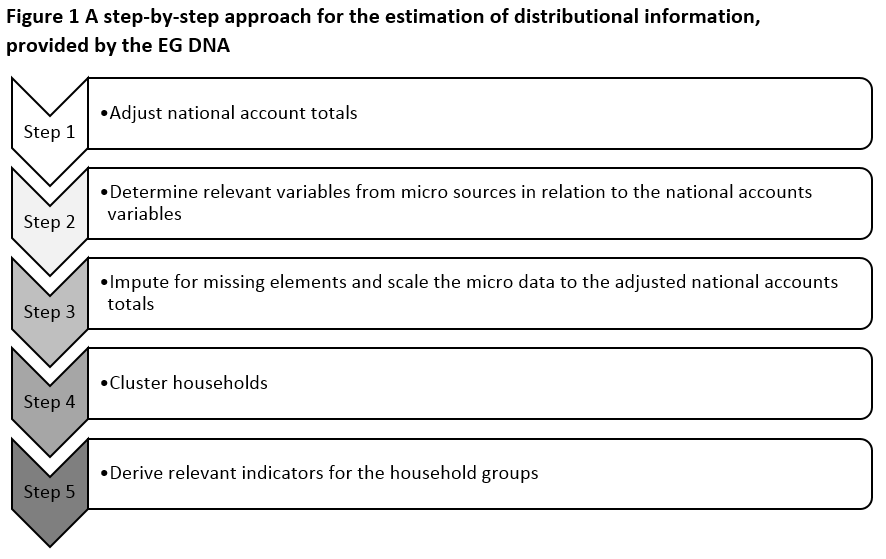
Description for Figure 1
Step 1. Adjust national account totals.
Step 2. Determine relevant variables from micro sources in relation to the national accounts variables.
Step 3. Impute for missing elements and scale the micro data to the adjusted national accounts totals.
Step 4. Cluster households.
Step 5. Derive relevant indicators for the household groups.
4 Adjusting the national accounts totals
4.1 National Balance Sheet Accounts
The NBSA are statements of the non-financial assets owned/used in the economy and of the financial claims outstanding (financial assets and liabilities) among the economic units in the economy. They consist of the national balance sheet for the country as a whole, as well as the underlying sector balance sheets. At the core of the NBSA are assets and liabilities and the concepts of wealth and net worth.
The DHEA focusses specifically on the household sector of the national balance sheet. This covers the assets, liabilities, and net worth (including some sub-categories) of all households in Canada.
4.2 Adjustments
The OECD recommends isolating the household sector for distributional analysis; a process that may require adjusting the National Accounts sector total if it has been aggregated with the NPISH sector.
Prior to the comprehensive revision in 2012, there were three main resident institutional sectors in the Canadian System of National Accounts (CSNA): the persons and unincorporated business sector, the corporate sector and the government sector. The persons and unincorporated business sector included NPISH, credit unions, life insurance companies, fraternal organizations and collective investment schemes such as pension plans and mutual funds. Due to data limitations, this sector also encompassed activities of Indigenous governments.
With the 2012 comprehensive revision, the CSNA adopted the basic SNA institutional sectoring detail throughout the sequence of integrated accounts. The former persons and unincorporated business sector was split between households and non-profit institutions serving households.
Given this work was already done to isolate the household sector, adjustments to the current NBSA data were not needed.
5 Micro-data source and variables
5.1 Survey of Financial Security
The micro-data source identified for the majority of distributions of net worth and their components is the SFS. The purpose of the survey is to collect information from a sample of Canadian families on their assets, debts, employment, income and education. This helps in understanding how family finances change because of economic pressures. The SFS provides a comprehensive picture of the net worth of Canadians. Information is collected on the value of all major financial and non-financial assets and on the money owing on mortgages, vehicles, credit cards, student loans and other debts. A family’s net worth is defined as the value of a family’s assets minus their debt and can be thought of as the amount of money they would be left with if they sold all of their assets and paid off all of their debts.
The SFS is a sample survey with a cross-sectional design. It had been conducted on an occasional basis, in 1999, 2005, and 2012, and since 2016 is undertaken triennially. In 2019, the SFS was once again collected and incorporated into the DHEA with the September 2021 release. The SFS covers the population living in the ten provinces of Canada. Within the provinces, certain groups are excluded (for instance, persons living on reserves or other Indigenous settlements and chronic care patients living in hospitals or nursing homes), which represent about 2% of the population.
Over the years, the SFS sample size and design have varied. The initial sample size was approximately 23,000 dwellings in 1999, 9,000 dwellings in 2005, and about 20,000 dwellings in 2012 and later reference years. In 1999, 2012, 2016 and 2019, provincial estimates were targeted but, with the sample size reduced significantly for budgetary reasons in 2005, that iteration of the survey focused on producing reliable estimates at the regional level.
Data are generally collected directly from respondents, while in some cases additional information is extracted from administrative files and derived from other Statistics Canada surveys and other sources via record linkage. Examples include the use of personal tax data records and regulatory information on the terms and conditions of employer-sponsored pension plans. Interviews are conducted via Computer-Assisted Personal Interviewing (CAPI) with an average interview length of approximately 45 minutes.
The survey is not mandatory and the response rates were 68.6%, 70.3% in 2012 and 2016 respectively, and 59.4% in 2019.
More information can be found on the Statistics Canada website under Definitions, data source and methods for SFS (survey number 2620) and tables 11-10-0016-01, 11-10-0049-01 and 11-10-0057-01.
5.2 Mapping and concordance
The full NBSA are comprised of 102 categories and sub-categories that contain all types of assets, liabilities and net worth in the economy. The DHEA data contain 11 of these categories. The NBSA categories were simplified for multiple reasons. One reason is that some types of assets and liabilities are not applicable in the household sector. Another reason is related to the quality of distributions that will be discussed in more detail in subsequent sections of this paper.
According to the United Nations Economic Commission for Europe (UNECE), “conceptually, macro and micro statistics on household income have much in common. However, there are significant differences in the objectives and purposes of the two datasets, in their coverage and the data sources used to compile them, and because of practical data reporting or estimation issues for individual households” (UNECE 2011). The concordance process allows for the identification of areas of conceptual difference between micro- and macro-data and provides an indicator of the suitability of specific micro-data variables as distributors of macro components.
The categories from the NBSA chosen for the DHEA are laid out in Table 1 below. The coverage ratios are shown for the SFS in 2012, 2016 and 2019, the years used to produce the DHEA wealth distributions based on the fourth quarter of each year from 2010 to 2019. These categories contain sufficient detail for analysis of household financial well-being and are the categories for which a suitable variable (or combination of variables) from the SFS has been identified. The concordances found in Table 1 are built by mapping variables from the SFS to a condensed version of the NBSA; the detail of which variables from each source were used to create this table are found in Table 2. Some details relating to the mapping in Table 2 are in sections 5.2.1 to 5.2.2.
| SFS | NBSA | Coverage (SFS/NBSA) |
|
|---|---|---|---|
| millions of dollars | percent | ||
| 2019 | |||
| Total assets | 13,556,182 | 14,080,399 | 96.3 |
| Financial assets | 6,613,501 | 7,512,709 | 88.0 |
| Life insurance and pensions | 2,513,121 | 2,830,004 | 88.8 |
| Other financial assets | 4,100,380 | 4,682,705 | 87.6 |
| Non-financial assets | 6,942,681 | 6,567,690 | 105.7 |
| Real estate | 6,264,424 | 5,800,658 | 108.0 |
| Other non-financial assets | 678,257 | 767,032 | 88.4 |
| Total liabilities | 1,866,265 | 2,382,730 | 78.3 |
| Mortgage liabilities | 1,507,421 | 1,549,938 | 97.3 |
| Other liabilities | 358,844 | 832,792 | 43.1 |
| Net worth (wealth) | 11,689,917 | 11,697,669 | 99.9 |
| 2016 | |||
| Total assets | 11,980,597 | 12,398,790 | 96.6 |
| Financial assets | 5,838,388 | 6,465,234 | 90.3 |
| Life insurance and pensions | 2,317,797 | 2,438,018 | 95.1 |
| Other financial assets | 3,520,591 | 4,027,216 | 87.4 |
| Non-financial assets | 6,142,209 | 5,933,556 | 103.5 |
| Real estate | 5,537,216 | 5,237,839 | 105.7 |
| Other non-financial assets | 604,993 | 695,717 | 87.0 |
| Total liabilities | 1,755,045 | 2,100,634 | 83.5 |
| Mortgage liabilities | 1,416,565 | 1,369,881 | 103.4 |
| Other liabilities | 338,481 | 730,753 | 46.3 |
| Net worth (wealth) | 10,225,552 | 10,298,156 | 99.3 |
| 2012 | |||
| Total assets | 9,367,532 | 9,457,510 | 99.0 |
| Financial assets | 4,666,076 | 4,861,470 | 96.0 |
| Life insurance and pensions | 1,871,134 | 1,894,943 | 98.7 |
| Other financial assets | 2,794,942 | 2,966,527 | 94.2 |
| Non-financial assets | 4,701,456 | 4,596,040 | 102.3 |
| Real estate | 4,186,037 | 4,020,480 | 104.1 |
| Other non-financial assets | 515,418 | 575,560 | 89.6 |
| Total liabilities | 1,337,071 | 1,733,129 | 77.1 |
| Mortgage liabilities | 1,029,811 | 1,101,942 | 93.5 |
| Other liabilities | 307,261 | 631,187 | 48.7 |
| Net worth (wealth) | 8,030,461 | 7,724,381 | 104.0 |
|
Note: NBSA estimates include the territories. Source: Statistics Canada, Distributions of Household Economic Accounts, 2021. |
|||
| Category | SFS variables | NBSA variables |
|---|---|---|
| Total assets |
|
|
| Financial assets |
|
|
| Life insurance and pensions |
|
|
| Other financial assets |
|
|
| Non-financial assets |
|
|
| Real estate |
|
|
| Other non-financial assets |
|
|
| Total liabilities |
|
|
| Mortgage liabilities |
|
|
| Other liabilities |
|
|
| Net worth (wealth) |
|
|
| Source: Statistics Canada, Distributions of Household Economic Accounts, 2021. | ||
5.2.1 Conceptual differences – valuables and collectibles
Valuables and collectibles are not an observed category in the NBSA and are not a part of the macro accounts asset boundary. Therefore, in order to align the micro source with the macro source, the value of valuables and collectibles is not included in the SFS total for net worth and non-financial assets.
5.2.2 Conceptual differences – other liabilities
The category with the lowest coverage ratio is ‘other liabilities’. The main reason for the under coverage of this category is due to the conceptual definition of credit card debt, which is mapped to this category. The SFS asks respondents to report the amount of credit card debt still owing on the last bill excluding new purchases, while the NBSA reports the total balance outstanding at a specific point in time. The difference reflects the fact that many households use credit cards for consumption and pay off their balance at the end of each period.
6 Clustering households
6.1 Unit of analysis: the household
The unit of analysis chosen for the DHEA is the household, defined by the OECD as “either an individual person or a group of persons who live together under the same housing arrangement and who combine to provide themselves with food and possibly other essentials of living” (OECD 2013a). The SFS data is available at the family unit level, which is comprised of unattached individuals and economic families defined as “a group of two or more persons who live in the same dwelling and are related to each other by blood, marriage, common-law or adoption” (Statistics Canada 2020-12-21). For the DHEA project, the economic family units have been aggregated to the household level by combining economic families that reside at the same address, which creates a unit definition that includes groups of people who share resources but are not necessarily related by blood, marriage, common-law or adoption. This brings the SFS data as close as possible to the OECD definition of household.
6.2 Distribution categories
DHEA estimates for assets, liabilities and net worth include eight separate distribution variables. Households are grouped by province, age group, household type (multiple-person vs. one-person), housing tenure, equivalized household disposable income quintile, main source of household income, generation, and household wealth quintile. Province, age group, household type and housing tenure groupings are based on definitions used in the SFS. When possible, the distribution variables are crossed together to give more detailed distributions. In particular, the DHEA also includes cross-tabulated distributions of the totals for assets, liabilities and net worth that include region by age group, region by equivalized household disposable income quintile, and equivalized household disposable income quintile by age group.
6.2.1 Province and region
The province represents that of the principal residence of the household. Household members who are temporarily away from their principal residence, for instance for work or study, are included in the province of their principal residence.
As well, the region is defined by aggregating provinces into the following five groups: Atlantic (Newfoundland, Nova Scotia, Prince Edward Island, and New Brunswick), Quebec, Ontario, Prairies (Manitoba, Saskatchewan, and Alberta), and British Columbia.
6.2.2 Age group
Households are grouped by age group according to the age of the major income earner as identified by the SFS. This differs from the OECD definition of a reference person for a household, which requires applying a number of characteristic criteria to each member of each household.
The age group categories used are: under 35, 35 to 44, 45 to 54, 55 to 64, and 65 and over.
6.2.3 Household type
Grouping by household type is done according to a simplified definition of household composition, with only two categories: households composed of one person and households composed of more than one person. The OECD recommends that, in addition to household size, the household type category should be cross-referenced by age and family composition, including marital status and presence of dependent children. The feasibility of grouping households by size, age and family composition will be reviewed as the methodology is further developed.
6.2.4 Housing tenure
Housing tenure is identified according to whether a principal residence is owned, with or without a mortgage, or rented. While rental costs for a tenant may be fully or partially subsidized, such a distinction is not identified for this category.
6.2.5 Equivalized household disposable income quintile
The household disposable income concept is unique to the SNA and is not measured directly in the SFS. While the estimates of wealth are not equivalized, the breakdown by income quintile is based on an equivalized income concept to reflect differences in household size and composition. In order to assign SFS households to disposable income quintiles, equivalized household disposable income must first be estimated for each household as follows:
- The SNA household disposable income aggregate is broken down into components (for example compensation of employees, transfers to and from other sectors, etc.) for which corresponding variables or proxies can be found on the SFS. The SFS income data is obtained from T1 income tax returns from Canada Revenue Agency (CRA) for the year prior to the survey year. When this data is not detailed enough to correspond to SNA household disposable income components, additional information is obtained from other tax files such as the Annual Income Estimates for Census Families and Individuals, commonly called the T1 Family File (T1FF) (see Statistics Canada (2021-07-14)) and the T4A supplementary file.
- For each income component, the SNA aggregate value is distributed over SFS households according to the value of the corresponding SFS variable or proxy. Survey weights are taken into account when calculating each household’s share of the component.
- For each household, the distributed components are summed up to calculate the household’s estimated disposable income.
- A final adjustment is done in order to equivalize the household disposable income. It consists of dividing the household disposable income by the number of consumption units for each household. This adjustment is based on the OECD-modified equivalence scale, which assigns a value of 1 to the first adult, 0.5 to each additional person aged 14 and over, and 0.3 for all children under 14.
The result is a new income variable for each SFS household, more closely aligned with the SNA concept of household disposable income than the available measure of after-tax income. Household equivalized disposable income is nevertheless highly correlated with equivalized after-tax income excluding capital gains, with a coefficient of correlation of 91.1% in 2012, 90.4% in 2016 and 92.8% in 2019.
Once every SFS household has been assigned an equivalized household disposable income, the households are grouped into equivalized household disposable income quintiles, which again are calculated taking into account the weights.
6.2.6 Main source of household income
The categories within the main source of household income are wages and salaries, self-employment income (i.e., farm and non-farm self-employment income, excluding rental income), net property income (i.e., interest and other investment income received less interest paid), pension benefits from corporations and governments, and other transfers (e.g., government social assistance, etc.).
6.2.7 Generation
Households are grouped into generation according to the birth year of the major income earner in the household as identified by the SFS. The generation categories used are: pre-1946 for those born before 1946, baby boom for those born between 1946 and 1964, generation X for those born between 1965 and 1980 and millennials for those born after 1980. Note that generation Z (for those generally born after 1996) has been combined with the millennials as their sample size is relatively small.
6.2.8 Household wealth quintile
Households are grouped by wealth quintile according to their total household net worth. Wealth quintiles group households into five equal parts, ranked from lowest to highest, each representing 20% of the total number of households in the economy. Contrary to the equivalization adjustment applied to disposable income quintiles, as described in section 6.2.5, wealth quintiles are not adjusted to account for differences in household size and composition. As noted in the literature, for inter-household comparison purposes, accounting for differences in the capacity of a household to consume wealth based on its size and composition at a given point in time may not be appropriate, since wealth tends to be consumed gradually over the life course. According to the OECD:
“Wealth is a stock of assets that is available to support consumption in the future, especially during retirement. When comparing households’ wealth as an indicator of economic well-being in terms of potential future consumption, consideration needs to be given to which household members are likely to benefit from that wealth. Of particular interest are households containing children. The children are likely to leave the household before the wealth of the household is used to support household consumption during retirement. Therefore, for this type of analysis, it does not seem relevant to equivalise wealth on the basis of the economies of scale in current consumption experienced with the current household structure. Rather, analysis of wealth should focus on examining data classified by life cycle group. Such a focus is consistent with the expectation that wealth is often built up during a person’s working life and then run down during retirement.” (OECD 2013b)
7 Deriving indicators in survey years
The SFS is the main source of distribution information for the DHEA for wealth. However, the SFS has been an occasional survey in the past and is triennial since 2016. This leaves gaps that need to be filled in order to produce a series of distributions in non-survey years. The methodology for deriving these distributions is two-fold, with a simpler, more direct approach being used in survey years and a calibration-based modelling approach in non-survey years. Throughout this section and the next two, descriptions will be given to show how much each step of the process modifies the estimates.
This section describes the first part of the methodology used to populate the tables in survey years. It consists of reweighting the SFS, scaling to NBSA totals, and then obtaining distribution estimates from the resulting data set. As of the September 2021 set of distributions, this methodology is used for survey years 2012, 2016, 2019 and, going forward, for every available survey year thereafter.
The next step, described in section 8, is to derive wealth measures for non-survey years using a modelling approach. After this is done, estimates for survey years and non-survey years are put together and adjustments are made to the estimates. First, estimates in survey years are adjusted in order to avoid introducing turning points when compared with the modelled estimates in adjacent non-survey years. Then adjustments for coherence and for the Northern territories of Canada are applied. This process is described in section 9.
7.1 Weight adjustments
The SFS weights currently used for the DHEA differ slightly from the version used to publish estimates obtained directly from the survey. The SFS sample is reweighted to reduce the impact of certain influential records and to take into account population control totals more closely related to the analytical categories of the DHEA.
The first step of the DHEA reweighting process is an adjustment to the weights of influential households that contribute significantly to net worth. Influential units can lead to unstable estimates and for this reason are often treated by adjusting their weights downward. Influential households, particularly in the lower income quintiles, are identified on the SFS samples and their weights are adjusted downward.
Following the weight adjustment for influential households, the SFS samples are recalibrated to population totals. Calibration consists of adjusting the weights of the sampled units so that estimates from the survey coincide with known totals at the population level. Potential benefits of calibration are consistency between the survey estimates and the known population totals, reduction of non-sampling errors, such as non-response errors and coverage errors, and improvement in the accuracy of estimators. The calibration totals used are estimates of counts for the sampled population based on projections from Statistics Canada’s Census of the Population, and are produced by Statistics Canada’s Demography Division. The totals used include counts of individuals by sex and age group categories, counts of households by household size, and counts of economic families by family size for select family sizes within provinces. The calibration methods used are as described in Deville and Sarndal (1992) and these methods are implemented in Statistics Canada’s G-EST software, which is described in Statistics Canada (2018-10).
These two reweighting steps, which together produce DHEA-specific weights, are part of the usual SFS weight calculation process that have been adjusted to align more closely with the DHEA analytical categories. This reweighting process is also used as a model for non-survey years, as described in section 8.1.
7.2 Adjustment for the elderly institutionalized population
The SFS excludes collective dwellings from its sample; in particular, nursing homes and residences for seniors are not sampled in the SFS. In order to account for the institutionalized elderly population, an adjustment is made to the DHEA wealth distributions. Prior to the June 2020 DHEA release, the institutionalized elderly population was accounted for in the DHEA income and consumption tables since this population is included in the Social Policy Simulation Database and Model (SPSD/M), but not the DHEA wealth tables. Globally, the institutionalized elderly population amounts to less than 1.3% of the Canadian population.
In order to ensure comparability between with DHEA income and consumption tables and the DHEA wealth tables, the adjustment made for the institutionalized elderly population follows a similar methodology to that used in the SPSD/M. Since no wealth data is collected for the institutionalized elderly population, the adjustment made is based on the assumption that those living in nursing homes or seniors residences are similar to individuals not in institutions who are aged 65 or older, live alone and are not in the labour force. The adjustment amounts to increasing the weights of these individuals on the SFS. The amount by which the weights are adjusted is based on Census counts of the institutionalized elderly population by province, age and sex. In order to account for the fact that this population is not living in their own home, adjustments are also made to certain asset and debt variables, such as those related to the principal residence.
7.3 Scaling to the National Balance Sheet Accounts
Following the methodology recommended by the OECD EG DNA, the survey data then is scaled to NBSA totals. Using these DHEA-specific weights, the SFS micro-data for every survey year, 2012, 2016 and 2019 in this case, are scaled. First, variables for asset and liability categories at the most granular level are scaled to the adjusted national accounts totals according to the concordance table in section 5.2. Subsequently, the values for the aggregate categories of assets and liabilities and for net worth are recalculated based on these scaled values for the granular-level categories of which they are composed.
7.4 Distribution estimates
For each of the DHEA tables, the total values of net worth and of each of the asset and liability sub-categories for each distribution category are estimated from SFS using the scaled values and the DHEA-specific weights.
The precision of the DHEA estimates in survey years is inherently linked to the precision of the SFS estimates. Measures of sampling error in the form of coefficients of variation (CVs) for SFS years are in the appendix in Tables 5 to 15. The CVs range from 1.6% to 12.4% for total net worth, from 1.5% to 11.7% for total assets, and from 1.8% to 14.5% for total liabilities among the provinces, age groups, household types, housing tenures, income quintiles, main sources of household income, generations and wealth quintiles.
8 Deriving indicators in non-survey years
Since the SFS is not undertaken annually, a different methodology is required to derive wealth measures for the DHEA in years for which survey information is not available. Without a direct measure of net worth and its components, the non-survey years must be modelled.
In previous versions of the DHEA, two modelling approaches were used: one based on calibration and another based on area-level models. More information on the methodology for these earlier releases can be found in Statistics Canada (2017-03-15, 2018-03-22). As of the March 2019 release (2019-03-27), a calibration-based approach has been exclusively used. Though the calibration and area-level model approaches are different mathematically, both often yielded similar distribution estimates for non-survey years.
8.1 Modelling using recalibration
The modelling approach used in this release is based on calibration. This approach is similar to the weight adjustments described in section 7.1. Starting with the influential value adjusted survey weights, the weights are recalibrated to demographic control totals for non-survey years. This recalibration adjusts the weights of the sampled units so that estimates from the survey coincide with these population totals for non-survey years, in essence adjusting the survey weights to reflect demographic shifts.
Once the weights of the SFS samples are adjusted to reflect demographic shifts, the SFS micro-data is scaled to the adjusted national accounts totals, as described above in section 7.3. Estimates for net worth and its components are then obtained for non-survey years by aggregating the micro-data and using the adjusted weights, as in section 7.4. This process is done once for every survey year giving three series of estimates for the time period between 2010 and 2020, one using the 2012 SFS, one using the 2016 SFS and another using the 2019 SFS.
The series based on SFS 2012 is used for estimates for 2010 to 2012. For 2013 to 2015, the series are combined by linearly interpolating between the series. For example, for 2013, the combined estimate is calculated as ¾ × estimate from SFS 2012 recalibrated to 2013 + ¼ × estimate from the SFS 2016 recalibrated to 2013. Similarly, linear interpolation is applied to the 2016 SFS and 2019 SFS series to derive estimates from 2017 to 2018, while SFS 2019 is used to produce estimates for 2019 and 2020.
8.2 Performance of the recalibration approach
Tables 16 to 18 in the appendix show how the modelled distributions obtained by the recalibration approach compare to the SFS distributions in 2019, 2016, 2012, 2005, and 1999 for select components of net worth. The range of the absolute differences by category between the SFS distribution and modelled distribution is shown as a measure of distance between the SFS distributions and those obtained by modelling.
Before adopting a calibration-only approach, the results of the previously-used area-level models and the calibration models were compared and the strengths and weaknesses of each approach were considered (Wu and Boulet 2018). This comparison was done on the set of tables available as part of the March 2018 dissemination. Both methods are designed to ensure that the distributions in survey years concord with the SFS estimates. As a result, when the number of years between surveys is short, both approaches give similar results. In fact, once the final steps described in the next section were conducted, the difference in the share held by each group was less than 1% in nearly all cells of the tables.
The main advantage of the area-level model approach is that it can theoretically capture trends in wealth that are related to income. However, it was not clear that in practice area-level modelling was better able to capture the effect of large events, such as the 2008 recession. Given that the area models use income data, one might expect for example that the area models would show the wealth of the lowest income quintile being affected differently by the recession than the wealth of the highest income quintile. Unfortunately, the estimates are too noisy to distinguish any differences.
On the other hand, the calibration approach has important practical advantages. Principally, it is much less time and resource intensive than the area-level model approach in which models must be built individually for each distribution category. A by-product of this advantage is that it makes it more practical to build tables for additional distribution categories as has been done since adopting this modelling approach. Furthermore, the area-level approach depended on auxiliary information that is only available a year and a half after the end of the reference period whereas the control totals required for the calibration approach are available without such a time lag.
Given the significant practical advantages to the calibration approach, together with the similarity of the estimates coming from the two approaches, it was decided to adopt the calibration only approach for the March 2019 release and the following releases.
9 Adjustments to the final tables
9.1 Adjustments to survey years
After combining the two series of estimates obtained by recalibration, small adjustments are made to estimates in survey years in order to avoid introducing turning points at 2012, 2016 and 2019 when compared with the modelled estimates in adjacent non-survey years. A three-point centred weighted moving average is applied to the combined series in 2012, 2016 and 2019.
After applying these adjustments to the survey year data, the row and column sums of the resulting tables are not coherent in survey years. The sum of the distribution categories are not equal to the NBSA totals; in other words, the row sums are not coherent. As well, the relationships between assets, liabilities and net worth are not respected; in other words, the column sums are not coherent. Additionally, the sum of data in the cross-tabulation tables may not be exactly equal to the data in the one-dimensional tables.
An adjustment process is required to ensure consistency within and between the tables. This type of adjustment goes by many names: raking, balancing, and reconciliation. It re-establishes the relationships between net worth, assets, and liabilities categories while ensuring that the sum of the distribution categories are kept equal to the NBSA total and leaves the NBSA totals untouched. A key characteristic of raking is that it ensures that specified relationships are respected while minimizing the change to individual cells of the table.
The raking methods used are derived from the Dagum and Cholette (2006) regression-based approach and are further described in Quenneville and Fortier (2012), and the references therein. The procedures are implemented in PROC TSRAKING and the GSeriesTSBalancing macro in Statistics Canada’s G-Series software. They are described in Statistics Canada (2016-04) and the references therein, and can be obtained by contacting statcan.g-series-g-series.statcan@canada.ca.
The magnitude of the smoothing and raking adjustments to the internal cells of the wealth tables are in Table 3. These factors are calculated as values after raking divided by values after combining the estimates from recalibration. These adjustments are generally close to 1, indicating that smoothing and raking the tables does not result in major changes to the distributions.
| Range of adjustments | Proportion of adjustments of 1% or less (in percent) | |
|---|---|---|
| Province | Note ...: not applicable | Note ...: not applicable |
| Age group of major income earner | [0.97, 1.03] | 78 |
| Generation of major income earner | [0.98, 1.06] | 61 |
| Household type | [0.99, 1.01] | 98 |
| Housing tenure | [0.98, 1.04] | 79 |
| Equivalized household disposable income quintile | [0.98, 1.03] | 78 |
| Main source of household income | [0.95, 1.16] | 63 |
| Household wealth quintile | [0.94, 1.07] | 65 |
| Region by age group of major income earner | [0.97, 1.08] | 66 |
| Region by equivalized household disposable income quintile | [0.92, 1.07] | 43 |
| Equivalized household disposable income quintile by age group of major income earner | [0.93, 1.13] | 42 |
|
... not applicable Source: Statistics Canada, Distributions of Household Economic Accounts, 2021. |
||
9.2 Other adjustments
9.2.1 Quarterly wealth distributions
As the COVID-19 pandemic unfolded in Canada at the beginning of 2020, households experienced large changes in their economic well-being over a relatively brief period of time. To provide more timely information about the economic impacts of the pandemic on different households, this latest release includes wealth distributions on a quarterly basis starting with the 2020 reference year.
Based on distributions for liabilities as of the fourth quarter of reference year 2019 that are benchmarked to NBSA totals, quarterly projections of household liabilities are created using sub-aggregated data from Equifax Canada, a private consumer credit rating agency. Equifax credit registry include sub-annual data on the majority of household mortgage and non-mortgage credit transactions processed through more than 600 financial institutions across Canada (e.g., including banks, credit unions, mortgage financers, automobile dealers and financers, credit card companies, finance companies, and retailers), while coverage is relatively limited for alternative financial intermediaries (e.g., insurance providers, payday loan companies, etc.). Relative to NBSA benchmarks as of the fourth quarter of 2019, Equifax data represent 81.5% of total liabilities, including 84.0% of mortgage liabilities and 77.0% of non-mortgage liabilities.
Quarterly trends in household liabilities are available from Equifax Canada by type of credit product (e.g., mortgage, credit card, car loan, etc.) and demographic characteristic, including province, age of household head, generation of household head, and household composition. In contrast with the method used to identify household head within the DHEA, which is based on the major income earner (see section 6.2), a different method is applied for projections based on Equifax data. Due to the lack of income data within the credit registry, household head is determined by Equifax Canada by applying the following criteria:
- The household member who has an active mortgage or home equity line of credit (HELOC). If multiple or none of the members have an active mortgage or HELOC, then;
- The member who has the highest total credit limits for all credit products. If multiple members have equal total credit limits or none of them have credit, then;
- The member who is the oldest in the household. If age is equal for all members, then;
- The member who is listed first in the credit registry database for that household.
Relative to DHEA estimates for household liabilities as of the fourth quarter of reference year 2019, as indicated in Table 4, coverage for Equifax totals by province range from 64.4% to 96.8%, by age group from 66.1% to 105.8%, by generation from 59.0% to 118.1%, and by household composition from 66.7% to 148.4%.
| Total liabilities | Mortgage liabilities | Other liabilities | |
|---|---|---|---|
| percent | |||
| All households | 81.5 | 84.0 | 77.0 |
| Province | |||
| Newfoundland and Labrador | 79.4 | 86.2 | 71.2 |
| Prince Edward Island | 81.7 | 78.7 | 85.2 |
| Nova Scotia | 83.2 | 96.8 | 70.4 |
| New Brunswick | 78.7 | 84.0 | 73.9 |
| Quebec | 85.8 | 86.3 | 84.9 |
| Ontario | 82.9 | 83.8 | 81.1 |
| Manitoba | 71.0 | 71.0 | 71.0 |
| Saskatchewan | 73.3 | 79.9 | 64.4 |
| Alberta | 77.6 | 80.1 | 73.2 |
| British Columbia | 80.9 | 87.2 | 68.3 |
| Age group of major income earner | |||
| Under 35 years | 62.2 | 63.6 | 59.0 |
| 35 to 44 years | 80.1 | 80.8 | 78.2 |
| 45 to 54 years | 81.8 | 82.9 | 79.5 |
| 55 to 64 years | 92.6 | 106.4 | 77.1 |
| 65 years and over | 104.0 | 118.1 | 92.1 |
| Generation of major income earner | |||
| Millennials | 69.3 | 70.6 | 66.1 |
| Generation X | 82.1 | 83.1 | 79.7 |
| Baby boom | 93.3 | 105.8 | 79.7 |
| Pre-1946 | 95.1 | 101.9 | 90.0 |
| Household type | |||
| One-person household | 147.4 | 146.8 | 148.4 |
| Multiple-person household | 72.4 | 75.5 | 66.7 |
| Source: Statistics Canada, Distributions of Household Economic Accounts, 2021; Equifax. | |||
To derive quarterly debt distributions related to income, including equivalized household disposable income quintile and main source of household income, a matching exercise is applied to link SFS and Equifax wealth distributions with households covered within the SPSD/M. Using the results from a special run of the SPSD/M (Statistics Canada, 2020-10-14), sub-annual trends in disposable income by distribution category are derived from Labour Force Survey wage trends and administrative data on government Covid-19 economic relief measures. Further adjustments are also applied to ensure alignment with modelled distributions for government benefits (e.g., Canadian Emergency Relief Benefits from Employment and Skills Development Canada, etc.)
To ensure consistency of the quarterly trends in household liabilities observed from the credit registry data with the associated trends in non-financial assets to which those liabilities relate, corresponding adjustments are also applied to quarterly real estate asset values using distributional information from third parties on the housing market (Canada Mortgage and Housing Corporation 2021) and spending on consumer goods (Bank of Canada 2020).
As well, to more accurately reflect sub-annual demographic trends in the household population that are aligned with wealth and income, household counts benchmarked to distributions from Demography Division as of the 2019 reference year are grown on a quarterly basis starting in reference year 2020. Quarterly household counts are created using data available from the Equifax data and the SPSD/M, and are used to present wealth estimates by distribution category on an average dollars per household basis.
9.2.2 Territorial factor adjustments
An additional adjustment is applied to the DHEA wealth distributions by province and region to remove a portion of the national NBSA wealth control totals related to households in the territories. This adjustment is necessary as the SFS sample is drawn only from households in the ten provinces (see sections 5.1 and 10.2.2), while the published NBSA control totals are based on the total for all provinces and territories in Canada. Without this adjustment, and since the NBSA does not estimate wealth for the territories, DHEA estimates of wealth by province and region would be overestimated.
Since territorial wealth is not directly identifiable through existing data sources, a simplified adjustment is applied to the NBSA national control totals to adjust for territorial wealth. In particular, a fixed percentage is removed from each of the wealth categories based on SNA estimates for territorial net property income, scaled by average government bond yields and mortgage rates. The same percentage is removed for each province and region's wealth estimate. While the same percentage is used in any given year, this percentage can vary over time, depending on the growth in net property income relative to that for the national NBSA control totals. This simplified adjustment rests on the assumption that the territories have the same distribution as the total for the provinces included in the SFS sample.
9.2.3 Data quality adjustments
As well, as part of the DHEA data quality assessment process, adjustments are applied to some wealth distributions at the macro level to avoid introducing turning points in survey years or to avoid discrepancies with economic and demographic trends observed from other data sources, such as from surveys and government administrative data.
10 Sources of error
The DHEA are built by bringing together data from multiple sources. Each of these sources, as well as the way in which they are used and combined, are a potential source of gaps between the micro- and macro-level data. An overview of the sources of error for the DHEA wealth distributions is given below, categorized according to their source:
- national accounts totals;
- model;
- survey data.
A similar classification is found in Zwijnenburg (2016).
10.1 Quality of national accounts data
10.1.1 Quality of national accounts totals
The NBSA are estimated by using the most complete and high quality data sources available in order to establish benchmark estimates. This generally entails business surveys, administrative data files from the CRA, household survey files, information from pension funds, financial institutions and government public accounts. Data are analyzed for time series consistency, links to current economic events, issues arising from the source data, and finally with respect to coherence. It is not possible to produce an equivalent to national wealth or national net worth; nor is it possible to construct a balance sheet for the household sector, except periodically from household surveys. However, certain sub-sectors of the NBSA are largely comparable to estimates produced by source data divisions (e.g., pension funds, levels of government).
10.1.2 Quality of the adjustments to the national accounts totals
As previously mentioned, the adjustment to isolate the household sector from the NPISH sector was implemented in 2012. Work to build the NPISH sector began with the creation of a more broadly defined satellite account of non-profit institutions and volunteering, first released in 2004. The NPISH portion of this broader non-profit sector was implemented in the core SNA in 2012, with estimates built from a variety of sources including administrative files on registered charities and other non-profit institutions. A range of statistical improvements to better define the universe and account for measurement deficiencies were undertaken in addition to the sectoring changes. These included delineating the purchases of households from the NPISH sector. Revised industry and final demand estimates were correspondingly introduced in the supply-use framework.
10.2 Quality of survey data
10.2.1 Sampling error
Sampling error is inevitable in any sample survey and occurs because data is collected and inferences are made from a sample, rather than the entire population. The sampling error is measured by estimating the extent to which sample estimates would vary over all possible samples that could have been selected with the same design and sample size. The magnitude of the sampling error is affected by several factors: the inherent variability in the population of the characteristic being measured, the sample size, the sample design, and the response rate. With its smaller size, the 2005 SFS has a larger sampling error than do the other years of SFS.
The CV is a common measure of sampling error and can be used as one indicator of the accuracy of the estimates. It is defined as the ratio of the estimated standard error of the estimate to the value of estimate itself. The CVs for estimates of totals of net worth and its components from the SFS for survey years 2012 and later are in the appendix in Tables 5 to 15.
10.2.2 Coverage error
Coverage errors are omissions, erroneous additions, duplicates and errors of classification of units in the survey frame. They can create biased estimates and the impact can vary for different sub-groups of the population.
For the DHEA, the population targeted by the SFS and the NBSA totals differ. In particular, the territories are excluded from SFS, as are about 2% of persons in the provinces who are difficult to survey for a variety of reasons.
Due to a lack of information on the value of assets and liabilities for households in the territories and for the elderly institutionalized population, the DHEA applies simplistic adjustments to include these populations in its estimates. These adjustments are described in sections 7.2 and 9.2. More accurate estimates for the wealth of these populations may be derived in the future if data from alternative data sources covering these population becomes available.
10.2.3 Non-response error
There are two kinds of non-response: total non-response, not answering the whole survey, and item non-response, not answering some questions. In the SFS, this type of error is addressed by using follow-up procedures to minimize non-response, by weighting that takes into account non-response, and by imputation.
10.2.4 Measurement and processing error
Measurement error, also called response error, is the difference between the recorded response to a question and the “true” value. Measurement error can be caused by misunderstanding on the part of the respondent or the interviewer. Processing is required to transform survey responses into a form suitable to tabulation and analysis and may be a source of error.
10.3 Quality of the models used for non-survey years
In non-SFS years, the DHEA wealth distributions must be modelled. As such, their quality of the estimated distributions depends both on the quality of the auxiliary data on which the models are built and on the strength of the models themselves.
10.3.1 Quality of auxiliary data sources
The auxiliary data source used for the recalibration approach are demographic projections of person and household counts based on Statistics Canada’s Census of the Population. These projections cover the same sampled population as the SFS and exclude the same segments of the population (see section 10.2.2), and use the same household and family concepts as the SFS. They are of high quality and are used for the calibration of most social surveys at Statistics Canada.
10.3.2 Quality of the models
Models are a fundamental component of the DHEA wealth distributions methodology and, as with any model, they can only reflect the trends for net worth distributions that are related to trends in the auxiliary data. In this case, since the recalibration approach has been adopted as of the March 2019 release, this means trends related to demographics only. As discussed in section 8.2, when more than one survey year is available and when gaps between survey years are relatively short, this has a small impact on the final estimates. However, revisions to the years following the last available survey year should be expected to be greater than revisions to prior years. It should also be noted that the strength of the relationship between wealth distributions and demographics varies by the household category. This is reflected in the comparisons of the modelled and SFS distributions in the appendix in section 11.2.
10.4 Combining these sources
The DHEA brings together data from many difference sources and, so, it is not surprising that conceptual differences between micro- and macro-data sources are a major challenge. The methodology put forth in this paper and used to produce the DHEA wealth distributions is comprised of multiple steps (reconciliation of micro and macro concepts, modelling through recalibration, raking). Throughout these steps, the errors may accumulate or cancel out.
11 Appendix
11.1 Sample error coefficients of variation for the Survey of Financial Security, 2012 and 2016
The following tables contain the sampling error CVs, or ranges of CVs, from the SFS. These CVs are based on the SFS and do not include the steps of reweighting and scaling to the NBSA.
| Province | ||||||||||
|---|---|---|---|---|---|---|---|---|---|---|
| Newfoundland and Labrador | Prince Edward Island | Nova Scotia | New Brunswick | Quebec | Ontario | Manitoba | Saskatchewan | Alberta | British Columbia | |
| coefficient of variation | ||||||||||
| 2019 | ||||||||||
| Total assets | 5.6 | 9.2 | 6.0 | 4.9 | 3.0 | 2.7 | 4.7 | 6.0 | 3.6 | 3.2 |
| Financial assets | 8.2 | 11.5 | 7.9 | 7.2 | 4.3 | 3.6 | 6.7 | 8.5 | 5.8 | 5.5 |
| Life insurance and pensions | 7.8 | 9.2 | 7.2 | 7.9 | 3.9 | 3.4 | 6.4 | 6.9 | 4.8 | 4.8 |
| Other financial assets | 15.8 | 20.0 | 14.6 | 12.3 | 7.0 | 5.5 | 11.2 | 12.0 | 7.6 | 8.0 |
| Non-financial assets | 4.6 | 8.3 | 7.4 | 5.0 | 2.7 | 2.9 | 5.0 | 4.4 | 2.9 | 3.1 |
| Real estate | 5.2 | 9.6 | 8.1 | 5.6 | 3.0 | 3.1 | 5.6 | 5.0 | 3.2 | 3.3 |
| Other non-financial assets | 5.8 | 6.9 | 6.5 | 6.6 | 2.8 | 3.3 | 5.6 | 5.1 | 3.5 | 5.6 |
| Total liabilities | 7.2 | 8.0 | 8.1 | 6.0 | 4.1 | 3.5 | 6.9 | 5.5 | 3.2 | 4.9 |
| Mortgage liabilities | 9.1 | 10.9 | 10.8 | 7.6 | 4.7 | 3.9 | 7.7 | 6.8 | 3.7 | 5.6 |
| Other liabilities | 7.2 | 10.1 | 7.8 | 7.0 | 6.0 | 4.8 | 11.3 | 7.3 | 5.7 | 8.6 |
| Net worth (wealth) | 6.4 | 10.1 | 6.6 | 5.7 | 3.3 | 3.0 | 5.0 | 6.8 | 4.3 | 3.6 |
| 2016 | ||||||||||
| Total assets | 5.5 | 6.4 | 4.3 | 4.4 | 3.0 | 2.3 | 3.9 | 5.2 | 3.8 | 3.1 |
| Financial assets | 7.6 | 9.1 | 6.0 | 5.5 | 4.0 | 3.5 | 5.3 | 7.2 | 5.9 | 4.5 |
| Life insurance and pensions | 7.8 | 8.0 | 7.2 | 7.5 | 3.4 | 2.9 | 5.7 | 5.5 | 4.6 | 3.9 |
| Other financial assets | 11.4 | 15.1 | 8.9 | 8.7 | 6.5 | 5.5 | 8.7 | 11.0 | 8.2 | 6.6 |
| Non-financial assets | 5.6 | 6.3 | 5.4 | 5.5 | 2.9 | 2.2 | 4.4 | 4.4 | 3.0 | 3.5 |
| Real estate | 5.9 | 7.2 | 6.2 | 6.3 | 3.2 | 2.3 | 4.8 | 5.0 | 3.4 | 3.6 |
| Other non-financial assets | 8.7 | 8.5 | 4.9 | 5.2 | 2.9 | 3.4 | 4.4 | 5.2 | 3.6 | 4.0 |
| Total liabilities | 7.8 | 9.5 | 7.1 | 8.1 | 4.1 | 2.9 | 6.9 | 5.7 | 4.3 | 4.4 |
| Mortgage liabilities | 10.4 | 11.8 | 9.4 | 9.9 | 4.9 | 3.2 | 8.1 | 6.8 | 5.0 | 5.0 |
| Other liabilities | 7.4 | 9.7 | 8.1 | 8.7 | 3.8 | 4.6 | 7.1 | 9.3 | 4.7 | 6.1 |
| Net worth (wealth) | 6.1 | 7.3 | 4.8 | 4.8 | 3.2 | 2.6 | 4.4 | 5.8 | 4.4 | 3.4 |
| 2012 | ||||||||||
| Total assets | 4.6 | 10.9 | 5.5 | 4.2 | 3.9 | 2.9 | 4.8 | 4.7 | 3.7 | 3.1 |
| Financial assets | 7.4 | 14.4 | 7.3 | 6.2 | 5.3 | 3.9 | 6.2 | 6.2 | 5.9 | 4.4 |
| Life insurance and pensions | 9.8 | 17.4 | 8.2 | 8.0 | 3.9 | 4.7 | 7.1 | 8.1 | 6.2 | 5.0 |
| Other financial assets | 10.6 | 20.5 | 11.0 | 11.0 | 8.9 | 5.6 | 10.2 | 9.3 | 8.0 | 6.6 |
| Non-financial assets | 5.4 | 10.3 | 4.8 | 3.5 | 3.7 | 3.3 | 5.0 | 5.2 | 3.8 | 4.1 |
| Real estate | 5.6 | 10.6 | 5.3 | 4.1 | 4.2 | 3.5 | 5.5 | 5.6 | 4.1 | 4.5 |
| Other non-financial assets | 8.0 | 11.3 | 5.6 | 6.2 | 3.4 | 3.6 | 6.2 | 8.4 | 3.4 | 4.0 |
| Total liabilities | 9.8 | 10.0 | 6.6 | 5.4 | 6.0 | 4.6 | 6.1 | 7.4 | 5.0 | 4.5 |
| Mortgage liabilities | 12.2 | 16.1 | 8.3 | 7.6 | 7.6 | 5.4 | 7.3 | 9.3 | 7.1 | 5.2 |
| Other liabilities | 8.0 | 13.2 | 8.3 | 5.6 | 6.2 | 5.8 | 7.9 | 7.7 | 7.5 | 6.8 |
| Net worth (wealth) | 5.7 | 12.4 | 6.1 | 4.9 | 4.1 | 3.1 | 5.3 | 5.3 | 4.3 | 3.4 |
| Source: Statistics Canada, Survey of Financial Security, 2012, 2016 and 2019. | ||||||||||
| Age group of major income earner | |||||
|---|---|---|---|---|---|
| Under 35 years | 35 to 44 years | 45 to 54 years | 55 to 64 years | 65 years and over | |
| coefficient of variation | |||||
| 2019 | |||||
| Total assets | 4.6 | 3.7 | 4.2 | 3.0 | 3.0 |
| Financial assets | 8.6 | 6.2 | 5.5 | 3.4 | 4.2 |
| Life insurance and pensions | 7.7 | 5.1 | 4.2 | 3.9 | 3.6 |
| Other financial assets | 10.6 | 9.3 | 8.9 | 4.9 | 5.7 |
| Non-financial assets | 4.6 | 3.7 | 4.1 | 4.0 | 2.9 |
| Real estate | 5.0 | 3.9 | 4.4 | 4.3 | 3.0 |
| Other non-financial assets | 4.2 | 4.1 | 3.3 | 4.3 | 3.9 |
| Total liabilities | 4.8 | 3.8 | 4.3 | 4.6 | 5.9 |
| Mortgage liabilities | 5.6 | 4.2 | 4.8 | 5.4 | 7.3 |
| Other liabilities | 5.4 | 5.3 | 6.0 | 6.6 | 7.9 |
| Net worth (wealth) | 5.7 | 4.4 | 4.7 | 3.2 | 3.1 |
| 2016 | |||||
| Total assets | 4.3 | 3.7 | 3.2 | 2.9 | 2.7 |
| Financial assets | 6.1 | 6.6 | 5.0 | 3.6 | 3.1 |
| Life insurance and pensions | 6.5 | 4.6 | 3.8 | 3.3 | 3.1 |
| Other financial assets | 8.1 | 10.1 | 8.1 | 5.8 | 4.1 |
| Non-financial assets | 4.8 | 3.3 | 3.1 | 3.2 | 3.0 |
| Real estate | 5.2 | 3.5 | 3.3 | 3.4 | 3.2 |
| Other non-financial assets | 4.9 | 3.4 | 3.4 | 3.8 | 3.3 |
| Total liabilities | 3.9 | 3.3 | 3.8 | 4.3 | 7.8 |
| Mortgage liabilities | 4.5 | 3.6 | 4.2 | 5.2 | 10.6 |
| Other liabilities | 4.5 | 4.4 | 5.8 | 4.4 | 6.0 |
| Net worth (wealth) | 5.5 | 4.4 | 3.6 | 3.1 | 2.7 |
| 2012 | |||||
| Total assets | 6.7 | 4.5 | 3.9 | 3.8 | 2.8 |
| Financial assets | 12.1 | 5.8 | 5.1 | 4.6 | 3.6 |
| Life insurance and pensions | 11.7 | 6.5 | 4.9 | 4.7 | 3.9 |
| Other financial assets | 15.6 | 7.9 | 7.5 | 7.2 | 5.2 |
| Non-financial assets | 5.4 | 5.0 | 4.0 | 4.1 | 3.6 |
| Real estate | 5.9 | 5.4 | 4.3 | 4.4 | 3.8 |
| Other non-financial assets | 6.0 | 4.1 | 3.9 | 3.9 | 4.2 |
| Total liabilities | 5.6 | 5.0 | 4.5 | 6.4 | 8.6 |
| Mortgage liabilities | 6.4 | 5.7 | 5.2 | 8.3 | 11.2 |
| Other liabilities | 5.8 | 5.5 | 6.7 | 7.0 | 11.2 |
| Net worth (wealth) | 8.5 | 5.2 | 4.2 | 3.8 | 2.8 |
| Source: Statistics Canada, Survey of Financial Security, 2012, 2016 and 2019. | |||||
| Generation of major income earner | ||||
|---|---|---|---|---|
| Pre-1946 | Baby boom | Generation X | Millennials | |
| coefficient of variation | ||||
| 2019 | ||||
| Total assets | 5.2 | 2.4 | 3.3 | 3.9 |
| Financial assets | 7.4 | 2.8 | 4.5 | 6.7 |
| Life insurance and pensions | 5.9 | 3.0 | 3.5 | 5.9 |
| Other financial assets | 9.6 | 3.9 | 7.1 | 8.6 |
| Non-financial assets | 4.6 | 3.0 | 3.3 | 3.7 |
| Real estate | 4.8 | 3.2 | 3.6 | 4.0 |
| Other non-financial assets | 7.1 | 3.1 | 2.7 | 4.2 |
| Total liabilities | 11.3 | 3.9 | 3.4 | 3.9 |
| Mortgage liabilities | 14.7 | 4.6 | 3.7 | 4.5 |
| Other liabilities | 14.5 | 5.3 | 4.7 | 4.4 |
| Net worth (wealth) | 5.3 | 2.5 | 3.7 | 4.8 |
| 2016 | ||||
| Total assets | 3.8 | 2.2 | 2.8 | 4.1 |
| Financial assets | 4.2 | 2.8 | 4.4 | 5.9 |
| Life insurance and pensions | 4.1 | 2.5 | 3.3 | 6.4 |
| Other financial assets | 5.5 | 4.3 | 7.0 | 7.8 |
| Non-financial assets | 4.1 | 2.4 | 2.7 | 4.5 |
| Real estate | 4.3 | 2.6 | 2.9 | 4.9 |
| Other non-financial assets | 4.4 | 2.8 | 2.7 | 4.6 |
| Total liabilities | 14.1 | 3.3 | 3.0 | 3.7 |
| Mortgage liabilities | 18.9 | 3.9 | 3.2 | 4.2 |
| Other liabilities | 9.2 | 3.9 | 4.2 | 4.3 |
| Net worth (wealth) | 3.7 | 2.3 | 3.2 | 5.2 |
| 2012 | ||||
| Total assets | 3.5 | 2.5 | 3.7 | 9.0 |
| Financial assets | 4.5 | 3.1 | 5.2 | 17.1 |
| Life insurance and pensions | 4.2 | 3.2 | 4.9 | 18.4 |
| Other financial assets | 6.5 | 5.0 | 7.2 | 21.5 |
| Non-financial assets | 4.0 | 2.6 | 4.1 | 6.9 |
| Real estate | 4.3 | 2.8 | 4.4 | 7.4 |
| Other non-financial assets | 3.6 | 2.9 | 3.3 | 8.5 |
| Total liabilities | 9.8 | 3.7 | 3.9 | 7.2 |
| Mortgage liabilities | 13.3 | 4.6 | 4.4 | 8.9 |
| Other liabilities | 12.3 | 5.2 | 4.2 | 6.7 |
| Net worth (wealth) | 3.5 | 2.7 | 4.4 | 11.7 |
| Source: Statistics Canada, Survey of Financial Security, 2012, 2016 and 2019. | ||||
| Household type | ||
|---|---|---|
| One-person household | Multiple-person household | |
| coefficient of variation | ||
| 2019 | ||
| Total assets | 3.6 | 1.7 |
| Financial assets | 4.6 | 2.5 |
| Life insurance and pensions | 5.2 | 2.1 |
| Other financial assets | 6.0 | 3.7 |
| Non-financial assets | 3.8 | 1.8 |
| Real estate | 4.1 | 1.9 |
| Other non-financial assets | 3.7 | 1.9 |
| Total liabilities | 5.8 | 2.1 |
| Mortgage liabilities | 6.9 | 2.4 |
| Other liabilities | 5.6 | 3.1 |
| Net worth (wealth) | 3.8 | 1.9 |
| 2016 | ||
| Total assets | 2.6 | 1.5 |
| Financial assets | 3.4 | 2.1 |
| Life insurance and pensions | 4.0 | 1.8 |
| Other financial assets | 4.7 | 3.3 |
| Non-financial assets | 2.8 | 1.5 |
| Real estate | 3.0 | 1.6 |
| Other non-financial assets | 4.0 | 1.6 |
| Total liabilities | 4.5 | 1.9 |
| Mortgage liabilities | 5.2 | 2.2 |
| Other liabilities | 4.9 | 2.5 |
| Net worth (wealth) | 2.7 | 1.6 |
| 2012 | ||
| Total assets | 4.8 | 1.7 |
| Financial assets | 6.4 | 2.3 |
| Life insurance and pensions | 6.0 | 2.5 |
| Other financial assets | 9.1 | 3.6 |
| Non-financial assets | 5.5 | 1.9 |
| Real estate | 5.9 | 2.0 |
| Other non-financial assets | 4.1 | 1.9 |
| Total liabilities | 9.6 | 2.3 |
| Mortgage liabilities | 11.9 | 2.8 |
| Other liabilities | 7.5 | 3.3 |
| Net worth (wealth) | 4.9 | 1.8 |
| Source: Statistics Canada, Survey of Financial Security, 2012. 2016 and 2019. | ||
| Housing tenure | |||
|---|---|---|---|
| Own with mortgage | Own without mortgage | Rent | |
| coefficient of variation | |||
| 2019 | |||
| Total assets | 2.4 | 2.7 | 5.8 |
| Financial assets | 3.5 | 3.4 | 6.7 |
| Life insurance and pensions | 3.2 | 3.3 | 6.3 |
| Other financial assets | 5.9 | 4.6 | 9.7 |
| Non-financial assets | 2.5 | 2.7 | 8.6 |
| Real estate | 2.6 | 2.8 | 13.1 |
| Other non-financial assets | 3.1 | 2.9 | 3.6 |
| Total liabilities | 2.3 | 6.7 | 6.7 |
| Mortgage liabilities | 2.4 | 11.6 | 15.4 |
| Other liabilities | 4.0 | 6.4 | 4.5 |
| Net worth (wealth) | 2.7 | 2.7 | 6.2 |
| 2016 | |||
| Total assets | 2.0 | 2.5 | 4.7 |
| Financial assets | 3.0 | 3.1 | 5.0 |
| Life insurance and pensions | 2.8 | 2.9 | 5.6 |
| Other financial assets | 5.1 | 4.2 | 6.8 |
| Non-financial assets | 2.1 | 2.6 | 7.7 |
| Real estate | 2.2 | 2.7 | 11.8 |
| Other non-financial assets | 2.6 | 2.8 | 4.0 |
| Total liabilities | 2.0 | 6.7 | 7.1 |
| Mortgage liabilities | 2.0 | 12.5 | 18.2 |
| Other liabilities | 3.3 | 4.9 | 4.2 |
| Net worth (wealth) | 2.3 | 2.5 | 5.1 |
| 2012 | |||
| Total assets | 2.7 | 2.6 | 8.5 |
| Financial assets | 3.8 | 2.9 | 9.4 |
| Life insurance and pensions | 3.9 | 3.7 | 7.7 |
| Other financial assets | 6.4 | 4.0 | 14.5 |
| Non-financial assets | 3.1 | 3.1 | 8.5 |
| Real estate | 3.3 | 3.3 | 12.8 |
| Other non-financial assets | 3.0 | 3.0 | 5.1 |
| Total liabilities | 2.9 | 7.4 | 9.4 |
| Mortgage liabilities | 3.1 | 13.4 | 24.7 |
| Other liabilities | 4.1 | 7.2 | 4.7 |
| Net worth (wealth) | 3.2 | 2.6 | 8.9 |
| Source: Statistics Canada, Survey of Financial Security, 2012, 2016 and 2019. | |||
| Equivalized household disposable income quintile | |||||
|---|---|---|---|---|---|
| Lowest quintile | Second quintile | Third quintile | Fourth quintile | Highest quintile | |
| coefficient of variation | |||||
| 2019 | |||||
| Total assets | 7.7 | 4.4 | 3.6 | 3.2 | 2.9 |
| Financial assets | 8.6 | 6.6 | 4.2 | 4.1 | 3.6 |
| Life insurance and pensions | 12.0 | 8.1 | 4.9 | 4.2 | 3.5 |
| Other financial assets | 10.1 | 9.4 | 6.1 | 6.1 | 4.8 |
| Non-financial assets | 10.0 | 4.8 | 4.1 | 3.3 | 3.1 |
| Real estate | 10.8 | 5.1 | 4.3 | 3.5 | 3.3 |
| Other non-financial assets | 7.7 | 4.5 | 4.6 | 4.2 | 3.5 |
| Total liabilities | 9.0 | 6.1 | 5.7 | 4.1 | 3.9 |
| Mortgage liabilities | 10.0 | 7.0 | 6.5 | 4.6 | 4.2 |
| Other liabilities | 7.9 | 6.1 | 5.8 | 5.6 | 6.7 |
| Net worth (wealth) | 8.7 | 4.8 | 3.7 | 3.4 | 3.0 |
| 2016 | |||||
| Total assets | 6.6 | 3.6 | 3.4 | 3.0 | 2.6 |
| Financial assets | 7.6 | 4.5 | 4.2 | 3.4 | 3.5 |
| Life insurance and pensions | 9.7 | 5.8 | 4.8 | 3.5 | 3.0 |
| Other financial assets | 9.3 | 6.0 | 5.8 | 5.2 | 4.7 |
| Non-financial assets | 7.7 | 4.2 | 3.6 | 3.4 | 2.7 |
| Real estate | 8.4 | 4.5 | 3.9 | 3.5 | 2.8 |
| Other non-financial assets | 5.5 | 5.8 | 3.8 | 3.8 | 2.9 |
| Total liabilities | 8.8 | 5.3 | 4.3 | 4.1 | 3.5 |
| Mortgage liabilities | 9.7 | 6.1 | 4.8 | 4.6 | 3.9 |
| Other liabilities | 10.8 | 5.2 | 4.6 | 4.7 | 4.8 |
| Net worth (wealth) | 6.8 | 3.8 | 3.6 | 3.0 | 2.8 |
| 2012 | |||||
| Total assets | 9.8 | 4.6 | 4.4 | 3.5 | 3.0 |
| Financial assets | 14.0 | 6.7 | 5.7 | 4.4 | 3.6 |
| Life insurance and pensions | 13.3 | 6.9 | 5.0 | 4.8 | 4.1 |
| Other financial assets | 18.4 | 10.3 | 10.0 | 6.7 | 4.8 |
| Non-financial assets | 10.1 | 4.3 | 4.7 | 3.5 | 3.6 |
| Real estate | 11.1 | 4.5 | 5.0 | 3.7 | 3.8 |
| Other non-financial assets | 5.5 | 4.7 | 4.0 | 4.4 | 3.6 |
| Total liabilities | 11.3 | 5.7 | 5.1 | 4.9 | 4.6 |
| Mortgage liabilities | 13.6 | 6.8 | 5.9 | 5.7 | 5.5 |
| Other liabilities | 7.4 | 7.0 | 7.0 | 5.8 | 5.9 |
| Net worth (wealth) | 10.3 | 5.0 | 4.8 | 3.7 | 3.1 |
| Source: Statistics Canada, Survey of Financial Security, 2012, 2016 and 2019. | |||||
| Main source of household income | |||||
|---|---|---|---|---|---|
| Wages and salaries | Self-employment income | Net property income | Other transfers received – pension benefits | Other transfers received - others | |
| coefficient of variation | |||||
| 2019 | |||||
| Total assets | 1.7 | 9.6 | 8.1 | 3.0 | 10.2 |
| Financial assets | 2.5 | 13.3 | 9.1 | 3.9 | 13.8 |
| Life insurance and pensions | 2.2 | 16.2 | 17.2 | 4.2 | 22.4 |
| Other financial assets | 4.0 | 14.2 | 9.7 | 5.5 | 17.3 |
| Non-financial assets | 2.0 | 9.1 | 9.0 | 2.9 | 11.6 |
| Real estate | 2.2 | 9.5 | 9.4 | 3.1 | 12.6 |
| Other non-financial assets | 1.9 | 8.7 | 11.3 | 4.8 | 9.8 |
| Total liabilities | 2.1 | 13.1 | 13.3 | 6.9 | 12.3 |
| Mortgage liabilities | 2.4 | 14.0 | 14.6 | 8.3 | 14.7 |
| Other liabilities | 2.9 | 15.5 | 19.2 | 8.6 | 9.4 |
| Net worth (wealth) | 2.0 | 10.5 | 8.2 | 3.0 | 11.1 |
| 2016 | |||||
| Total assets | 1.6 | 7.8 | 7.7 | 2.3 | 9.5 |
| Financial assets | 2.4 | 9.6 | 9.3 | 2.7 | 14.2 |
| Life insurance and pensions | 1.8 | 20.3 | 11.8 | 3.4 | 17.7 |
| Other financial assets | 4.2 | 10.1 | 9.8 | 3.4 | 16.6 |
| Non-financial assets | 1.7 | 8.3 | 7.8 | 2.7 | 10.2 |
| Real estate | 1.8 | 8.6 | 7.9 | 2.8 | 11.2 |
| Other non-financial assets | 1.7 | 12.7 | 9.2 | 3.7 | 7.4 |
| Total liabilities | 1.8 | 11.1 | 10.9 | 6.6 | 11.3 |
| Mortgage liabilities | 2.0 | 12.3 | 12.2 | 8.6 | 13.8 |
| Other liabilities | 2.7 | 9.9 | 11.9 | 6.6 | 9.5 |
| Net worth (wealth) | 1.9 | 7.7 | 8.0 | 2.3 | 10.5 |
| 2012 | |||||
| Total assets | 1.9 | 8.1 | 7.6 | 2.9 | 11.7 |
| Financial assets | 2.9 | 12.3 | 9.3 | 3.3 | 15.3 |
| Life insurance and pensions | 3.0 | 22.3 | 14.9 | 3.7 | 24.2 |
| Other financial assets | 4.8 | 13.0 | 9.9 | 4.7 | 16.9 |
| Non-financial assets | 2.1 | 7.0 | 8.5 | 3.5 | 14.2 |
| Real estate | 2.3 | 7.4 | 8.9 | 3.8 | 15.5 |
| Other non-financial assets | 2.2 | 8.7 | 8.4 | 3.2 | 8.6 |
| Total liabilities | 2.6 | 8.4 | 13.5 | 8.7 | 14.5 |
| Mortgage liabilities | 3.2 | 9.7 | 16.1 | 12.8 | 18.7 |
| Other liabilities | 3.1 | 12.2 | 18.7 | 10.5 | 13.4 |
| Net worth (wealth) | 2.2 | 9.0 | 7.9 | 2.8 | 12.0 |
| Source: Statistics Canada, Survey of Financial Security, 2012, 2016 and 2019. | |||||
| Household wealth quintile | |||||
|---|---|---|---|---|---|
| Lowest quintile | Second quintile | Third quintile | Fourth quintile | Highest quintile | |
| coefficient of variation | |||||
| 2019 | |||||
| Total assets | 4.0 | 5.0 | 4.0 | 4.0 | 4.0 |
| Financial assets | 5.3 | 5.8 | 5.1 | 5.0 | 5.2 |
| Life insurance and pensions | 4.9 | 4.9 | 5.5 | 4.8 | 5.2 |
| Other financial assets | 7.5 | 8.2 | 7.1 | 7.0 | 7.5 |
| Non-financial assets | 4.0 | 5.0 | 3.9 | 4.9 | 4.4 |
| Real estate | 4.2 | 5.3 | 4.1 | 5.2 | 4.6 |
| Other non-financial assets | 4.0 | 5.7 | 4.0 | 5.2 | 3.8 |
| Total liabilities | 4.9 | 5.4 | 5.7 | 5.2 | 5.6 |
| Mortgage liabilities | 5.5 | 5.9 | 6.2 | 5.8 | 6.3 |
| Other liabilities | 6.0 | 7.8 | 6.7 | 6.3 | 6.7 |
| Net worth (wealth) | 4.3 | 5.3 | 4.2 | 4.3 | 4.2 |
| 2016 | |||||
| Total assets | 3.6 | 4.0 | 3.5 | 3.9 | 3.5 |
| Financial assets | 4.9 | 5.6 | 4.1 | 4.8 | 4.2 |
| Life insurance and pensions | 4.3 | 4.5 | 4.5 | 4.3 | 4.7 |
| Other financial assets | 7.3 | 8.4 | 5.5 | 7.1 | 5.7 |
| Non-financial assets | 3.5 | 3.9 | 4.1 | 4.2 | 3.9 |
| Real estate | 3.7 | 4.1 | 4.4 | 4.5 | 4.2 |
| Other non-financial assets | 4.1 | 4.1 | 4.3 | 4.3 | 3.7 |
| Total liabilities | 4.4 | 4.7 | 4.8 | 4.9 | 5.2 |
| Mortgage liabilities | 4.9 | 5.2 | 5.4 | 5.5 | 5.8 |
| Other liabilities | 5.1 | 6.2 | 6.1 | 5.0 | 5.1 |
| Net worth (wealth) | 3.9 | 4.3 | 3.7 | 4.1 | 3.7 |
| 2012 | |||||
| Total assets | 4.9 | 4.3 | 4.7 | 3.7 | 4.8 |
| Financial assets | 6.0 | 5.7 | 6.4 | 4.6 | 5.3 |
| Life insurance and pensions | 6.0 | 5.4 | 6.5 | 5.5 | 5.9 |
| Other financial assets | 8.6 | 8.2 | 8.9 | 6.0 | 7.1 |
| Non-financial assets | 4.9 | 4.7 | 4.2 | 3.9 | 5.8 |
| Real estate | 5.2 | 5.0 | 4.4 | 4.1 | 6.3 |
| Other non-financial assets | 4.8 | 4.6 | 5.3 | 3.9 | 4.5 |
| Total liabilities | 7.0 | 6.3 | 5.4 | 5.1 | 6.2 |
| Mortgage liabilities | 8.7 | 7.4 | 6.2 | 5.8 | 7.4 |
| Other liabilities | 6.3 | 7.7 | 6.9 | 6.1 | 7.4 |
| Net worth (wealth) | 5.2 | 4.5 | 5.0 | 4.0 | 5.1 |
| Source: Statistics Canada, Survey of Financial Security, 2012, 2016 and 2019. | |||||
| Region by age group of major income earner | |||
|---|---|---|---|
| Minimum | Median | Maximum | |
| coefficient of variation | |||
| 2019 | |||
| Total assets | 5.1 | 7.4 | 12.1 |
| Total liabilities | 5.1 | 9.8 | 15.1 |
| Net worth (wealth) | 5.2 | 8.2 | 17.0 |
| 2016 | |||
| Total assets | 4.7 | 6.8 | 13.5 |
| Total liabilities | 5.5 | 9.7 | 24.6 |
| Net worth (wealth) | 4.7 | 7.7 | 18.8 |
| 2012 | |||
| Total assets | 4.9 | 8.0 | 17.0 |
| Total liabilities | 6.9 | 10.4 | 22.5 |
| Net worth (wealth) | 5.0 | 8.6 | 21.7 |
| Source: Statistics Canada, Survey of Financial Security, 2012, 2016 and 2019. | |||
| Region by equivalized household disposable income quintile | |||
|---|---|---|---|
| Minimum | Median | Maximum | |
| coefficient of variation | |||
| 2019 | |||
| Total assets | 4.5 | 7.8 | 18.5 |
| Total liabilities | 5.6 | 10.7 | 23.3 |
| Net worth (wealth) | 4.9 | 8.2 | 19.5 |
| 2016 | |||
| Total assets | 4.5 | 7.3 | 15.7 |
| Total liabilities | 5.7 | 9.9 | 19.8 |
| Net worth (wealth) | 4.8 | 7.6 | 17.5 |
| 2012 | |||
| Total assets | 4.0 | 8.1 | 30.0 |
| Total liabilities | 5.7 | 10.6 | 27.1 |
| Net worth (wealth) | 4.5 | 8.9 | 33.4 |
| Source: Statistics Canada, Survey of Financial Security, 2012, 2016 and 2019. | |||
| Equivalized household disposable income quintile by age group of major income earner | |||
|---|---|---|---|
| Minimum | Median | Maximum | |
| coefficient of variation | |||
| 2019 | |||
| Total assets | 5.2 | 9.2 | 17.9 |
| Total liabilities | 7.7 | 12.1 | 19.5 |
| Net worth (wealth) | 5.2 | 10.4 | 19.3 |
| 2016 | |||
| Total assets | 5.1 | 8.0 | 18.9 |
| Total liabilities | 6.9 | 10.7 | 23.1 |
| Net worth (wealth) | 5.1 | 9.1 | 23.2 |
| 2012 | |||
| Total assets | 5.8 | 9.5 | 24.4 |
| Total liabilities | 7.9 | 12.9 | 28.2 |
| Net worth (wealth) | 5.7 | 10.2 | 26.3 |
| Source: Statistics Canada, Survey of Financial Security, 2012, 2016 and 2019. | |||
11.2 Comparisons of modelled distributions and the Survey of Financial Security distributions
The following tables show how the modelled distributions compare to the SFS distributions in 2019, 2016, 2005, and 1999 for net worth, total assets and total liabilities. The estimates from the calibration approach in these tables are based on the recalibrated SFS 2012 file. Distributions therefore match the SFS distributions in 2012 and for this reason are not included.
Table 16 shows the comparison for the distributions by the age group of the major income earner. It displays the range of the absolute differences by age group between the SFS and modelled distributions, which is used as a measure of distance between the SFS distributions and those obtained by modelling. It also includes the modelled and SFS distributions by age group of major income earner to illustrate how the ranges are derived. Table 17 shows the ranges of the absolute differences between the SFS and modelled distributions, for the one-dimensional tables. Similarly, Table 18 shows the ranges for the cross-tabulation tables; in this case the percentages held in each group are calculated out of the subtotal by region for the cross-tabulations by region, and out of the subtotal by income quintile for the cross-tabulation of income quintile by age group.
There are greater differences between the SFS and model in some of the distributions by housing tenure and major source of income than in the other one-dimensional distributions. The relationship between housing tenure and the demographic data used in modelling may not be as strong as the relationships between demographics and the other household categories. The larger differences in assets by major source of income in 2005 and 1999 may be partially explained by the impact on pension valuations of interest rate changes during the late 2000s; the differences in 2005 can also be partially attributed to volatility in the SFS 2005 estimates resulting from a smaller sample size in that survey year.
| SFS | Model | SFS | Model | SFS | Model | SFS | Model | |
|---|---|---|---|---|---|---|---|---|
| 2019 | 2016 | 2005 | 1999 | |||||
| percent | ||||||||
| Total assets | ||||||||
| Under 35 years | 7.8 | 8.5 | 7.8 | 8.4 | 7.4 | 8.7 | 9.9 | 9.4 |
| 35 to 44 years | 13.9 | 14.8 | 14.2 | 15.0 | 20.0 | 18.2 | 21.2 | 21.2 |
| 45 to 54 years | 23.1 | 22.2 | 23.0 | 24.4 | 26.9 | 27.5 | 25.9 | 26.3 |
| 55 to 64 years | 26.6 | 25.8 | 28.5 | 25.4 | 24.2 | 22.4 | 20.7 | 19.6 |
| 65 years and over | 28.6 | 28.7 | 26.4 | 26.9 | 21.5 | 23.2 | 22.4 | 23.4 |
| range of absolute differences of percentages | ||||||||
| Differences between SFS and model | Note ...: not applicable | [0.1, 0.9] | Note ...: not applicable | [0.5, 3.1] | Note ...: not applicable | [0.6, 1.8] | Note ...: not applicable | [0.0, 1.1] |
| percent | ||||||||
| Total liabilities | ||||||||
| Under 35 years | 18.4 | 21.7 | 19.3 | 21.2 | 21.7 | 21.0 | 26.1 | 23.1 |
| 35 to 44 years | 27.4 | 31.3 | 25.8 | 31.0 | 34.2 | 34.5 | 34.5 | 38.2 |
| 45 to 54 years | 28.0 | 22.7 | 27.6 | 24.7 | 26.9 | 25.5 | 26.2 | 22.9 |
| 55 to 64 years | 18.0 | 16.2 | 19.3 | 15.7 | 13.0 | 13.0 | 9.4 | 10.5 |
| 65 years and over | 8.2 | 8.2 | 8.1 | 7.5 | 4.1 | 6.0 | 3.8 | 5.3 |
| range of absolute differences of percentages | ||||||||
| Differences between SFS and model | Note ...: not applicable | [0.1, 5.2] | Note ...: not applicable | [0.6, 5.2] | Note ...: not applicable | [0.0, 1.9] | Note ...: not applicable | [1.2, 3.7] |
| percent | ||||||||
| Net worth (wealth) | ||||||||
| Under 35 years | 5.6 | 5.8 | 5.5 | 5.8 | 4.5 | 6.2 | 7.1 | 7.1 |
| 35 to 44 years | 11.1 | 11.5 | 11.9 | 11.7 | 17.1 | 14.9 | 18.9 | 18.3 |
| 45 to 54 years | 22.1 | 22.1 | 22.1 | 24.3 | 26.9 | 27.9 | 25.8 | 26.9 |
| 55 to 64 years | 28.3 | 27.8 | 30.4 | 27.4 | 26.5 | 24.3 | 22.7 | 21.2 |
| 65 years and over | 32.8 | 32.9 | 30.1 | 30.8 | 25.0 | 26.7 | 25.6 | 26.5 |
| range of absolute differences of percentages | ||||||||
| Differences between SFS and model | Note ...: not applicable | [0.0, 0.6] | Note ...: not applicable | [0.1, 3.0] | Note ...: not applicable | [1.0, 2.2] | Note ...: not applicable | [0.0, 1.5] |
|
... not applicable Source: Statistics Canada, Distributions of Household Economic Accounts, 2021. |
||||||||
| 2019 | 2016 | 2005 | 1999 | |
|---|---|---|---|---|
| range of absolute differences of percentages | ||||
| Province | ||||
| Total assets | Note ...: not applicable | Note ...: not applicable | Note ...: not applicable | Note ...: not applicable |
| Total liabilities | Note ...: not applicable | Note ...: not applicable | Note ...: not applicable | Note ...: not applicable |
| Net worth (wealth) | Note ...: not applicable | Note ...: not applicable | Note ...: not applicable | Note ...: not applicable |
| Age group of major income earner | ||||
| Total assets | [0.0, 0.9] | [0.5, 3.1] | [0.6, 1.8] | [0.0, 1.1] |
| Total liabilities | [0.1, 5.2] | [0.6, 5.2] | [0.0, 1.9] | [1.2, 3.7] |
| Net worth (wealth) | [0.0, 0.6] | [0.1, 3.0] | [1.0, 2.2] | [0.0, 1.5] |
| Generation of major income earner | ||||
| Total assets | [0.1, 0.4] | [0.7, 4.1] | [0.2, 2.7] | [0.0, 0.1] |
| Total liabilities | [0.3, 2.9] | [0.1, 5.9] | [0.0, 1.8] | [0.0, 2.2] |
| Net worth (wealth) | [0.1, 0.3] | [0.3, 3.7] | [0.2, 2.9] | [0.0, 0.3] |
| Household type | ||||
| Total assets | [0.9, 0.9] | [0.2, 0.2] | [1.7, 1.7] | [1.1, 1.1] |
| Total liabilities | [0.9, 0.9] | [0.7, 0.7] | [0.9, 0.9] | [1.6, 1.6] |
| Net worth (wealth) | [1.2, 1.2] | [0.4, 0.4] | [1.9, 1.9] | [1.0, 1.0] |
| Housing tenure | ||||
| Total assets | [0.8, 5.6] | [0.5, 5.2] | [0.1, 2.4] | [0.3, 4.0] |
| Total liabilities | [0.4, 2.7] | [0.1, 0.9] | [0.2, 1.2] | [0.5, 1.5] |
| Net worth (wealth) | [0.5, 6.2] | [0.4, 6.1] | [0.1, 2.9] | [0.6, 5.0] |
| Equivalized household disposable income quintile | ||||
| Total assets | [0.1, 1.2] | [0.2, 0.7] | [0.2, 2.3] | [0.5, 2.0] |
| Total liabilities | [0.6, 1.8] | [0.6, 1.3] | [0.0, 1.4] | [0.4, 2.8] |
| Net worth (wealth) | [0.4, 1.5] | [0.4, 1.1] | [0.1, 2.5] | [0.5, 1.9] |
| Main source of household income | ||||
| Total assets | [0.1, 2.3] | [0.0, 1.7] | [0.1, 5.1] | [0.1, 2.6] |
| Total liabilities | [0.2, 1.1] | [0.1, 1.8] | [0.2, 2.9] | [0.0, 1.4] |
| Net worth (wealth) | [0.0, 2.5] | [0.2, 2.1] | [0.2, 5.8] | [0.1, 3.3] |
| Wealth quintile | ||||
| Total assets | [0.0, 0.6] | [0.0, 0.2] | [0.0, 0.8] | [0.2, 0.4] |
| Total liabilities | [0.8, 2.9] | [0.9, 2.0] | [0.5, 4.8] | [1.0, 5.1] |
| Net worth (wealth) | [0.0, 0.6] | [0.1, 0.4] | [0.1, 1.9] | [0.0, 0.4] |
|
... not applicable Source: Statistics Canada, Distributions of Household Economic Accounts, 2021. |
||||
| 2019 | 2016 | 2005 | 1999 | |
|---|---|---|---|---|
| range of absolute differences of percentages | ||||
| Region by age group of major income earner | ||||
| Total assets | [0.0, 3.2] | [0.0, 4.9] | [0.5, 5.8] | [0.0, 4.9] |
| Total liabilities | [0.1, 8.6] | [0.5, 7.9] | [0.2, 7.0] | [0.3, 8.8] |
| Net worth (wealth) | [0.0, 3.8] | [0.3, 4.9] | [0.4, 6.3] | [0.1, 5.6] |
| Region by equivalized household disposable income quintile | ||||
| Total assets | [0.3, 3.3] | [0.3, 3.3] | [0.1, 6.7] | [0.0, 4.2] |
| Total liabilities | [0.0, 6.4] | [0.0, 6.4] | [0.1, 7.8] | [0.1, 7.9] |
| Net worth (wealth) | [0.2, 3.0] | [0.2, 3.0] | [0.3, 7.3] | [0.1, 5.3] |
| Equivalized household disposable income quintile by age group of major income earner | ||||
| Total assets | [0.1, 6.2] | [0.2, 8.5] | [0.2, 9.6] | [0.1, 7.1] |
| Total liabilities | [0.0, 12.2] | [0.0, 14.2] | [0.0, 6.4] | [0.2, 7.6] |
| Net worth (wealth) | [0.0, 6.9] | [0.1, 6.7] | [0.2, 14.4] | [0.1, 8.8] |
| Source: Statistics Canada, Distributions of Household Economic Accounts, 2021. | ||||
References
Bank of Canada (2020). “The Heterogeneous Effects of COVID-19 on Canadian Household Consumption, Debt and Savings”. J. MacGee, T.M. Pugh and K. See Staff Working Paper No. 22-51.
Bérubé, J. and Fortier, S. (2009). PROC TSRAKING: An in-house SAS® procedure for balancing time series. JSM Proceedings, Business and Economic Section. Alexandria, VA: American Statistical Association.
Canada Mortgage and Housing Corporation (2021). Housing Market Reports.
Dagum, E. B. and Cholette, P. A. (2006). Benchmarking, Temporal Distribution and Reconciliation Methods for Time Series Data. Springer-Verlag, New York. Lecture Notes in Statistics no. 186.
Deville, J.-C. and Sarndal, C.-E. (1992). "Calibration Estimators in Survey Sampling". Journal of the American Statistical Association, Vol. 87, No. 418, pp. 376-382.
OECD (2013a). OECD Guidelines for Micro Statistics on Household Wealth. OECD Publishing.
OECD (2013b). OECD Framework for Statistics on the Distribution of Household Income, Consumption and Wealth. OECD Publishing.
Quenneville, B. and Fortier, S. (2012). "Restoring accounting constraints in time series - Methods and software for a statistical agency". Economic Time Series Modeling and Seasonality, edited by Bell, W.R., Holan, S.H., and McElroy, T.S., Chapman and Hall/CRC, New York, pp. 231-253.
Statistics Canada (2012-10-15). "Revisions analysis - Canadian System of National Accounts" 2012. Latest Developments in the Canadian Economic Accounts.
Statistics Canada (2015-12-01). "Results from the 2015 Comprehensive Revision to the Canadian System of Macroeconomic Accounts". Latest Developments in the Canadian Economic Accounts.
Statistics Canada (2016-04). The G-Series software, version 2.00.001. Internal document.
Statistics Canada (2017-03-15). "Annual Household Distribution Tables, Provisional estimates of asset, liability and net worth distributions, 2010 to 2016, Technical methodology and quality report". Income and Expenditure Accounts Technical Series (13-604-M).
Statistics Canada (2018-03-22). "Distributions of Household Economic Accounts, Estimates of asset, liability and net worth distributions, 2010 to 2017, technical methodology and quality report". Income and Expenditure Accounts Technical Series (13-604-M).
Statistics Canada (2018-10). Generalized Estimation System Version 2.02 – Calibration Module – Methodology Guide.
Statistics Canada (2019-03-27). "Distributions of Household Economic Accounts, Estimates of asset, liability and net worth distributions, 2010 to 2018, technical methodology and quality report". Income and Expenditure Accounts Technical Series (13-604-M).
Statistics Canada (2020-06-12a). National Balance Sheet Accounts (NBSA). Definitions, data source and methods. Integrated metadatabase (IMDB), record number 1806.
Statistics Canada (2020-06-12b). National Balance Sheet Accounts (NBSA). Tables 36-10-0580-01 and 38-10-0235-01.
Statistics Canada (2020-10-14). “Social Policy Simulation Database and Model, COVID-19 glass box, version 3.0”. Daily release.
Statistics Canada (2020-06-26). "Distributions of Household Economic Accounts, Estimates of asset, liability and net worth distributions, 2010 to 2019, technical methodology and quality report". Income and Expenditure Accounts Technical Series (13-604-M).
Statistics Canada (2020-12-21). Survey of Financial Security (SFS). Definitions, data source and methods. Integrated metadatabase (IMDB), survey number 2620.
Statistics Canada (2020-12-22). Survey of Financial Security (SFS). Tables 11-10-0016-01, 11-10-0049-01 and 11-10-0057-01.
Statistics Canada (2021-07-14). Annual Income Estimates for Census Families and Individuals (T1 Family File). Definitions, data source and methods. Integrated metadatabase (IMDB), record number 4105.
Statistics Canada (2021-09-07). "Distributions of Household Economic Accounts, Estimates of income, consumption and saving distributions, 1999 to 2020, sources and methods". Methodological Guide: Canadian System of Macroeconomic Accounts (13-607-M).
Stiglitz, J. E., Sen, A., and Fitoussi, J.-P. (2009). Report by the Commission on the Measurement of Economic and Social Progress.
United Nations Economic Commission for Europe (2011). Canberra Group Handbook on Household Income Statistics Second Edition. Geneva.
Van Rompaey, C. (2016). Wealth in Canada: Recent Developments in Micro and Macro Measurement. Statistics Canada. Presentation to the 34th International Association for Research on Income and Wealth (IARIW) General Conference. Dresden, Germany.
Wu, M. and Boulet, C. (2018). Estimating annual wealth distributions within Canada’s System of National Accounts. Proceedings of Statistics Canada Symposium 2018. Ottawa, Canada.
Zwijnenburg, J. (2016). Further Enhancing the Work on Household Distributional Data - Techniques for Bridging Gaps between Micro and Macro Results and Nowcasting Methodologies for Compiling More Timely Results. OECD. Presentation to the 34th International Association for Research on Income and Wealth (IARIW) General Conference. Dresden, Germany.
Zwijnenburg, J., Bournot, S. and Giovannelli, F. (2017). Expert Group on Disparities within a National Accounts Framework: Results from a recent exercise, OECD Statistics Working Papers, 2016/10, OECD Publishing.
- Date modified: