Bayesian pooling for analyzing categorical data from small areas
Section 3. Data analysis

• Previous
• Next

In this section, we present the empirical results from comparing the performance of the five parametric pooling models described in Section 2 and the three nonparametric pooling versions described in Section 3. We use BMD data for the period 1988 to 1994, taken from the NHANES III, which collected data from mobile examination centers across the United States.

Our analysis is conducted using contingency tables with a cell count for three categories of BMD in 31 counties in the U.S. Here, BMD is categorized into one of three levels. The normal category is defined as those with a BMD value less than one standard deviation (SD) below the non-Hispanic white (NHW) adult mean $(0.82\text{mg}/{\text{cm}}^{\text{2}}<\text{BMD}).$ The osteopenia category is defined as a BMD value between 1 and 2.5 SD below the young NHW adult mean $(0.64\text{mg}/{\text{cm}}^{\text{2}}<\text{BMD}\le 0.82\text{mg}/{\text{cm}}^{\text{2}}).$ Then, the osteoporosis category corresponds to a BMD of more than 2.5 SD below the young NHW adult mean $(\text{BMD}\le 0.64\text{mg}/{\text{cm}}^{\text{2}}).$

We predict the finite population proportion for the BMD distribution in each area using the Bayesian pooling model. The survey covers roughly 0.02% of the population, and prediction as needed for the remainder 99.98%, an enormous job. Table 3.1 shows the sample data, which have a cell count for each categorized level in each area. We estimate the finite population proportion by predicting the nonsample part of the finite population from a multinomial distribution with parameter ${\pi }_i\mathrm{,}i\mathrm{<mo>=</mo>}\mathrm{1,}\dots \mathrm{,}I\left(\mathrm{<mo>=</mo>}31\right)$ at each MCMC iteration. Specifically, let $N_{ik}$ for $k\mathrm{<mo>=</mo>}\mathrm{1,}\mathrm{2,}3$ be the total BMD level in area $i,$ where the value is unknown. We have the value $\left(n_{ik}\right)$ for the sample part of the finite population. Then, we compute the finite population proportion $\left(P_{ik}\right)$ for $i\mathrm{<mo>=</mo>}\mathrm{1,}\dots ,I\left(I\mathrm{<mo>=</mo>}31\right)$ as follows:

$$P_{ik}\mathrm{<mo>=</mo>}\frac{1}{N_i}\left\{n_{ik}+\left(N_{ik}-n_{ik}\right)\right\}\mathrm{,}k\mathrm{<mo>=</mo>}\mathrm{1,}\mathrm{2,}\mathrm{3,}(3.1)$$

where $N_i\mathrm{<mo>=</mo>}{\displaystyle {\sum }_{k\mathrm{<mo>=</mo>\; 1}}^3{N}_{ik}},$ $N_{ik}-n_{ik}$ is the nonsample part for each BMD level $k\left(k\mathrm{<mo>=</mo>}\mathrm{1,}\mathrm{2,}3\right)$ in area $i,$ taken from the multinomial distribution with parameter ${\widehat{\pi }}_i,$ estimated using the MCMC in each model. Then, the posterior mean and standard deviation of $P_{ik}$ are obtained using the estimated empirical distribution of $P_{ik}.$

We use 1,000 iterations to “burn in” the MCMC samples, and take every ${10}^{\text{th}}$ value to obtain the 1,000 iterations. In addition, we use autocorrelation plots of the model to adjust the number of repetitions and thinning intervals. For example, in a nonparametric model with a relatively large number of parameters, we take every ${20}^{\text{th}}$ estimated value from 1,001 to 20,000. We set the initial value of proportion ${\pi }_i$ for $i\mathrm{<mo>=</mo>}\mathrm{1,}\dots ,31$ based on the column proportion of the sample values in each area.

The groups are categorized according to the quartile values of the first column proportion. The tuning parameter ${\xi }_j\mathrm{,}j\mathrm{<mo>=</mo>}\mathrm{1,}\dots ,J,$ is initially set to $\xi \mathrm{<mo>=</mo>}$ 0.5, and then is revised based on the performance of each model.

In Table 3.2, we report the posterior means (PM) and posterior standard deviations (PSD) of the finite population proportions for the eight models and some areas. The cases of Model 1 and Model 2 are the most extreme pooling structures. The PM of Model 1 has the results 0.511, 0.496, 0.901, 0.826, and 0.820 for the corresponding areas 1, 2, 28, 29, and 31, respectively, in the normal BMD, implying that the areas’ fluctuations are greater than those in Model 2’s PM (0.652, 0.654, 0.714, 0.716, 0.719). For Model 3, the fluctuations (0.644, 0.612, 0.793, 0.816, 0.798) show a trend similar to that in Model 1’s PM for each area but are smoother than those in Model 1. This could be interpreted as the indirect pooling effect through the hyper-parameter rather than the direct pooling effect in Model 2. For the restricted pooling, in areas that show similar characteristics, the estimated values are calculated through indirect pooling and hyper-parameters as in Model 3, and the estimated values are smoother than those in Model 1 (PM of areas 28, 29, 31: 0.827, 0.779, 0.864, respectively). However, in areas where similar characteristics are not shown, the estimated values are close to those in Model 1 because the parameter is estimated by solely relying on the information in its associated areas (PM of areas 1, 2: 0.523, 0.510, respectively). Model 5, which is proposed to alleviate the overshrinkage problem that could arise owing to information pooling, shares information in nearby areas and alleviates the excessive shrinkage by reflecting the local effect of each cell, thereby rendering the estimated values that are between those in Model 1 and Model 2 (PM of Model 5: 0.581, 0.511, 0.711, 0.836, 0.808). It should be noted that the nonparametric Bayesian model assigns the areas with indexes as the same group according to the characteristics of information through hyper-parameter $d_i\mathrm{,}i\mathrm{<mo>=</mo>}\mathrm{1,}\dots ,I\left(\mathrm{<mo>=</mo>}31\right),$ and the same group shares the parameter directly. For BMD data, the number of the group ranges from one to three, showing the highest frequency, and the PM is estimated as in Model 2. The characteristics of the estimated values of PM for each model are shown identically in osteopenia BMD and osteoporosis BMD as well.

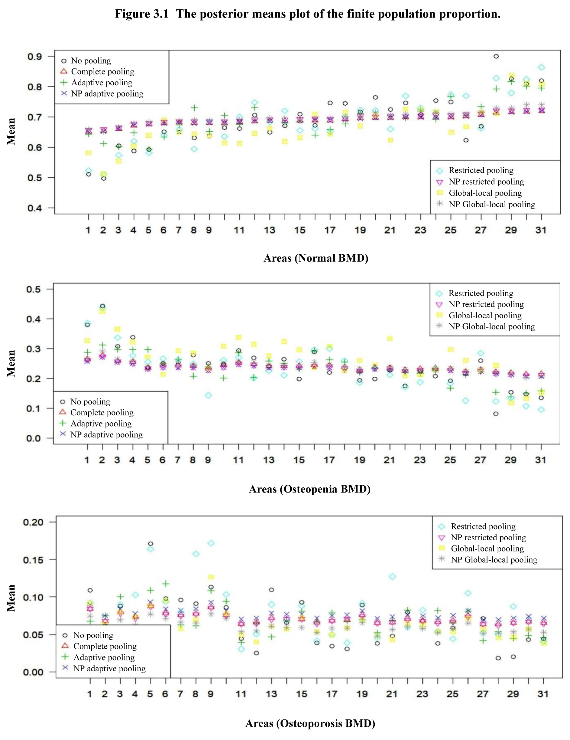
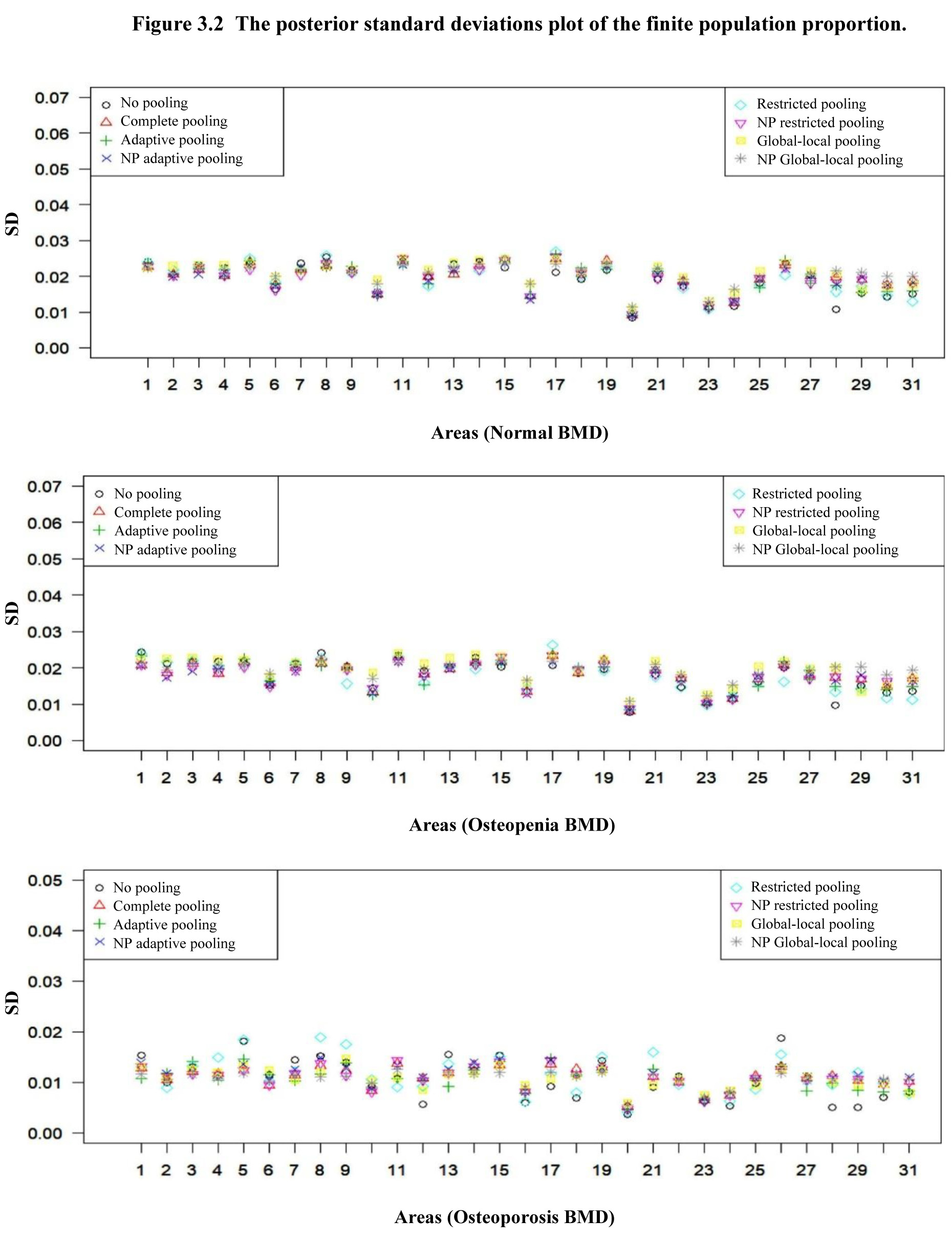
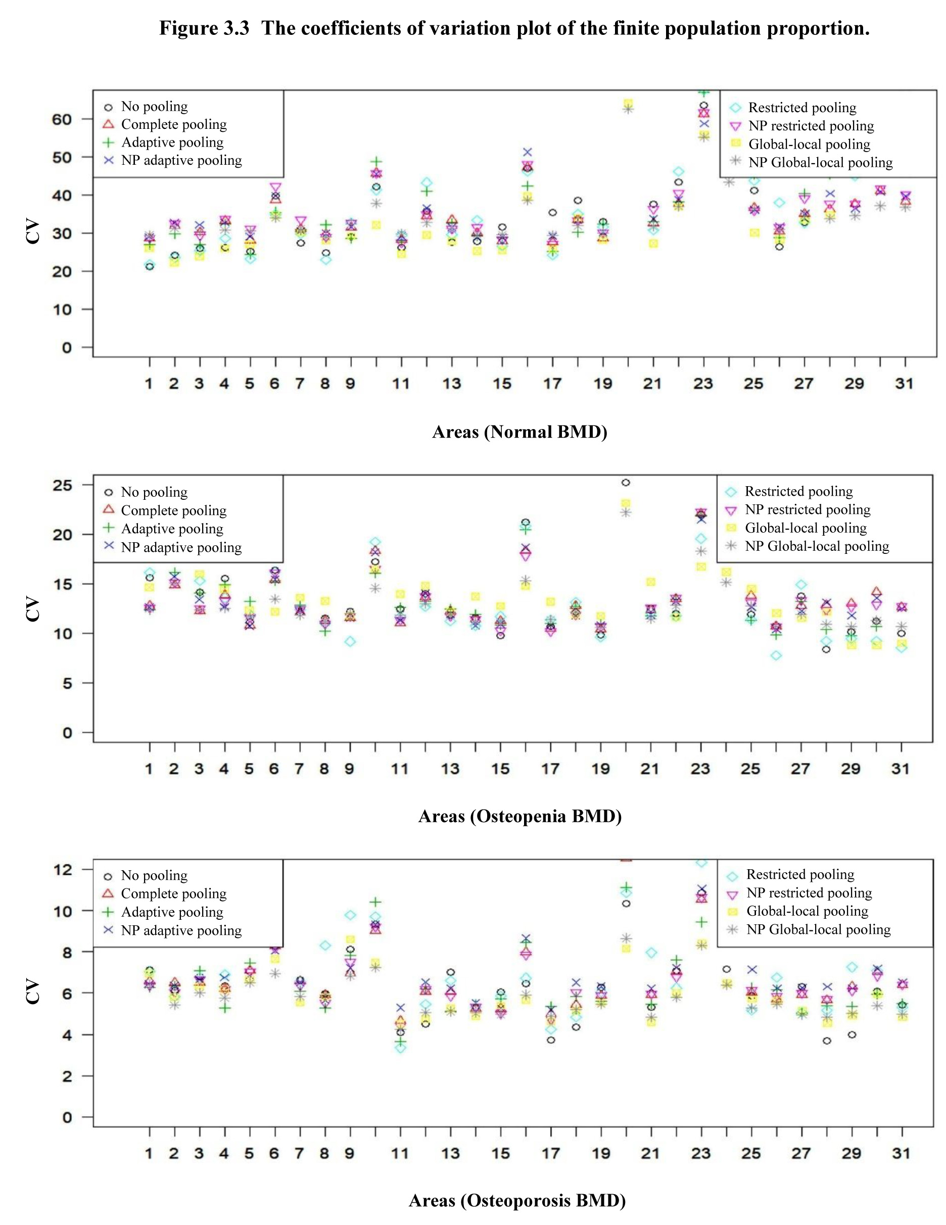
The posterior means, standard deviations (SD) and posterior coefficients of variation (CV) of the finite population proportions for the eight models can also be seen in Figure 3.1-3.3.

In Figure 3.1, the variation of PM for eight models is the largest in the normal BMD, which takes up the largest proportion. Especially, we can see that PMs of the nonparametric model are similar to that of the complete pooling model. During data analysis, we found one to three group index. Through this, we were able to discover that the BMD distribution is quite similar across the areas in NHANES III. Hence, all areas share their information with others to estimate the same hyperparameter. Thus, the nonparametric and complete pooling models give similar estimates. Therefore, pooling can solve problems associated with small area estimates when areas share similar traits. Furthermore, Figure 3.2 shows that the performance of the nonparametric models are good through the fact that the SD of the nonparametric models with many parameters are similar or smaller than that of the parametric models.

In addition, we can see the CV of the models by BMD status in Figure 3.3. In the case of CV, osteoporosis BMD shows the greatest difference between models. Also it can be seen that the CV of the nonparametric versions is relatively low compared to the parametric version, which is not different for each BMD status. Furthermore, it is very meaningful that the nonparametric version had a smaller CV than the models of the parametric version, even though it had infinite parameter space.

To estimate the parameters, we use a Gibbs sampler. Whereas the parameters with restricted parameter spaces are sampled using the grid method, the other parameters are sampled using the Metropolis-Hastings algorithm. We tune to get acceptance rate 30-70%. In the actual analysis, the acceptance rate of the algorithm is 34-49%. We compare the two measures in terms of the performance of each model. First, we calculate the deviance information criterion (DIC), a typical Bayesian model choice criterion, to compare the hierarchical Bayesian models. The DIC was proposed by Spiegelhalter et al. (2002), where a lower DIC value indicates better performance. Second, we evaluate the performance of the eight models by calculating the logarithmic conditional predictive ordinate (LCPO), which is a comparison method that uses cross validation. The average LCPO, proposed by Gneiting and Raftery (2007), is calculated as follows:

where ${{\displaystyle \text{C}\hat{\text{P}}\text{O}}}_i\mathrm{<mo>=</mo>}{\displaystyle {\sum }_{h\mathrm{<mo>=</mo>1}}^H{w}_{h}P(Y\mathrm{<mo>=</mo>}y|{\Omega }^{(h)})},$ $w_h\mathrm{<mo>=</mo>}{\displaystyle {\sum }_{h\mathrm{<mo>=</mo>1}}^{H}f(Y\mathrm{<mo>=</mo>}y|{\Omega }^{(h)})/f(Y\mathrm{<mo>=</mo>}y|{\Omega }^{(h)})},$ for $i\mathrm{<mo>=</mo>}\mathrm{1,}\dots ,I,$ and $P(Y=y|{\Omega }^{(h)})$ is the likelihood of a single observation of a given parameter ${\Omega }^{(h)},$ and $h\mathrm{<mo>=</mo>}\mathrm{1,}\dots ,H$ denotes the iterations from the MCMC result under the hierarchical Bayesian pooling model.

Table 3.3 shows the results of the two measures for each Bayesian pooling model. The model is considered to perform better as its estimated measures are smaller. The LCPO and DIC in parametric models are compared using the global-local pooling model, and LCPO and DIC have 12.707 and 4,984.56, respectively, implying the best performance. The restricted pooling model in Model 4 has an LCPO value of 12.886, showing the second-best performance after the global-local pooling model, but the DIC in the adaptive pooling model has a value of 4,998.90, which is lower than that in the restricted pooling model.

Another point to keep in mind is that the nonparametric version using the same pooling method shows similar values to those of the parametric method. In particular, although the nonparametric global-local pooling model has the greatest number of parameters to be estimated, its LCPO and DIC have values of 12.694 and 4,768.47, respectively, thereby indicating that it has the best performance among all the models. Additionally, in the restricted pooling model, the nonparametric model’s LCPO and DIC have values of 12.837 and 4,983.88, respectively, showing better performance than the parametric model. These results are identical in the LCPO scale of the adaptive pooling (i.e., base) model (LCPO (parametric vs nonparametric) = (13.411 vs 13.105)). This means the performance of the nonparametric version is very good for our data, even though the parameter space has infinite dimensions.

Table 3.4 illustrates the calculated statistical values to estimate the shrinkage of the model. To estimate shrinkage, we calculated the average and standard deviation of the absolute difference from the no shrinkage model for each BMD category. Let $\text{P}{\text{M}}_{ik},$ $i\mathrm{<mo>=</mo>}\mathrm{1,}\dots ,I,$ $k\mathrm{<mo>=</mo>}\mathrm{1,}\mathrm{2,}3$ denote the posterior mean of the finite population proportion for each cell in area $i.$ The average (ASE) and standard deviation (SDSE) of the shrinkage estimator are

$${\text{ASE}}_k\mathrm{<mo>=</mo>}\frac{1}{I}{\displaystyle \sum _{i\mathrm{<mo>=</mo>\; 1}}^I\frac{\left|{\text{PM}}_{ik}-{\text{PM}}_{0ik}\right|}{{\text{PM}}_{0ik}}\mathrm{,}I\mathrm{<mo>=</mo>}\mathrm{31,}}(3.3)$$

$${\text{SDSE}}_k\mathrm{<mo>=</mo>}\sqrt{\frac{1}{I-1}{\displaystyle \sum _{i\mathrm{<mo>=</mo>\; 1}}^I{\left(\frac{\left|{\text{PM}}_{ik}-{\text{PM}}_{0ik}\right|}{{\text{PM}}_{0ik}}-{\text{ASE}}_k\right)}^2}}\mathrm{,}(3.4)$$

where ${\text{PM}}_{0ik}$ is the posterior mean for the finite population proportion of Model 1, a no poooling model.

Based on this calculation, we show that the ASE and SDSE in the normal cell are the smallest in the global-local pooling model. Drawing from the data analysis, with the BMD data applied in this study, the number of groups of slice sampling is 1 to 3, and we can confirm that the data characteristics are identical for most regions. In the global-local model, however, it can be shown that the problem of overshrinkage induced by pooling is solved by looking at the smallest shrinkage degree. In addition, osteopenia cells and ostoporosis cells could confirm the tendency of low shrinkage relative to other models, and the SDSE in the global-local pooling model can be shown to be small. Meanwhile, in the case of nonparametric models, the group index had the highest number of 1 because of slice sampling; therefore, it could be suspected that data dependence was excessive in the no pooling model.

Also, Geweke’s test, autocorrelation plot and effective sample size (ESS) were applied for the diagnosis of the model, and they showed strongly mixing chains.

• Previous
• Article main page
• Next