Small area quantile estimation via spline regression and empirical likelihood

Section 6. Empirical application

• Previous
• Next

We now illustrate the proposed estimators based on the data set Survey of Labour and Income Dynamics (SLID) provided by Statistics Canada (2014) downloaded from University of British Columbia library data centre. The data contain 147 variables and 47,705 sample units. We are grateful to Statistics Canada for making the data set available, but we do not address the original goal of the survey here. Instead, we use it as a superpopulation to study the effectiveness of the proposed small area quantile estimator.

In this study, we singled out 9 of the 147 variables. They are ttin, gender, spouse, edu, age, yrx, tweek, jobdur and tpaid, standing respectively for: total income, gender, whether living with the spouse, the highest level of education, age, years of experience, number of weeks employed, education level, months of duration of current job and total hours paid at this job. After removing units containing missing values in these 9 variables as well as those with ttin $\le 0,$ we obtained a data set containing 28,302 sample units. The covariates power means at the population level are still calculated based on all available observations. We created 28 sub-populations (namely small areas) labeled as $4\left(k-1\right)+i\mathrm{,}$ $k\mathrm{<mo>=</mo>\; 1,}\mathrm{2,}\dots \mathrm{,}\mathrm{7,}$ $i\mathrm{<mo>=</mo>\; 1,}\mathrm{2,}\mathrm{3,}4$ based on gender-spouse-edu combinations. Here $k$ denotes education level and $i\mathrm{<mo>=</mo>\; 1,\; 2,\; 3,\; 4}$ denote male living with the spouse, female living with spouse, male not living with spouse and female not living with spouse respectively. The education levels are given as follows.

$$\begin{array}{ll}k\hfill & Highesteducationlevel\hfill \\ 1\hfill & \text{No more than 10 years elementary and secondary school}\hfill \\ 2\hfill & \text{11-13 years of elementary and secondary school }\left(\text{but did not graduate}\right)\hfill \\ 3\hfill & \text{Graduated high school}\hfill \\ 4\hfill & \text{Some university or non-university postsecondary with no certificate}\hfill \\ 5\hfill & \text{Non-university postsecondary or university certificate below Bachelor’s}\hfill \\ 6\hfill & \text{Bachelor’s degree}\hfill \\ 7\hfill & \text{University certificate above Bachelor’s}\hfill \end{array}$$

We regarded (ttin) as the response variable and fitted linear and additive non-parametric regressions with respect to other 5 variables. Based on the whole data, the adjusted R-square of the non-parametric fit is 0.482 which is much larger than 0.370 obtained by fitting the linear regression. This suggests that a non-parametric mixed model is a good choice. Figure 6.1 shows the fitted curves of log ttin with respect to these two covariates. Also, the R-square is as high as 0.483 even if the model includes only covariates age and tpaid and a random effect. These exploratory analyses prompt us to use only these two covariates in our simulation. We carried the simulation with sample sizes $n\mathrm{<mo>=</mo>\; 200};500$ and 1,000. To make sampling proportions in small areas close to their sizes, we let $n_i\mathrm{<mo>=</mo>}{a}_i+\mathrm{2,}i\mathrm{<mo>=</mo>\; 1,}\dots \mathrm{,}28$ with $a_i$ generated from the multinomial distribution with $p_i\mathrm{<mo>=</mo>}{N}_i/N.$

The simulated AMSE of 10 estimators based on 1,000 repetitions are reported in Table 6.1. We first notice that both our PEL estimators outperform the other estimators, in general, indicating the advantage of our non-parametric DRM based small area estimation technique. The PEL1 compared to PEL2 has the lower AMSE for 5%, 25%, and 50% quantiles, but slightly higher AMSE for 75% and 95% quantiles indicating the heteroscedasticity of data is not serious. Regardless the PEL estimators, we notice the LEL estimators outperform other estimators for 5% quantile, and have similar performance for other quantiles. Increasing the sample size reduces the AMSE of all estimators. Clearly, it is hard to estimate the 5% quantile with a good precision because the data are skewed toward the left so there are few observations for estimating the lower quantiles. Interestingly, LEL1 is not affected as much by the skewness. We feel that the kernel smoothing step (3.7) is helpful here. Without this smoothing step, LEL1 would perform much worse. Unreported simulations show that the ABIAS of all estimators decreases in general as the sample size increases and this is most apparent for DE.

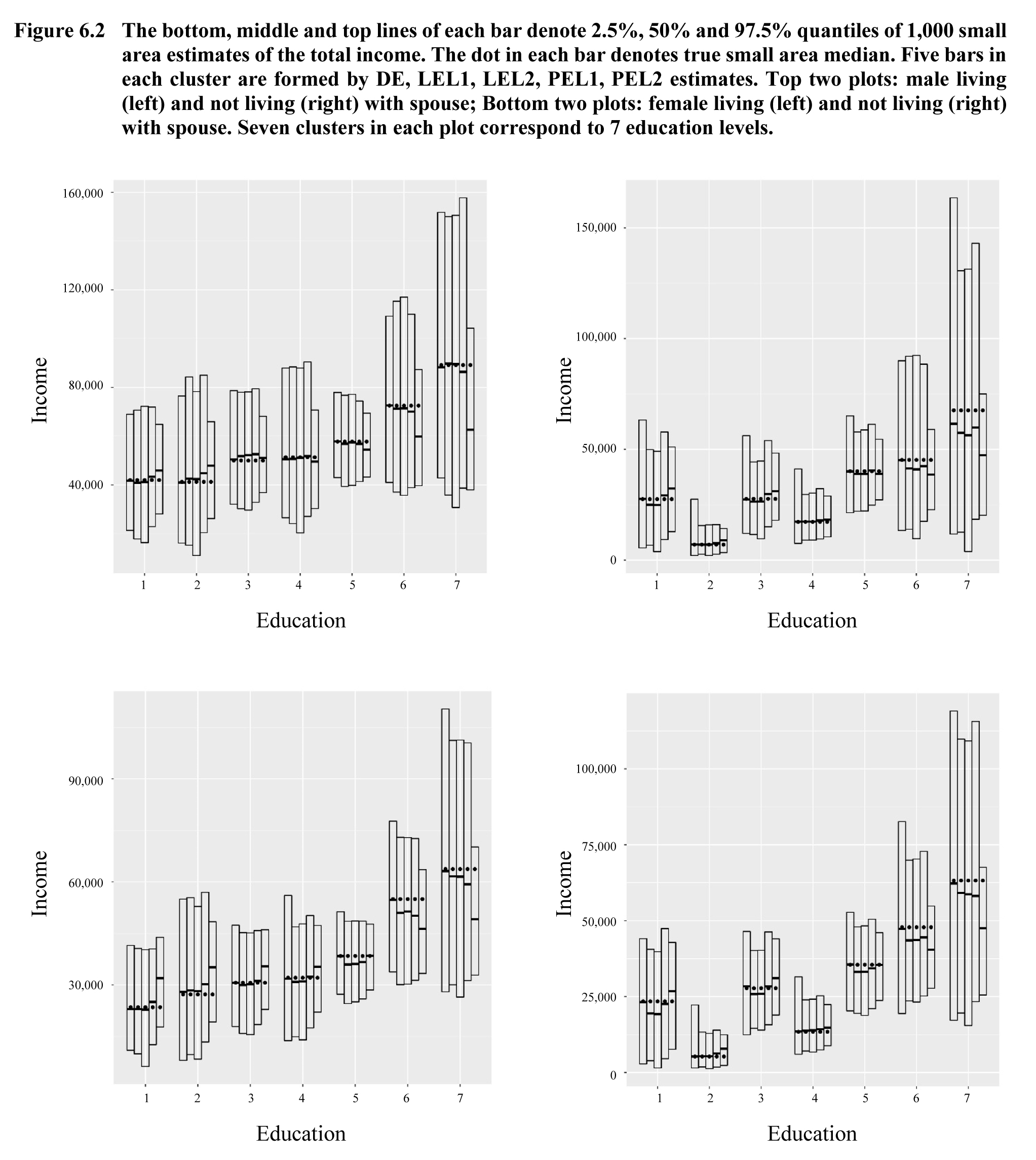
To check the performance of the proposed first estimator which using only covariate average information. In Figures 6.2, we depict the 2.5%, 50%, and 97.5% quantiles of 1,000 small area median estimates by the DE, LEL1, LEL2, PEL1, PEL2 with sample size $n\mathrm{<mo>=</mo>\; 200}$ with the true medians marked by dots. The y-axis is the total income and x-axis is the education level. It is seen that the PEL2 boxes are the shortest for most small areas.

Table 6.2 reports the bootstrap MSE estimates as well as the average ratios of bootstrap and simulated MSEs of the small area median estimators based on ${\widehat{F}}_i^{\left(a\right)}\left(u\right)$ and ${\widehat{F}}_i^{\left(b\right)}\left(u\right)$ with sample size $n\mathrm{<mo>=</mo>\; 200.}$ The number of simulation repetition is 500 with basis function $q_1\left(u\right)={\left(\mathrm{1,}u\right)}^{\prime }$ and $B\mathrm{<mo>=</mo>\; 100,}L\mathrm{<mo>=</mo>\; 100.}$ We can see the estimator ${\widehat{F}}_i^{\left(a\right)}\left(u\right)$ has higher MSE than ${\widehat{F}}_i^{\left(b\right)}\left(u\right),$ and most average ratios close to one.

• Previous
• Article main page
• Next