Measuring uncertainty associated with model-based small area estimators
Section 5. Simulation study

• Previous
• Next

In this section, we report the results of limited simulation studies on the design performance of the proposed composite MSE estimators. Section 5.1 gives results for the area level model, and the unit level model results are reported in Section 5.2.

5.1  Area-level model

Following the simulation set up used by Datta et al. (2011), we employ model (2.1) with $m=30$ areas, $z_i={\left(1,z_{i1}\right)}^{\prime }$ for $i=1,\dots ,m,$ where the covariate values $z_{i1},\dots ,z_{im}$ are generated independently from $N\left(-1,1\right)$ and held fixed over the simulation runs. Further, $\beta ={\left(1,1\right)}^{\prime },$ ${\sigma }_v^2=1$ and the sampling variance values are (2.0, 0.6, 0.5, 0.4, 0.2), with each different value of ${\psi }_i$ assigned to six consecutive areas. Noting that $v_i\sim N\left(0,1\right),$ we generate $\left\{{\theta }_i;i=1,\dots ,m\right\}$ from the linking model ${\theta }_i=z_i^{\prime }\beta +v_i$ and hold them fixed over the simulations to reflect the design-based approach conditioning on the area means ${\theta }_i.$ Then, $R=\text{100,000}$ simulated samples $\left\{{\widehat{\theta }}_i^{\left(r\right)}\text{}:i=1,\dots ,m\right\},$ $r=1,\dots ,R$ are generated from the sampling model ${\widehat{\theta }}_i={\theta }_i+e_i$ with the sampling error $e_i$ generated from $N\left(0,{\psi }_i\right)$ for specified sampling variance ${\psi }_i$ which is assumed fixed and known. We note that our simulation setup is not exactly design-based but it is “close enough” for the purposes of our study.

From the simulated data $\left\{\left({\widehat{\theta }}_i^{\left(r\right)}\text{},z_i\right):i=1,\dots ,m\right\}$ the EB estimates ${\widehat{\theta }}_i^{\text{EB}\left(r\right)}$ are computed and the MSE of ${\widehat{\theta }}_i^{\text{EB}}$ is approximated by

$${\text{MSE}}_i^{\text{EB}}=R^{-1}{\displaystyle \sum _{r=1}^R{\left({\widehat{\theta }}_i^{\text{EB}\left(r\right)}-{\theta }_i\right)}^2}\text{}.(5.1)$$

The MSE estimators for each simulated sample are computed and averaged over the 100,000 simulation runs. We denote the means of the MSE estimators over the simulations as ${\text{mse}}_i^{\text{EB}}\text{},$ ${\text{mse}}_{di}^{\text{EB}}\text{},$ ${\text{mod-mse}}_{di}^{\text{EB}}\text{},$ ${\text{mod-mse}}_{c1i}^{\text{EB}}$ and ${\text{mod-mse}}_{c2i}^{\text{EB}},$ corresponding to model, design unbiased, modified design unbiased, modified composite 1 and modified composite 2 MSE estimators, respectively. The relative bias (RB) of ${\text{mse}}_i^{\text{EB}}$ is given by

$${\text{RB}}_i^{\text{EB}}=\left({\text{mse}}_i^{\text{EB}}-{\text{MSE}}_i^{\mathrm{EB}}\right)/{\text{MSE}}_i^{\text{EB}}(5.2)$$

where ${\text{MSE}}_i^{\text{EB}}$ is given by (5.1). The absolute relative bias (ARB) is simply defined as ${\text{ARB}}_i^{\text{EB}}=\left|{\text{RB}}_i^{\text{EB}}\right|.$ The terms ${\text{ARB}}_{di}^{\text{EB}},$ ${\text{ARB}}_{di-\mathrm{mod}}^{\text{EB}},$ ${\text{ARB}}_{c1i-\mathrm{mod}}^{\text{EB}}$ and ${\text{ARB}}_{c2i-\mathrm{mod}}^{\text{EB}}$ are defined in a similar manner.

We also compute the relative root mean squared error (RRMSE) of the MSE estimators over the simulations. We denote those values as ${\text{RRMSE}}_i^{\text{EB}}\text{},$ ${\text{RRMSE}}_{di}^{\text{EB}}\text{},$ ${\text{RRMSE}}_{di-\mathrm{mod}}^{\text{EB}}\text{},$ ${\text{RRMSE}}_{c1i-\mathrm{mod}}^{\text{EB}}$ and ${\text{RRMSE}}_{c2i-\mathrm{mod}}^{\text{EB}}$ for the model, design unbiased, modified design unbiased, modified composite 1 and modified composite 2 MSE estimators, respectively. Here RRMSE of the model MSE estimator is defined as

$${\text{RRMSE}}_i^{\text{EB}}={\left\{R^{-1}{\displaystyle \sum _{r=1}^R{\left({\text{mse}}_i^{\text{EB}\left(r\right)}-{\text{MSE}}_i^{\text{EB}}\right)}^2}\right\}}^{1/2}/{\text{MSE}}_i^{\text{EB}}\text{}.(5.3)$$

The RRMSE of the other MSE estimators are similarly defined.

We first compare the average over all the areas of ${\text{mse}}_i^{\text{EB}}$ to the average over all areas of ${\text{mse}}_{di}^{\text{EB}}\text{}.$ We obtain 0.42 and 0.35 respectively, showing that the average of the model MSE estimator, 0.42, is close enough to the average of the design MSEs of the EB estimators, 0.35, confirming the theoretical result mentioned in Section 4.1. The theoretical result assumes known model parameters, while the simulation deals with the general case of unknown model parameters.

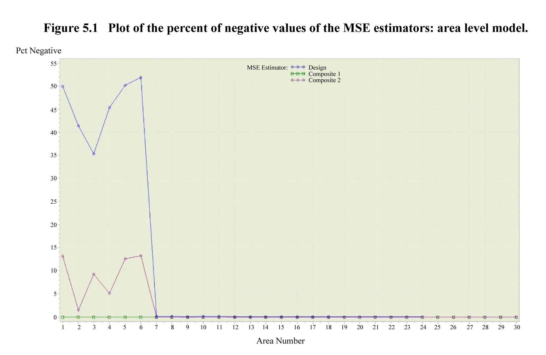
We next examine the probability of getting a negative value for the three MSE estimators: design unbiased, composite 1 and composite 2. Figure 5.1 shows the percentage of negative values over the simulations for each of the thirty areas. It is clear from Figure 5.1 that the probability of getting a negative value for the design unbiased MSE estimator can be as large as 50% for the first six areas (group 1) with much larger sampling variance relative to the remaining areas (group 2). On the other hand, it is negligible for the areas in group 2. The average probability over areas in group 1 is 45.67% compared to 0.03% in group 2. The probability of getting a negative value for the composite 1 MSE estimator is zero across all thirty areas, while the average probability for the composite 2 MSE estimator is 9.15% over areas in group 1 and zero over areas in group 2. The above results suggest that the composite 1 MSE estimator may not need modification even for areas with large sampling variances. Note that in the current simulation study the composite 1 and modified composite 1 MSE estimators are identical because no zero values were found for the composite 1 MSE estimator.

We now turn to the ARB of the MSE estimators. Figure 5.2 shows the ARB values across all the thirty areas for the MSE estimators: model, design unbiased, modified design unbiased, modified composite 1 and modified composite 2 MSE estimators. Table 5.1 gives the mean % design ARB values as well as the mean % design RRMSE over the areas in group 1 and group 2.

As expected, Figure 5.2 shows that the design unbiased estimator has zero ARB (except for simulation errors) across all areas. On the other hand, the modified design unbiased MSE estimator surprisingly exhibits a large ARB for the first six areas, with mean value of 93.49% but negligible for the remaining areas (0.38%). Model MSE estimator also exhibits large ARB for the first six areas with mean ARB of 51.66% that decreases to 25.76% for the remaining areas. On the other hand, the mean ARB for composite 1 MSE estimator is reduced to 34.08% for group 1 and small for group 2 (7.60%). The modified composite 2 MSE estimator that attaches more weight to the design unbiased MSE estimator reduces the mean ARB to 32.00% for group 1 and to 4.13% for group 2.

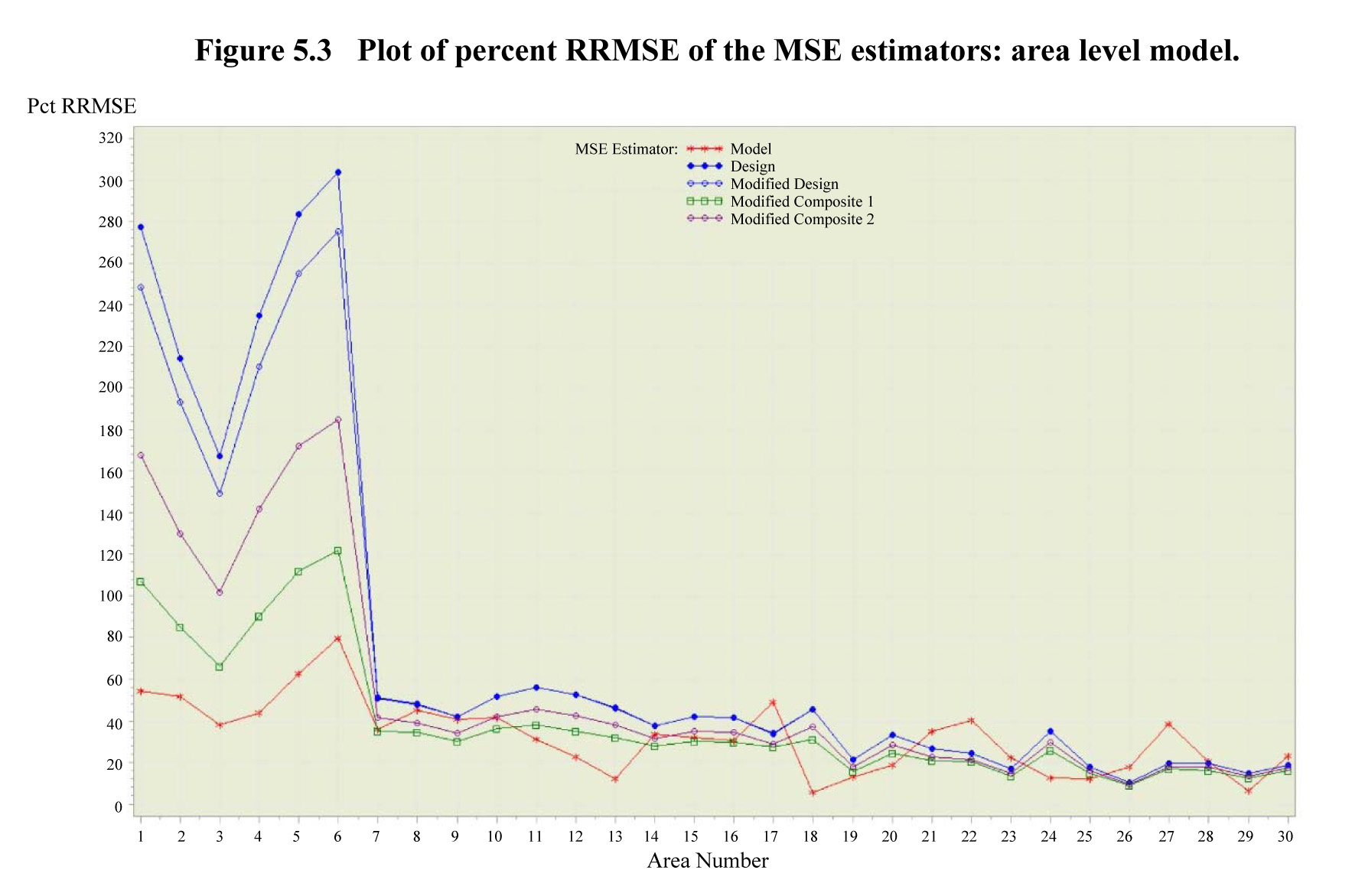
Figure 5.3 gives a plot of RRMSE of the MSE estimators across all the thirty areas and Table 5.1 reports the mean % RRMSE values for areas in group 1 and group 2. As expected, the design unbiased MSE estimator exhibits very large RRMSE for group 1 with mean value of 246.71%. The modified design unbiased MSE estimator is equally unstable for group 1 (mean RRMSE of 221.86%) in addition to exhibiting large ARB. Model MSE estimator exhibits the smallest RRMSE as expected with mean value of 54.98% for group 1 compared to 96.98% for composite 1 MSE estimator and 146.31% for modified composite 2 MSE estimator. On the other hand, for the areas in group 2 with smaller sampling variances, the mean RRMSE of the three MSE estimators is roughly the same: 24.70% for composite 1, 26.61% for model and 28.20% for modified composite 2 MSE estimators. The mean RRMSE for the design unbiased and modified design unbiased MSE estimators is only slightly larger for group 2 with values of 33.62% and 33.58% respectively.

Finally, we turn to confidence interval coverage rates for a nominal value of 95%. Normal theory coverage rates for the model MSE estimator are computed as

$$\text{CR}\left[\text{mse}\left({\widehat{\theta }}_i^{\text{EB}}\right)\right]=R^{-1}{\displaystyle \sum _{r=1}^{R}I\left[{\widehat{\theta }}_i^{\text{EB}\left(r\right)}-\text{1}\text{.96}{\left({\text{mse}}_i^{\text{EB}\left(r\right)}\right)}^{1/2}\le {\theta }_i\le {\widehat{\theta }}_i^{\text{EB}\left(r\right)}+\text{1}\text{.96}{\left({\text{mse}}_i^{\text{EB}\left(r\right)}\right)}^{1/2}\right]}(5.4)$$

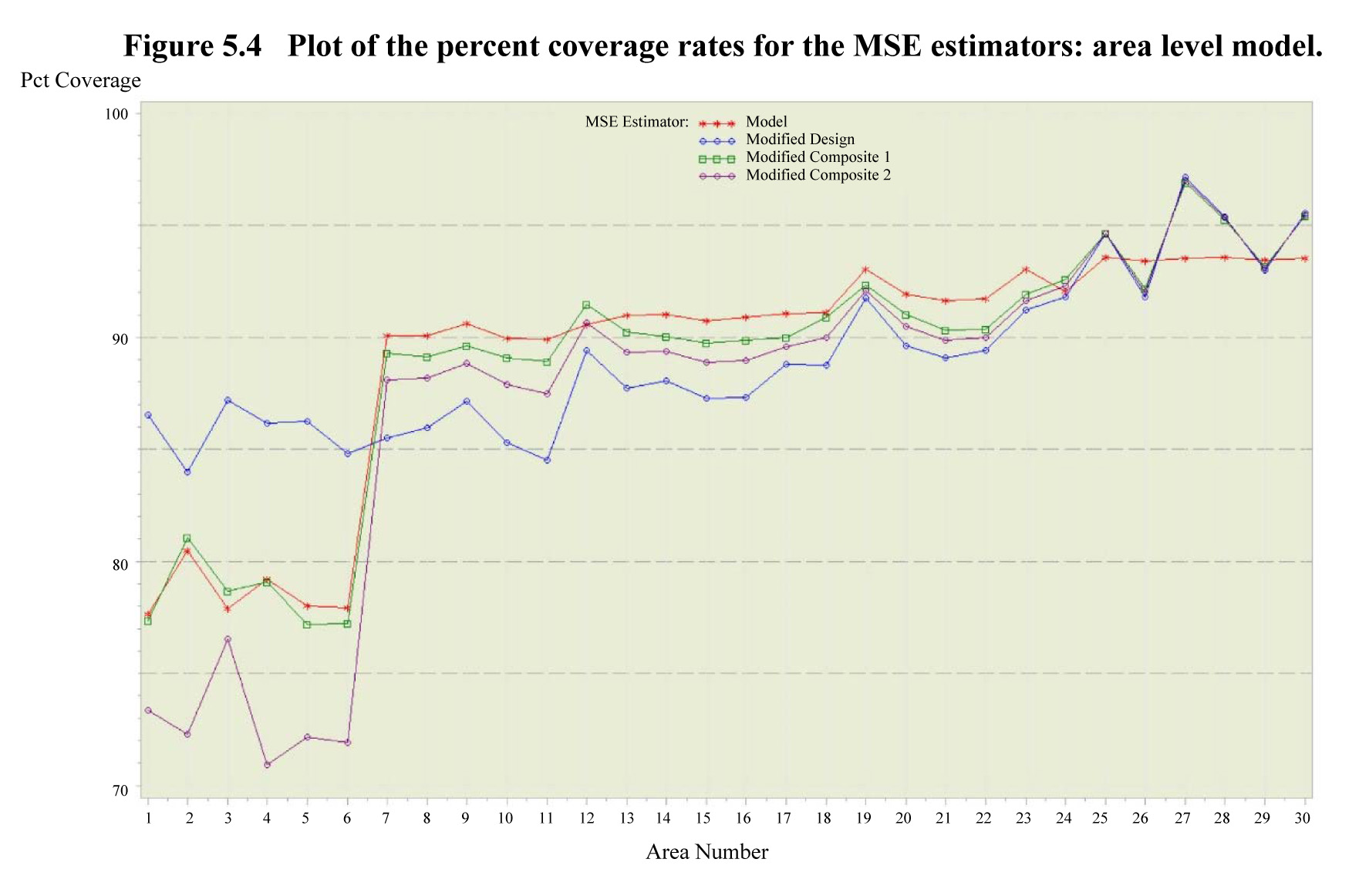
where $I[·]$ is an indicator function with value 1 if ${\theta }_i$ is in the calculated interval and 0 otherwise. Coverage rates for the other MSE estimators are similarly defined. Figure 5.4 is a plot of the percent coverage rates for the MSE estimators. The curve associated with the design-unbiased MSE estimator is not included in the plot because it is not possible to calculate the confidence interval coverage rate due to negative MSE estimates for some simulation runs. Discarding these simulation runs and calculating the intervals from the remaining runs can distort the coverage rate.

The plot shows serious undercoverage for areas in group 1 with large sampling variance. In particular, the mean coverage rate for model, modified composite 1 and modified composite 2 are 68.53%, 78.43% and 72.87% respectively, whereas the modified design MSE estimator show some improvement: 85.82%. On the other hand, for the areas in group 2 with smaller sampling variances, the mean coverage rate increases to 91.73%, 91.74%, 90.89% and 89.85% for the model, modified composite 1, modified composite 2 and the modified design MSE estimators, respectively. Figure 5.4 suggests that the coverage rates for the model and modified composite MSE estimators are comparable across all areas with the areas in group 1 exhibiting serious undercoverage because of small sample sizes or large sampling variances in those areas.

5.2  Unit-level model

In this section, we report some results of a limited simulation study on the design performance of four MSE estimators under a simple unit-level mean model given by

$$y_{ij}=\beta +v_i+e_{ij},j=1,\dots ,N_i;i=1,\dots ,m(5.5)$$

where the area random effects $v_i\stackrel{\text{iid}}{{\displaystyle \sim }}N\left(0,{\sigma }_v^2\right)$ are independent of the unit errors $e_{ij}\stackrel{\text{iid}}{{\displaystyle \sim }}N\left(0,{\sigma }_e^2\right).$ The MSE estimators studied include the model MSE estimator $\text{mse}\left({\widehat{\overline{Y}}}_i^{\text{EB}}\right),$ of the EB estimator ${\widehat{\overline{Y}}}_i^{\text{EB}}$ (Rao and Molina, 2015, Section 7.2.3), the plug-in design-based MSE estimator ${\text{mse}}_d^{*}\left({\widehat{\overline{Y}}}_i^{\text{EB}}\right)$ obtained from (4.9) by replacing the model parameters $\beta ,$ ${\sigma }_v^2$ and ${\sigma }_e^2$ by their REML estimators, the composite MSE estimator given by (4.10), and a “conditional” MSE estimator, ${\text{mse}}_{\text{CH}}\left({\widehat{\overline{Y}}}_i^{\text{EB}}\right),$ proposed by Chambers, Chandra and Tzavidis (2001, Section 2.2.2).

For the design-based simulation, we use $m=30$ small areas and first generate the area population sizes $N_i,$ from a Uniform distribution $U\left[\text{443,}\text{542}\right]$ and hold them fixed over simulation runs, following Chambers et al. (2011). We generate two fixed finite populations $\left\{y_{ij},j=1,\dots ,N_i;i=1,\dots ,m\right\}$ from the mean model (5.5) for specified mean parameter $\beta =500$ and variance parameters ${\sigma }_v^2=\text{10}\text{.40},$ ${\sigma }_e^2=\text{94}\text{.09}$ for the first finite population (denoted Population A) and $\beta =500,$ ${\sigma }_v^2=\text{40}\text{.32},$ ${\sigma }_e^2=\text{94}\text{.09}$ for the second finite population (denoted Population B). Note that the variance ratio $\delta ={\sigma }_v^2/{\sigma }_e^2$ is equal to 0.11 for Population A and is smaller than the value 0.43 for Population B. We then draw stratified simple random samples $\left\{y_{ij},j=1,\dots ,n_i;i=1,\dots ,30\right\}$ without replacement, from each finite population, treating each area as a stratum, where the area sample sizes are chosen to be equal: either $n_i=5$ or $n_i=20.$ In all, we draw $S=\text{10,000}$ stratified simple random samples and compute the MSE estimates from each sample. Independently, we also draw $R=\text{30,000}$ stratified random samples and compute the EB estimates from each sample. The MSE of the EB estimator for each area is approximated along the lines of (5.1) using the 30,000 simulation runs. Using a large number of simulation runs, $R=\text{30,000},$ the true MSE of the EB estimator is accurately approximated by the empirical MSE. On the other hand, a smaller number of simulation runs, such as $S=\text{10,000},$ is used for studying the performance of the four MSE estimators to reduce computations. This two-step simulation setup is often used for the unit level model (see e.g., González-Manteiga, Lombardia, Molina, Morales and Santamaria, 2008). Typically, calculating the MSE is much faster than calculating the RB and RRMSE of several MSE estimators, particularly bootstrap MSE estimators.

Using the simulated MSE estimates and the simulated MSE of the EB, we compute the relative bias (RB), the absolute relative bias (ARB) and the relative root mean square error (RRMSE) of the MSE estimators along the lines of (5.2) and (5.3). In the case of Population A and area sample size 5, the plug-in design-based MSE estimator leads to underestimation across all areas, with RB ranging from -87.0% to -18.1%. This underestimation is due to ignoring the variability in the parameter estimates. On the other hand, the model MSE estimator generally overestimates the design MSE with RB ranging from -66.4% to 150.1%. As a result, the composite MSE estimator reduces the underestimation caused by the plug-in design-based MSE estimator: RB ranging from -55.0% to 115.4%. The conditional MSE estimator overestimates the design MSE consistently with RB ranging from 31.7% to 316.1%. Performance of the MSE estimators in terms of RB improves as the ratio $\delta$ increases to 0.43 or the area sample size increases to 20.

Table 5.2 reports the median and mean ARB values for the two populations and the two sample sizes. It shows that the composite MSE estimator performs better than the other MSE estimators for Population A and area sample size 5, with median and mean ARB equal to 53%. On the other hand, the conditional MSE estimator exhibits large median ARB equal to 208% and mean ARB equal to 191%. Median and mean ARB values for all the MSE estimators decrease as the ratio $\delta$ increases to 0.43 or the area sample size increases to 20.

Table 5.3 reports the median and mean % design RRMSE values for the two populations and the two sample sizes. It shows that the model MSE estimator and the composite MSE estimator perform better than the other MSE estimators, especially for Population A and area sample size 5. In the latter case, the plug-in design-based MSE estimator and the conditional MSE estimator exhibit large median and mean RRMSE values: approximately 400% versus 110% for the model MSE estimator and the composite MSE estimator. Performance of all the MSE estimators improves in terms of RRMSE as the ratio $\delta$ increases or the area sample size increases. In the case of population B and area sample size 20, model MSE estimator exhibits the smallest median and mean RRMSE: approximately 10% versus 30% for the other MSE estimators.

• Previous
• Article main page
• Next