A cautionary note on Clark Winsorization Section 4. Detection regionsA cautionary note on Clark Winsorization Section 4. Detection regions

• Previous
• Next

We examine the range of influential values that Clark Winsorization designates as influential, called the detection region, under three scenarios. One scenario has a single high influential value present in the sample. In the other two scenarios, the sample contains two high influential values.

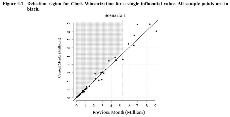
Figures 4.1 and 4.2 use grids of unweighted data to illustrate the detection regions for the application of the Clark Winsorization algorithm on a single sample from a simulated MRTS industry with low volatility, a monthly revenue of $2.5 billion and a sample size of 147. In these figures, each $\left(x,y\right)$ point on the grid represents a possible influential value where $x$ represents the unweighted value for the previous month and $y$ represents the current month’s unweighted value. Since the weights for the same business rarely change from month-to-month, the scatterplots of weighted values are similar and therefore are not shown. We use sampling weights for the points on the grid and do not modify the weights in our simulation. All the points on a vertical line have the same weight with the sample weights lower for units that have higher values of sales. The detection regions are constructed by inserting each pair of $\left(x,y\right)$ coordinates from the grid into the sample and then running the Clark Winsorization algorithm with the parameter settings described in Section 3 to see if the weighted $y$ value in the inserted pair is designated as influential.

4.1 Results for one influential value

In this section, we illustrate the effect on the detection region of a sample containing a single influential value, hereafter referred to as Scenario 1. In Figure 4.1, the unweighted sample observations used to form the detection regions are shown in black with the $x-$axis representing the previous month’s value and the $y-$axis representing the current month. The robust least median of squares regression line used in the prediction model has been included for reference. For the given sample, a single observation that falls in the light gray hashed region (detection region) is flagged as influential and adjusted by the Clark Winsorization method. The broken vertical line marks the largest sampled observation with a weight greater than one; that is, all observations to the right of this asymptote are guaranteed to have a weight of one.

The close proximity of the lower boundary line of the detection region to the regression line reflects the trimming done by the method to minimize the MSE by lowering the variance at the cost of introducing a small bias. Therefore, several non-influential cases in this detection region will be trimmed slightly nonetheless. We observed this phenomenon repeatedly in several other (different) empirical data sets.

4.2 Results for two influential values

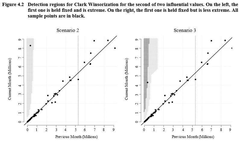
Now we turn to investigating the detection region when the sample contains two induced high influential values. Our approach holds one induced observation at a fixed value and weight in the sample and allows the second induced observation to vary in value with its corresponding weight, permitting the identification of the detection region for the second observation, conditional on the first. This approach allows us to assess whether the procedure is subject to masking which occurs when a large value prevents the identification of other extreme values. We consider two scenarios for the fixed value. In Scenario 2, the contribution of the fixed influential value to the estimate of total sales is 667 million higher than the previous month. In Scenario 3, the fixed influential value is less severe since its contribution is 334 million higher, half of the increase in Scenario 2.

The graph on the left in Figure 4.2 presents the detection region (light gray area) under Scenario 2. Here, the fixed (unweighted) value is 350,000 in the previous month and 8.2 million in the current month with a weight of 85. Regardless of where the second observation was placed throughout the graph, the fixed observation was always designated as influential. Notice that the observations that would have been falsely designated as influential and slightly trimmed in Scenario 1 (see Figure 4.1) would not have been changed in this scenario. Here, the detection region is restricted to identifying only similar severe observations, which are supposed to be atypical.

The dramatic difference in the relative sizes of the detection regions between Scenario 1 and Scenario 2 could indicate that this procedure $–$ as applied $–$ is vulnerable to masking. Masking occurs when one influential value causes a failure to identify the presence of another (Barnett and Lewis 1994). We explore this possibility in Scenario 3, halving the unweighted value of the fixed influential value in the current month (now 4.1 million instead of 8.2 million) while allowing the weight to retain the same value of 85. The graph on the right in Figure 4.2 shows two different shaded regions: a light grey area where both the fixed influential value and the second (variable) value can be detected, and a dark gray region to the left of the light gray region where the algorithm detects the variable value as influential but misses the fixed value. Adjustments in the light gray area reduce both the bias and the MSE. In the dark gray area, the adjustment reduces the MSE, but may not reduce the bias substantially. The white area to the right of the light gray region shows where only the fixed influential value is identified. However, the white area contains large observations with small weights so these observations are not representing much more than themselves, and consequently adjustments in this range have small impact on the bias.

This preliminary exploration validates our concern about the potential for masking. One approach that may alleviate masking when a stationary series has a high level of noise is to average $L$ over several previous months as suggested in Chambers et al. (2000). The sampling design may be a factor. The graph on the left in Figure 2.1 shows that the weights decline rapidly as the unweighted observations increase for observations between 0 and 1 million. In this range, the weight of the unit has more impact than its observed value on the size of its weighted residual used in calculating the $k^{*}.$ A relatively small change in the variable value may trigger a much larger change in its weighted residual and cause the $k^{*}$ to change, which affects the number of influential values detected. The weights used in this example reflect the weights used in the MRTS for the industry and were not constructed artificially to create an illustration for the Clark Winsorization methodology.

• Previous
• Next