
Analytical Studies Branch Research Paper Series
Environmentally Adjusted Multifactor Productivity Growth for the Canadian Manufacturing Sector

Archived Content
Information identified as archived is provided for reference, research or recordkeeping purposes. It is not subject to the Government of Canada Web Standards and has not been altered or updated since it was archived. Please "contact us" to request a format other than those available.
by Wulong Gu, Jakir HussainNote 1 and Michael Willox
Economic Analysis Division,
Analytical Studies Branch,
Statistics Canada
Acknowledgements
The authors would like to thank Bob Gibson of Statistics Canada, Nouri Najjar of the University of Western Ontario, and Dylan Morgan of Environment and Climate Change Canada for their invaluable contributions to building a world-class dataset. They are also grateful to Chris O’Donnell, Lynda Khalaf and the other participants of the June 2018 Carleton University Productivity Mini-workshop for their invaluable feedback as well as to Samuel Gamtessa of the University of Regina for his insightful comments. The authors are responsible for any errors or omissions.
Abstract
The need to measure both the desirable outputs (goods and services) and the undesirable outputs (emissions of greenhouse gases [GHGs] and criteria air contaminants [CACs]) from economic activity is becoming increasingly important as economic performance and environmental performance become ever more intertwined. Standard measures of multifactor productivity (MFP) growth provide insights into rising standards of living and the performance of economies, but they may be misleading if only desirable outputs are considered. This study presents estimates of environmentally adjusted multifactor productivity (EAMFP) growth using a new comprehensive database. This database contains information on GHG and CAC emissions, as well as on the production activities of Canadian manufacturers. Overall, the results indicate that EAMFP growth was higher than MFP growth, largely reflecting declines in the undesirable output emissions intensity, in the manufacturing sector from 2004 to 2012.
Keywords: Environment, productivity, output distance function, shadow price
Executive summary
Seminal reports relating the economy and the environment, such as those by Stern (2008) and Stiglitz, Sen and Fitoussi (2009), have helped reveal the extent to which economic activity and the environment are inextricably linked to each other. An important implication of this literature is that standard measures of economic activity examined in isolation from the environment are potentially misleading. Productivity, defined most simply as the efficiency with which inputs are transformed into outputs, can be particularly sensitive to refinements in how it is measured. The benchmark measure of productivity used in this study is multifactor productivity (MFP), which typically measures a single output (real gross output) relative to inputs used in production (physical capital, labour and intermediate inputs, which include energy, materials and services). If MFP grows over time, it may be the result of improvements in efficiency, technology and the quality of the products made as well as changes in the scale of production (Baldwin et al. 2014; Syverson 2011). Estimates of environmentally adjusted multifactor productivity (EAMFP) growth presented in this study incorporate the production of undesirable outputs that are jointly produced with desirable output. These undesirable outputs consist of emissions of greenhouse gases (GHGs), which induce climate change, and criteria air contaminants (CACs), which reduce air quality.
The findings of this study indicate that accounting for undesirable outputs from the Canadian manufacturing sector leads to a lower level of EAMFP than of MFP. The difference between MFP and EAMFP reflects the fact that total output is calculated differently for the two productivity measures. In the case of MFP, total output includes only desirable output. Total output for EAMFP also includes the undesirable outputs that are jointly produced with the desirable output. Undesirable outputs, because they are unwanted, are subtracted from desirable output, making the total output associated with EAMFP lower than that associated with MFP. Since both productivity measures are calculated as their respective total outputs relative to the same inputs, the level of EAMFP is lower than that of MFP, except in the trivial case where no undesirable outputs are produced.
However, the growth of MFP and EAMFP is a different story. In a simple case where the quantity of inputs does not change over time but desirable output increases, MFP grows. In addition, if undesirable outputs decline, EAMFP growth will be higher than MFP growth. Put another way, if the quantity of GHG and CAC emissions relative to the quantity of goods and services produced (i.e., undesirable output intensity) declines, EAMFP will grow faster than MFP. The general decline in the undesirable output intensity of Canadian manufacturers was the primary reason for EAMFP growth being stronger than MFP growth from 2004 to 2012.
The calculation of EAMFP growth requires that prices of different types of GHGs and CACs be estimated. The prices of undesirable outputs reflect the trade-off between the intensity with which desirable and undesirable outputs are produced with a given amount of inputs. As undesirable output intensity declines, the cost of reducing it more tends to increase, which is reflected in higher absolute prices for undesirable outputs.
1 Introduction
The realization that the environment and the economy are becoming ever more interwoven is not new. The Brundtland Commission (WCED 1987, p. 37) noted that “Environment and development are not separate challenges; they are inexorably linked…in a complex system of cause and effect.” More recent studies, including those by Stern (2008) and Stiglitz, Sen and Fitoussi (2009), have reinvigorated the debate and shifted the discourse toward how the interaction between the environment and the economy can be better measured. To that end, a number of recent studies from the Organisation for Economic Co-operation and Development (OECD) estimate a measure of productivity growth that accounts for the generation of a small set of greenhouse gases (GHGs) and criteria air contaminants (CACs)—broadly referred to as undesirable outputs—from economic activity. These studies include those by Brandt, Schreyer and Zipperer (2014); Dang and Mourougane (2014); and Cárdenas Rodríguez, Haščič and Souchier (2016). Specifically, each of these three OECD studies adopt commonly used approaches rooted in the use of output distance functions to derive a shadow price for each of the undesirable outputs. The estimated shadow prices then allow environmentally adjusted multifactor productivity (EAMFP) growth to be calculated in a growth accounting framework.
A similar approach is used in this study, with some important differences. First, the OECD studies all use real gross domestic product (GDP) as a measure of desirable output, whereas this study focuses on real gross output, a more inclusive measure of desirable output, although estimates using real GDP are also provided for comparison. Second, the data used in the OECD studies are at the aggregate, total economy level to facilitate international comparisons, while the data used in this study are at the business establishment level for the manufacturing sector only. Using microdata allows one to analyse the trade-off between jointly produced desirable and undesirable outputs that result from individual establishments’ production decisions. On the other hand, using data at a national level means the trade-off between desirable and undesirable outputs not only within and between establishments as well as the trade-off between industries and regions may not be captured directly.
The remainder of this paper proceeds as follows: Section 2 presents the methodology, Section 3 provides a detailed description of the linked dataset used, Section 4 reviews some key empirical findings, Section 5 notes areas for future work and Section 6 concludes the paper. Two appendices provide additional information on EAMFP growth and shadow prices for select manufacturing subsectors and a comparison of estimates for the manufacturing sector using real gross output and real GDP.
2 Methodology
In this study, a Shephard output distance function is estimated to derive shadow prices for undesirable outputs. The shadow prices are then used to derive EAMFP growth, using a growth accounting framework with undesirable outputs similar to that used by Brandt, Schreyer and Zipperer (2014). EAMFP growth is measured as the difference between the growth in the combined desirable and undesirable outputs and the growth in factor inputs.
A key piece of information needed to estimate EAMFP growth is the seldom-observed prices of undesirable outputs. These are a crucial element for creating weights that, along with the quantities of undesirable outputs, are necessary for growth accounting. The prices of undesirable outputs can be represented by shadow prices, which are the optimal private costs of reducing undesirable outputs for individual business establishments. These should not be taken as the optimal social costs, which would also account for the impact of undesirable outputs on public institutions and infrastructure, social justice, and the health and income of individuals. Shadow prices of undesirable outputs—the opportunity cost of abating undesirable outputs in the form of reduced desirable output—are found to vary widely across different types of undesirable outputs. Low shadow prices (in absolute terms) may be observed because the production of undesirable outputs is large relative to that of desirable output or because the trade-off between changes in desirable and undesirable outputs is low, as expressed by an undesirable output elasticity. In either situation, shadow prices often increase when regulations are introduced, regulations are strengthened or compliance with existing regulations improves (Cárdenas Rodríguez, Haščič and Souchier 2016).
2.1 The estimation of shadow prices of undesirable outputs
The methodology used in two recent OECD studies, Brandt, Schreyer and Zipperer (2014) and Dang and Mourougane (2014), to estimate the shadow prices of undesirable outputs is adopted in this study. In their approach, the shadow prices of undesirable outputs are derived parametrically using an output distance function. All producers are assumed to operate on the production possibility frontier, implying that all producers are perfectly technically efficient and that producers maximize profits by taking into account the costs of reducing undesirable outputs. Similar to Brandt, Schreyer and Zipperer (2014), this study uses estimated shadow prices in a growth accounting framework to derive estimates of EAMFP growth for the Canadian manufacturing sector. This study extends Brandt, Schreyer and Zipperer (2014) and Dang and Mourougane (2014) by using establishment-level microdata to account for the establishment heterogeneity.
The remainder of this section presents the methodology for estimating shadow prices of undesirable outputs as well as the growth accounting framework with undesirable outputs used to estimate EAMFP growth.
2.2 A framework for estimating environmentally adjusted multifactor productivity growth
The growth accounting framework begins with the measurement of growth of desirable output () expressed as the change in the logarithm of desirable output and divided by the change in time, , as shown on the left-hand side of Equation (1).
(1)
Desirable output growth, , can be separated into the sum of contributions from growth in the factors of production, namely labour (), capital () and intermediate inputs (), as well as multifactor productivity (MFP) growth, which represents changes in efficiency and advances in technology.Note 2 The contributions from labour, capital and intermediate inputs are multiplied by their respective weights, represented by their nominal shares in desirable output. Nominal shares are expressed as for labour (where is the wage rate and is the price of desirable output), for capital (where is the rental rate of capital) and for intermediate inputs (where is the price of intermediate inputs). If perfect competition is assumed, these shares can be regarded as the marginal products of labour, capital and intermediate inputs, respectively. They also represent the elasticity of desirable output with respect to factor inputs.
Decomposing desirable output growth into contributions from input growth and MFP growth allows MFP growth to be estimated residually by rearranging Equation (1), since information on desirable output, labour, capital and intermediate inputs, as well as their prices, is readily available in the KLEMS (capital, labour, energy, materials, services) database:Note 3
(2)
Note that factor inputs are aggregated so that .
This approach can be adjusted to account for the effect of economic activity on the environment by representing the value of total output as the combined value of desirable and undesirable outputs, expressed as , where is the price of an individual undesirable output to be estimated and is the observed quantity of undesirable output measured in tonnes. The value of total nominal output is lower than that of nominal desirable output, since the price of undesirable output, , is typically negative, reflecting the fact that it is an unwanted by-product of the production process.
The contribution of changes in desirable and undesirable output to total output growth can be expressed as follows:
(3)
where total output is defined as ; its growth, , is equal to the nominal share-weighted growth of desirable and undesirable outputs.
Replacing the output growth term in Equation (2) with the right-hand side of Equation (3) produces an expression that measures the growth of EAMFP:
(4)
Equation (4) can be simplified by rearranging terms
(5)
where is undesirable output’s share of total output. Unfortunately, the prices of undesirable outputs are not observed and, therefore, need to be estimated. To do so, the approach used by Brandt, Schreyer and Zipperer (2014) and Dang and Mourougane (2014) are followed. They begin by defining a production technology for an output set, as follows:
(6)
which states that the production technology can produce desirable output and undesirable output using inputs . The production technology is assumed to satisfy the axioms found in Färe and Primont (1995).
The production function in Equation (6) can be equivalently expressed as an output distance functionNote 4 defined by Shephard (1970) to estimate the marginal rate of transformation (MRT) between desirable and undesirable outputs. This relates the shadow price of undesirable output to that of desirable output. The output distance function is the inverse of the proportion by which the production of total output could be increased while remaining within the feasible production set with a given set of inputs (Coelli and Perelman 1996).Note 5 It is expressed as
(7)
The value of the output distance function ranges from 0 to 1. If total output is located on the production function, which can be represented graphically at point in Figure 1, then . However, if total output is located on the interior of the production set at point , then . The distance function can be thought of as a ray from the origin, where output at implies , whereas at , . The distance function is homogeneous of degree 1 in desirable output and undesirable outputs: non-decreasing in desirable output and non-increasing in undesirable output and factor inputs. The distance function also exhibits weak disposability, meaning that an establishment can reduce undesirable output only by simultaneously reducing desirable output (Coelli and Perelman 1996, 1999).

Description for Figure 1
The title of Figure 1 is “A production possibility frontier with desirable and undesirable outputs.”
The figure shows a straight line representing the vertical axis labelled “ ” that extends up from the origin. The label represents desirable output.
It also shows a straight line representing the horizontal axis labelled “ ” that extends to the right from the origin. The label represents undesirable output.
An arched line forming a semi-circle labelled “Production possibility frontier” lies on the horizontal axis. The production possibility frontier starts at the origin on the left.
A straight line extends from the origin between the and axes and underneath the production possibility frontier until it intersects the production possibility frontier at a point labelled “ ”. The line passes through a point labelled “ ”, about midway between the origin and . The point represents the actual amount of total output produced and represents the level of output produced if production were perfectly technically efficient.
Another straight line labelled “Slope” is tangent to the production function at point . It represents the marginal rate of transformation. The label for the fourth line also includes a mathematical function, . It indicates that the slope is equal to the marginal rate of transformation of desirable and undesirable outputs ( ) and is also equal to the negative value of the price of desirable output ( ) divided by the price of undesirable output ( ).
The slope of at point represents the MRT between outputs and , which is equivalent to the ratio of the prices of desirable output to the price of an individual undesirable output. It is calculated as
(8)
Note that whether production occurs at or at , reflecting changes in efficiency in production, the is not affected. Consequently, assuming perfect efficiency, as is typically done in a growth accounting framework for estimating MFP growth, does not impact how shadow prices for undesirable outputs are derived.
The objective then is to estimate the output distance function, taking partial derivatives with respect to desirable and undesirable output (Aiken and Pasurka 2003). Unfortunately, the output distance function, like the price of undesirable outputs, is not directly observable. However, if the output distance function is assumed to be homogeneous of degree 1 in desirable and undesirable outputs (Färe and Grosskopf 1990; Färe et al. 1993), it can be rewritten as
(9)
Taking logs, rearranging terms and adding to reflect the panel structure of the data give the following expression:
(10)
The output distance function can be represented in a Cobb–Douglas form where the logged distance function on the right-hand side of Equation (10) represents inefficiency, which is assumed to be zero in a standard growth accounting framework. After dividing through by time and including establishment-fixed effects, , and a random noise term, , Equation 10 takes the following form:
(11)
where and
Rearranging terms to separate desirable and undesirable outputs produces an equation that can be estimated as
(12)
where and are equal to and , respectively.
Time , measured in years, is also included to capture technical change as a time trend, and captures establishment fixed effects.
As noted by Brandt, Schreyer and Zipperer (2014), it would be desirable to take advantage of a more flexible functional form, such as a translog function. In particular, they express concerns that the Cobb–Douglas form is not well suited for an output distance function because it violates the condition that the distance function be convex in outputs. While Coelli and Perelman (1996) also acknowledge such concerns, they indicate that the problem is not particularly serious when the primary interest is in obtaining technical measures such as efficiency estimates. More practically, the Cobb–Douglas form is favoured over the translog function because, similar to the findings of Brandt, Schreyer and Zipperer (2014), results from a translog function are almost universally statistically insignificant and frequently produce positive shadow prices for undesirable outputs, which makes little economic sense. These results occur whether the translog function is specified with capital, labour and intermediate inputs separately or with a single aggregate input (as expressed in Equation [12]), and with a single undesirable output or various combinations of multiple undesirable outputs.
Following Brandt, Schreyer and Zipperer (2014), the undesirable output shadow price is derived as the solution to the revenue-over-unit-of-output maximization problemNote 6 that relates the distance function at the frontier of efficiency to the elasticity of desirable output with respect to an undesirable output, , in Equation (12).Note 7 The shadow price can then be expressed as
(13)
With shadow prices of undesirable outputs in hand, EAMFP growth rates from Equation (5) can be estimated for comparison with official MFP estimates.
3 Data
Estimating EAMFP was made possible due to the development of the linked NPRI-GHGRP-ASML dataset. The NPRI-GHGRP-ASML dataset is the most comprehensive source of information on undesirable outputs and production available for Canada’s manufacturing sector. It includes plant-level emissions, abatement activities, sales, employment, and production expenses of many of the largest producers of undesirable outputs among Canadian manufacturers from 2001 to 2012. The dataset combines information from three sources: the National Pollutant Release Inventory (NPRI), the Greenhouse Gas Reporting Program (GHGRP), and the Annual Survey of Manufactures and Logging (ASML) making research related to the interaction of economic activity and the environment at the establishment level possible.
Environment and Climate Change Canada (ECCC) collects pollution and GHG emissions data annually under the authority of the Canadian Environmental Protection Act, 1999. Under this act, the GHGRP and the NPRI were established. All industrial establishments (not just manufacturers) that meet specified criteria and release thresholds must report annually to ECCC on their emissions of various GHGs (for the GHGRP) and of over 300 pollutants (for the NPRI) according to ECCC (2015).
Each of the datasets includes information for different levels of business organizations. The ASML is an establishment-based survey, while the NPRI and the GHGRP are facility-based. A facility is potentially a smaller unit of observation than an establishment. As a result, some establishments in the ASML include one or more facilities in the NPRI and GHGRP. When an establishment in the ASML is associated with multiple facilities, the releases of pollutants were aggregated to the establishment level.
Coverage of facilities differs between the NPRI and GHGRP largely because of differences in the specified inclusion criteria for the NPRI and release thresholds for both the NPRI and GHGRP. All facilities that emit GHGs in excess of the minimum reporting threshold must report to the GHGRP, although any facility may voluntarily report its emissions. The minimum reporting threshold from 2004 to 2008 was 100,000 tonnes of GHGs in carbon dioxide equivalent units. After 2008, the threshold fell to 50,000 tonnes. To ensure that changes in GHG emission thresholds did not skew the results, only establishments that emitted 100,000 tonnes or more were included in the analysis for the entire nine-year period. This reduces the total number of observations by 27% to 29% for each of the four types of GHG emissions examined.
The NPRI inclusion requirements are based on both the amount emitted of a given pollutant and the facility’s size (measured by employment). In general, large facilities that emit more than a minimum emission threshold are required to report their emissions. The minimum emission threshold varies by pollutant. For certain substances, a minimum concentration threshold may be used instead of a minimum release threshold. Facilities that do not meet the inclusion requirements may still voluntarily report to the NPRI. The following are the inclusion criteria used in the NPRI:
- Plants employing more than 10 workers (full-time equivalent) must report to the NPRI on each pollutant they emit above the minimum release threshold (or the minimum concentration threshold).
- Plants that employ fewer than 10 workers (full-time equivalent) and operate a device that uses a fossil fuel input (e.g., boiler or generator) must report to the NPRI on each of the CACs emitted above the minimum release threshold.
- Plants that employ fewer than 10 workers (full-time equivalent) and do not operate a device that uses a fossil fuel input are not required to report to the NPRI.
Any plant that emits less than the minimum release threshold or the minimum concentration threshold for a given pollutant is not required to report on that pollutant to the NPRI.
In 2006, 15 additional volatile organic compounds (VOCs) were added to the list of pollutants that establishments were required to report on if they emitted more than specific thresholds. However, these additional pollutants did not contribute substantially to total releases of VOCs in manufacturing, because many firms voluntarily reported on these pollutants before 2006. This explains why releases of these 15 VOCs increased only 2.4% from 2005 to 2006. This increase represents 0.1% of total releases of VOCs, compared with VOC levels in 2005. As a result, the inclusion of additional VOCs in 2006 had no discernible impact on the shadow price of VOCs or its related EAMFP growth.
The ASML is an annual survey of Canada’s manufacturers and logging. It is intended to cover all manufacturing establishments, together with associated head offices, sales offices and auxiliary units that have been classified as manufacturing industries. Detailed information collected includes principal industrial statistics (such as shipments, employment, salaries and wages, cost of materials and supplies used, cost of purchased fuel and electricity used, inventories, and goods purchased for resale) and commodity data, including shipments or consumption of particular products.
Ideally, establishment-level data for prices of GDP, gross output, capital, labour and intermediate inputs would be used. However, such detailed price information is rarely available. As a result, industry-level price data for three-digit North American Industry Classification System codes from Statistics Canada’s annual multifactor productivity accounts (also known as the KLEMS database), Table 36-10-0217-01 (Statistics Canada n.d.) (formerly CANSIM table 383-0032), were used.
4 Empirical results for the Canadian manufacturing sector
Results for the Canadian manufacturing sector are presented for the years 2004 to 2012. Emissions of undesirable outputs were divided into two major categories, GHGs and CACs . Results are provided for total GHGs, as well as for three major subcomponents: carbon dioxide (CO2), methane (CH4) and nitrous oxide (N2O). Results for CACs include total particulate matter (TPM), particulate matter equal to or less than 10 microns in diameter (PM10), particulate matter equal to or less than 2.5 microns in diameter (PM2.5), sulphur dioxide (SO2), nitrogen oxides (NOx), volatile organic compounds (VOCs), carbon monoxide (CO) and ammonia (NH3).Note 8 See Table 1 for a summary of abbreviations.
| Abbreviation | Name |
|---|---|
| GHG | Greenhouse gasTable 1 Note 1 |
| CO2 | Carbon dioxide |
| N2O | Nitrous oxide |
| CH4 | Methane |
| CACs | Criteria air contaminants |
| CO | Carbon monoxide |
| NOx | Nitrogen oxides |
| SO2 | Sulphur dioxide |
| TPM | Total particulate matter |
| PM10 | Particulate matter equal to or less than 10 microns in diameter |
| PM2.5 | Particulate matter equal to or less than 2.5 microns in diameter |
| VOC | Volatile organic compound |
| NH3 | Ammonia |
|
|
4.1 Emissions of undesirable outputs
Total emissions of GHGs in the manufacturing sector—largely consisting of three of the most important gases, CO2, CH4 and N2O, in carbon dioxide equivalent measures—were lower in 2012 than in 2004. This decline is consistent to some degree with the secular decline in manufacturing since the earlier 2000s. The modest rebound in emissions of GHGs after the financial crisis and recession of 2008/2009 mostly reflects higher emissions of CO2 and CH4. In contrast, N2O continued to decline (Chart 1).

Data table for Chart 1
| 2004 | 2005 | 2006 | 2007 | 2008 | 2009 | 2010 | 2011 | 2012 | |
|---|---|---|---|---|---|---|---|---|---|
| index (2004 = 100) | |||||||||
| Greenhouse gases | 100.0 | 85.2 | 87.7 | 90.4 | 84.1 | 65.0 | 74.1 | 80.8 | 88.3 |
| Carbon dioxide | 100.0 | 86.8 | 93.5 | 96.3 | 87.2 | 69.9 | 80.9 | 88.0 | 95.8 |
| Nitrous oxide | 100.0 | 85.5 | 47.4 | 55.0 | 78.9 | 29.3 | 13.7 | 13.6 | 11.2 |
| Methane | 100.0 | 78.2 | 50.9 | 44.9 | 42.4 | 49.1 | 56.2 | 62.8 | 54.5 |
|
Note: All releases of greenhouse gases are in carbon-dioxide-equivalent measures. Source: Statistics Canada, authors’ calculations based on linked data from the National Pollutant Release Inventory, the Greenhouse Gas Reporting Program, the Annual Survey of Manufactures and Logging, and Statistics Canada Table 36-10-0217-01. |
|||||||||
Other GHGs not shown in Chart 1 include hydrofluorocarbons, sulphur hexafluoride and perfluorocarbons. Information on sulphur hexafluoride and perfluorocarbons cannot be released for confidentiality reasons, while the quantities of hydrofluorocarbons released were relatively low, contributing negligible amounts to total GHG emissions.
Similar to the trends for GHGs, emissions of CACs in the manufacturing sector generally trended downward from 2004 to the 2008/2009 recession, before rebounding modestly until 2012. Chart 2 shows trends in the emissions of eight CACs: TPM, PM10, PM2.5, SO2, NOx, VOCs, CO and NH3.

Data table for Chart 2
| 2004 | 2005 | 2006 | 2007 | 2008 | 2009 | 2010 | 2011 | 2012 | |
|---|---|---|---|---|---|---|---|---|---|
| index (2004 = 100) | |||||||||
| Carbon monoxide | 100.0 | 92.1 | 92.5 | 98.1 | 97.3 | 61.5 | 99.0 | 81.1 | 95.2 |
| Nitrogen oxides | 100.0 | 93.2 | 82.9 | 83.8 | 80.9 | 71.5 | 75.8 | 74.3 | 84.4 |
| Sulphur dioxide | 100.0 | 47.8 | 88.2 | 71.4 | 68.4 | 48.0 | 63.9 | 71.0 | 67.3 |
| Total particulate matter | 100.0 | 87.9 | 88.4 | 91.0 | 77.4 | 63.9 | 70.5 | 80.1 | 84.8 |
| Particulate matter ≤ 10 microns in diameter | 100.0 | 91.7 | 92.6 | 92.0 | 80.3 | 65.4 | 69.4 | 77.6 | 86.3 |
| Particulate matter ≤ 2.5 microns in diameter | 100.0 | 93.4 | 93.7 | 85.6 | 79.6 | 62.1 | 67.1 | 72.9 | 79.5 |
| Volatile organic compounds | 100.0 | 83.7 | 75.4 | 78.6 | 70.1 | 71.3 | 78.1 | 79.0 | 81.8 |
| Ammonia | 100.0 | 100.9 | 118.3 | 135.3 | 131.0 | 115.6 | 114.1 | 114.1 | 124.9 |
|
Source: Statistics Canada, authors’ calculations based on linked data from the National Pollutant Release Inventory, the Greenhouse Gas Reporting Program, the Annual Survey of Manufactures and Logging, and Statistics Canada Table 36-10-0217-01. |
|||||||||
Changes in CAC emissions over the nine-year period reveal a general downward trend, with the exception of NH3. It is also worth noting that, from 2007 to 2009, the compound annual rate of decline for all eight undesirable outputs was on average 13.3%, nearly 13 times faster than for the entire period. This suggests that the recession of 2008/2009 was strongly associated with emissions levels.
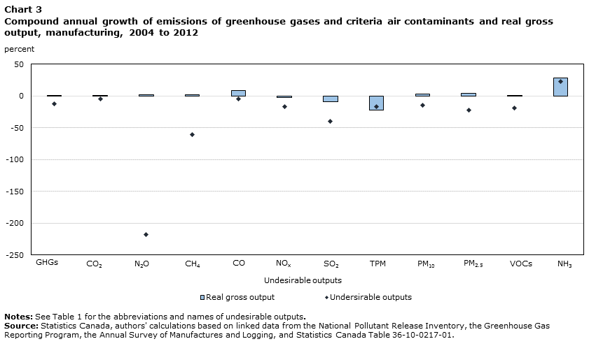
Growth rates of desirable and undesirable outputs are reported in Chart 3. The growth rates of desirable output differ for each undesirable output, because an establishment that produces CO2, for example, may produce only some or none of the other undesirable outputs. Therefore, the calculation of real gross output growth related to CO2 includes only establishments that report CO2 emissions. From 2004 to 2012, the growth rates of all undesirable outputs examined—GHGs and CACs —were lower than the growth rates of desirable output (real gross output), with the exception of TPM. In other words, the largest emitters of undesirable outputs in the Canadian manufacturing sector saw their undesirable output intensity decline, on average, for most GHGs and CACs .
Data table for Chart 3
| Undesirable outputs | Real gross output | Undersirable outputs |
|---|---|---|
| percent | ||
| GHGs | 0.5 | -12.5 |
| CO2 | 0.5 | -4.3 |
| N2O | 2.1 | -218.6 |
| CH4 | 1.6 | -60.8 |
| CO | 8.0 | -5.0 |
| NOx | -2.9 | -17.1 |
| SO2 | -9.4 | -39.6 |
| TPM | -22.4 | -16.5 |
| PM10 | 3.4 | -14.7 |
| PM2.5 | 4.2 | -22.9 |
| VOCs | 0.1 | -19.5 |
| NH3 | 28.0 | 22.2 |
|
Notes: See Table 1 for the abbreviations and names of undesirable outputs. Source: Statistics Canada, authors' calculations based on linked data from the National Pollutant Release Inventory, the Greenhouse Gas Reporting Program, the Annual Survey of Manufactures and Logging, and Statistics Canada Table 36-10-0217-01. |
||
4.2 Estimation results for undesirable outputs
Equation (12) was estimated as a panel fixed-effect regression. Because of the large number of undesirable outputs and because sample sizes for many undesirable outputs and manufacturing subsectors can reduce the robustness of estimates, the approach taken in this paper follows that of Brandt, Schreyer and Zipperer (2014) and Dang and Mourougane (2014). In this approach, coefficients for undesirable outputs are estimated individually in separate regressions. Table 2 shows the coefficients for, undesirable output growth, technical change and related calculations for each undesirable output resulting from separate estimations.
| Undesirable outputs | Undesirable output growth | Technical change | F-test for constant returns to scale |
Observations | Undesirable output shadow price | ||
|---|---|---|---|---|---|---|---|
| coefficient | standard error | coefficient | standard error | p-value | number | $ 2012/tonne | |
| GHGs | 0.233 | 0.040 | 0.002 | 0.004 | 0.000 | 548 | -389.87 |
| CO2 | 0.260 | 0.042 | 0.002 | 0.004 | 0.000 | 549 | -453.05 |
| N2O | 0.004 | 0.012 | 0.002 | 0.004 | 0.104 | 468 | -1,002.38 |
| CH4 | 0.015 | 0.010 | 0.002 | 0.004 | 0.061 | 475 | -3,611.29 |
| CO | 0.047 | 0.012 | 0.002 | 0.003 | 0.000 | 1,375 | -19,950.05 |
| NOx | 0.022 | 0.014 | 0.002 | 0.002 | 0.000 | 1,510 | -34,874.77 |
| SO2 | 0.005 | 0.008 | 0.003 | 0.003 | 0.000 | 913 | -1,489.13 |
| TPM | 0.027 | 0.012 | 0.002 | 0.003 | 0.000 | 1,405 | -69,665.77 |
| PM10 | 0.036 | 0.009 | 0.001 | 0.002 | 0.000 | 1,936 | -229,573.26 |
| PM2.5 | 0.025 | 0.008 | 0.001 | 0.002 | 0.000 | 1,934 | -260,041.91 |
| VOCs | 0.062 | 0.012 | 0.003 | 0.003 | 0.000 | 1,446 | -211,975.14 |
| NH3 | 0.017 | 0.012 | 0.004 | 0.005 | 0.231 | 461 | -91,779.94 |
|
Note: See Table 1 for the abbreviations and names of the undesirable outputs. Source: Statistics Canada, authors’ calculations based on linked data from the National Pollutant Release Inventory, the Greenhouse Gas Reporting Program, the Annual Survey of Manufactures and Logging, and Statistics Canada Table 36-10-0217-01. |
|||||||
For consistency with a growth accounting framework, like that of Brandt, Schreyer and Zipperer (2014), a basic assumption required for estimating undesirable output shadow prices using an output distance function is constant returns to scale in the three factor inputs, capital, labour and intermediate inputs. Based on the results of the F-test given in Table 2, the null hypothesis that the production technology exhibits constant returns to scale was not rejected for N2O, CH4 and NH3. However, it was clearly rejected for all of the remaining undesirable outputs. For most emissions, estimating an unconstrained output distance function would be more appropriate. However, doing so would violate the assumption of homogeneity of degree 1 of the output distance function, which could in turn lead to distorted estimates of shadow prices for these undesirable outputs, as well as the corresponding environmental adjustments to MFP growth. This issue is likely related in part to using establishment-level data as opposed to highly aggregated country-level data for which constant returns to scale have not been as problematic in most OECD studies.Note 9
4.3 Estimated shadow prices for undesirable outputs
The price associated with an undesirable output is typically negative; it represents the cost to establishments of reducing the undesirable output in terms of reduced desirable output. Most of the estimated shadow prices of undesirable outputs trend downward over time. Shadow prices decrease (increase in absolute terms) over the whole sample period (Chart 4). This is because the GHG and CAC intensity of production in manufacturing has generally declined over the nine-year period. The elasticity of undesirable outputs is estimated as time-invariant coefficients—these estimates therefore contribute to changes in undesirable output prices. Of the undesirable outputs examined, those that were statistically significant at a 5% level of significance for a two-tailed test included total GHGs, CO2, CO, TPM, PM10, PM2.5 and VOCs. The shaded area around each estimated shadow price in Chart 4 indicates the distribution around the mean shadow price for a 5% level of significance.

Data table for Chart 4-1
| 2004 | 2005 | 2006 | 2007 | 2008 | 2009 | 2010 | 2011 | 2012 | |
|---|---|---|---|---|---|---|---|---|---|
| 2012 dollars | |||||||||
| GHGs | |||||||||
| Shadow price | -298 | -336 | -317 | -341 | -357 | -310 | -350 | -381 | -390 |
| 95% CI | |||||||||
| Upper bound | -397 | -448 | -422 | -454 | -476 | -414 | -467 | -508 | -520 |
| Lower bound | -198 | -224 | -211 | -227 | -238 | -207 | -233 | -254 | -260 |
| CO2 | |||||||||
| Shadow price | -376 | -416 | -375 | -403 | -434 | -364 | -404 | -441 | -453 |
| 95% CI | |||||||||
| Upper bound | -495 | -548 | -494 | -532 | -572 | -479 | -533 | -581 | -597 |
| Lower bound | -256 | -283 | -256 | -275 | -296 | -248 | -276 | -301 | -309 |
| N2O | |||||||||
| Shadow price | -96 | -107 | -189 | -180 | -123 | -223 | -614 | -743 | -1,002 |
| 95% CI | |||||||||
| Upper bound | -632 | -703 | -1,243 | -1,188 | -812 | -1,468 | -4,044 | -4,895 | -6,600 |
| Lower bound | 440 | 490 | 865 | 827 | 565 | 1,022 | 2,815 | 3,408 | 4,595 |
| CH4 | |||||||||
| Shadow price | -1,684 | -2,045 | -3,083 | -3,874 | -3,994 | -2,316 | -2,608 | -2,791 | -3,611 |
| 95% CI | |||||||||
| Upper bound | -3,781 | -4,592 | -6,923 | -8,700 | -8,970 | -5,201 | -5,857 | -6,268 | -8,110 |
| Lower bound | 414 | 502 | 757 | 952 | 981 | 569 | 641 | 686 | 887 |
| CO | |||||||||
| Shadow price | -15,241 | -17,573 | -17,824 | -16,583 | -16,266 | -20,231 | -14,998 | -22,383 | -19,950 |
| 95% CI | |||||||||
| Upper bound | -22,576 | -26,031 | -26,403 | -24,564 | -24,095 | -29,968 | -22,217 | -33,156 | -29,552 |
| Lower bound | -7,905 | -9,115 | -9,245 | -8,601 | -8,437 | -10,493 | -7,779 | -11,610 | -10,348 |
| TPM | |||||||||
| Shadow price | -64,258 | -64,066 | -70,235 | -67,637 | -71,607 | -66,155 | -74,263 | -73,202 | -69,666 |
| 95% CI | |||||||||
| Upper bound | -118,480 | -118,127 | -129,501 | -124,711 | -132,031 | -121,978 | -136,929 | -134,972 | -128,452 |
| Lower bound | -10,035 | -10,005 | -10,969 | -10,563 | -11,183 | -10,331 | -11,598 | -11,432 | -10,880 |
|
Notes: See Table 1 for the abbreviations and names of the undesirable outputs. CI: confidence interval. Source: Statistics Canada, authors' calculations based on linked data from the National Pollutant Release Inventory, the Greenhouse Gas Reporting Program, the Annual Survey of Manufactures and Statistics Canada Table 36-10-0217-01. |
|||||||||

Data table for Chart 4-2
| 2004 | 2005 | 2006 | 2007 | 2008 | 2009 | 2010 | 2011 | 2012 | |
|---|---|---|---|---|---|---|---|---|---|
| 2012 dollars | |||||||||
| NOx | |||||||||
| Shadow price | -26,346 | -27,432 | -31,505 | -31,045 | -32,031 | -28,007 | -32,191 | -37,133 | -34,875 |
| 95% CI | |||||||||
| Upper bound | -58,983 | -61,413 | -70,531 | -69,504 | -71,711 | -62,702 | -72,068 | -83,132 | -78,076 |
| Lower bound | 6,291 | 6,550 | 7,522 | 7,413 | 7,648 | 6,687 | 7,686 | 8,866 | 8,327 |
| SO2 | |||||||||
| Shadow price | -957 | -1,009 | -1,149 | -1,416 | -1,342 | -1,457 | -1,323 | -1,379 | -1,489 |
| 95% CI | |||||||||
| Upper bound | -3,948 | -4,159 | -4,740 | -5,841 | -5,535 | -6,010 | -5,454 | -5,687 | -6,141 |
| Lower bound | 2,033 | 2,142 | 2,441 | 3,008 | 2,851 | 3,095 | 2,809 | 2,929 | 3,163 |
| PM10 | |||||||||
| Shadow price | -166,624 | -161,499 | -183,156 | -181,066 | -202,733 | -209,353 | -232,688 | -240,498 | -229,573 |
| 95% CI | |||||||||
| Upper bound | -251,212 | -243,485 | -276,137 | -272,986 | -305,652 | -315,633 | -350,813 | -362,588 | -346,118 |
| Lower bound | -82,036 | -79,513 | -90,176 | -89,146 | -99,814 | -103,074 | -114,562 | -118,407 | -113,029 |
| PM2.5 | |||||||||
| Shadow price | -172,475 | -159,836 | -186,911 | -204,654 | -214,649 | -229,755 | -252,354 | -268,527 | -260,042 |
| 95% CI | |||||||||
| Upper bound | -278,918 | -258,478 | -302,262 | -330,956 | -347,120 | -371,549 | -408,095 | -434,249 | -420,527 |
| Lower bound | -66,032 | -61,193 | -71,559 | -78,352 | -82,179 | -87,962 | -96,614 | -102,806 | -99,557 |
| VOCs | |||||||||
| Shadow price | -151,589 | -171,828 | -207,372 | -188,159 | -204,819 | -160,907 | -169,888 | -202,622 | -211,975 |
| 95% CI | |||||||||
| Upper bound | -210,696 | -238,825 | -288,229 | -261,525 | -284,681 | -223,647 | -236,130 | -281,627 | -294,627 |
| Lower bound | -92,483 | -104,830 | -126,515 | -114,793 | -124,957 | -98,167 | -103,646 | -123,617 | -129,323 |
| NH3 | |||||||||
| Shadow price | -75,414 | -79,026 | -73,939 | -66,351 | -70,845 | -65,490 | -84,582 | -87,441 | -91,780 |
| 95% CI | |||||||||
| Upper bound | -180,384 | -189,023 | -176,856 | -158,705 | -169,455 | -156,646 | -202,313 | -209,151 | -219,530 |
| Lower bound | 29,556 | 30,971 | 28,978 | 26,004 | 27,765 | 25,666 | 33,149 | 34,269 | 35,970 |
|
Notes: See Table 1 for the abbreviations and names of the undesirable outputs. CI: confidence interval. Source: Statistics Canada, authors' calculations based on linked data from the National Pollutant Release Inventory, the Greenhouse Gas Reporting Program, the Annual Survey of Manufactures and Statistics Canada Table 36-10-0217-01. |
|||||||||
The relatively high absolute prices of PM2.5, PM10 and VOCs reflect the high cost associated with reducing emissions of these undesirable outputs. In contrast, the results suggest that CO2 would be much less costly to reduce. Emissions of N2O had a relatively low cost in 2004, but as they fell sharply over time, abatement costs rose commensurately.
4.4 Comparison of estimates of shadow prices among studies
Estimates of shadow prices can vary widely among studies because of differences in methodology, scope (industry or total economy), data sources and estimation methods.
| Study | Scope | Methodology |
|---|---|---|
| Appendix A, Table A.1 | Manufacturing, Canada, real gross output | Parametric estimation of an output distance function and growth accounting |
| Appendix A, Table A.1 | Manufacturing, Canada, real GDP | Parametric estimation of an output distance function and growth accounting |
| Brandt, Schreyer and Zipperer (2014)Table 3-1 Note 1 | Total economy, Canada, real GDP | Parametric estimation of an output distance function and growth accounting |
| Dang and Mourougane (2014) | Total economy, Canada, real GDP | Parametric estimation of an output distance function |
| Cárdenas Rodríguez, Haščič and Souchier (2016) | Total economy, Canada, real GDP | Parametric estimation of a random coefficient model and growth accounting |
Sources: Statistics Canada (Appendix A, Table A.1); N. Brandt, P. Schreyer and V. Zipperer, 2014, Productivity Measurement with Natural Capital and Bad Outputs; T. Dang and A. Mourougane, 2014, Estimating Shadow Prices of Pollution in OECD Economies; and Cárdenas Rodríguez, I. Haščič, and M. Souchier, 2016, Environmentally Adjusted Multifactor Productivity: Methodology and Empirical Results for OECD and G20 countries. |
||
| Study | Undesirable outputs | |||||
|---|---|---|---|---|---|---|
| CO2 | CH4 | VOCs | NOx | SO2 | PM10 | |
| CAN$ 2012 / tonne | ||||||
| Appendix A, Table A.1 | -453 | -3,611 | -211,975 | -34,875 | -1,489 | -229,573 |
| Appendix A, Table A.1 |
-14 | -263 | -411 | -1,070 | -152 | -5,146 |
| US$ 2008 / tonne | US$ 2005 / tonne | |||||
| Brandt, Schreyer and Zipperer (2014)Table 3-2 Note 1 | -130 | Note ...: not applicable | Note ...: not applicable | -40,000 | -15,000 | Note ...: not applicable |
| US$ 2005 / tonne | ||||||
| Dang and Mourougane (2014)Table 3-2 Note 2 | -245 | Note ...: not applicable | Note ...: not applicable | -26,372 | Note ...: not applicable | -17,216 |
| CAN$ 2012 / tonne | ||||||
| Cárdenas Rodríguez, Haščič and Souchier (2016)Table 3-2 Note 3 | -161 | 299 | -48,158 | Note ...: not applicable | Note ...: not applicable | Note ...: not applicable |
... not applicable
Sources: Statistics Canada, authors' calculations (Appendix A, Table A.1) based on linked data from the National Pollutant Release Inventory, the Greenhouse Gas Reporting Program, the Annual Survey of Manufactures, and Statistics Canada Table 36-10-0217-01; N. Brandt, P. Schreyer and V. Zipperer, 2014, Productivity Measurement with Natural Capital and Bad Outputs; T. Dang and A. Mourougane, 2014, Estimating Shadow Prices of Pollution in OECD Economies; and Cárdenas Rodríguez, I. Haščič, and M. Souchier, 2016, Environmentally Adjusted Multifactor Productivity: Methodology and Empirical Results for OECD and G20 countries. |
||||||
Estimates of shadow prices may differ from one study to another because the periods examined differ and, in the case of some OECD studies, prices may be adjusted differently for comparability across countries. Moreover, undesirable output prices in this study tend to be lower for estimates using real GDP because the intensity of emissions of the manufacturing sector is higher than that of the economy as a whole. In addition, establishments in the GHGRP and NPRI databases are some of the largest emitters of undesirable outputs. Their undesirable output intensity is higher than that of average manufacturing establishments and, therefore, likely contribute to lower absolute shadow prices for undesirable outputs.
The difference in shadow prices derived using real gross output and real GDP in this study is also striking. The difference ranges from a 10-fold increase in the shadow price for SO2 when real gross output is used as a measure of output instead of real GDP, to a more-than 500-fold increase for VOCs. This difference suggests that the use of a more inclusive measure of output, real gross output, is more sensitive to the trade-off between desirable and undesirable outputs.
4.5 Estimates of environmentally adjusted multifactor productivity growth
An adjustment to MFP growth is required when the production of undesirable outputs is accounted for in production. For this adjustment, MFP growth in the manufacturing sector was taken from Statistics Canada’s annual multifactor productivity accounts (also known as the KLEMS database). Specifically, this involved taking the difference between estimated EAMFP and MFP growth rates multiplied by the nominal gross output share of establishments that reported emissions to the GHGRP or NPRI in total manufacturing, and adding them to MFP growth based on gross output for the manufacturing sector taken from the KLEMS database. This requires an adjustment to Equation (5).
(14)
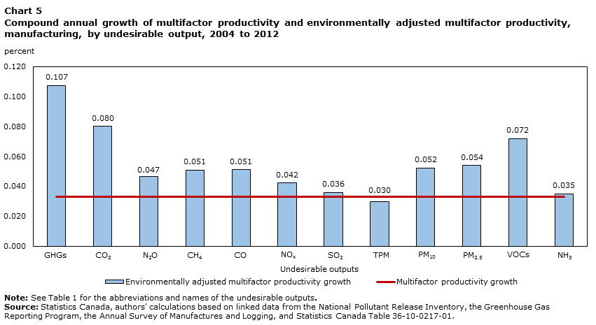
where represents the ratio of gross output of emissions-reporting establishments to the total gross out for all manufacturing establishments. Shares of emissions-reporting establishments in total manufacturing using nominal gross output and GDP averaged over the 2004-to-2012 period are reported in Table A.2 (Appendix A). The results of this adjustment are used to calculate the compound annual growth rates of MFP and EAMFP for each undesirable output, which are shown in Chart 5.
Data table for Chart 5
| Undesirable outputs | Multifactor productivity growth | Environmentally adjusted multifactor productivity growth |
|---|---|---|
| percent | ||
| GHGs | 0.033 | 0.107 |
| CO2 | 0.033 | 0.080 |
| N2O | 0.033 | 0.047 |
| CH4 | 0.033 | 0.051 |
| CO | 0.033 | 0.051 |
| NOX | 0.033 | 0.042 |
| SO2 | 0.033 | 0.036 |
| TPM | 0.033 | 0.030 |
| PM10 | 0.033 | 0.052 |
| PM2.5 | 0.033 | 0.054 |
| VOCs | 0.033 | 0.072 |
| NH3 | 0.033 | 0.035 |
|
Note: See Table 1 for the abbreviations and names of the undesirable outputs. Source: Statistics Canada, authors' calculations based on linked data from the National Pollutant Release Inventory, the Greenhouse Gas Reporting Program, the Annual Survey of Manufactures and Logging, and Statistics Canada Table 36-10-0217-01. |
||
The individual adjustment for each of the undesirable outputs leads to similar or higher estimates of productivity growth for the manufacturing sector, with the exception of TPM, which exhibited slightly lower EAMFP growth (0.030%) than MFP growth (0.033%). The three GHG gases CO2, N2O and CH4 as well as VOCs had the largest differences between MFP and EAMFP growth. It is clear from Equation (14) that the difference between MFP and EAMFP growth is determined by three factors. The first is the relative growth of desirable-to-undesirable output, . If real gross output increases faster than emissions, then EAMFP growth will be higher than MFP growth, which is the case for all emissions except TPM. This is a large part of the reason why EAMFP growth adjusted for total GHGs is much higher than it is for CO2. From 2004 to 2012, emissions of total GHGs fell 11.7% compared to just 4.2% for CO2 while real gross output increased 0.5% for reporting establishments. The second is the undesirable output’s share of total output, , which reflects the relative importance of the emission in total output and is negative in every instance in this analysis. The share of total GHG emissions in total output was relatively stable at 30.4% for the nine-year period. By comparison, the share of N2O in total output was only 0.4%. The last factor is the reporting establishemnt share of gross output in manufactuing, which varies by emission type from 7% to 27% on average over the nine-year period but were nearly identicle for GHGs and N2O. Therefore, even though emissions of N2O declined by 95%, the adjustment to EAMFP growth was less than one fifth as large as that for emissions of total GHGs.
Overall, a decline (increase) in pollution intensity will cause EAMFP growth to be higher (lower) than MFP growth. However, it is both the relative importance of the emissions and the size of the change in emission intensity that determine the magnitude of the difference between EAMFP growth and MFP growth. Strong EAMFP growth, with respect to total GHG emissions, relative to the standard measure of productivity growth reflects its relative importance and its sharp decline relative to a modest increase in real output.
Table 4 shows annual MFP growth rates for the manufacturing sector from 2005 to 2012 in the first row. In the three years around the Great Recession (2007 to 2009), MFP growth was negative, supporting the idea that productivity is procyclical. In the following 12 rows of Table 4, annual percentage-point adjustments to MFP growth attributable to the adjustment to MFP growth for individual undesirable outputs are reported. For example, accounting for CO2 as an undesirable output would increase MFP growth by 0.36 percentage points from 0.559% to 0.919% in 2005. Accounting for N2O, on the other hand, would increase MFP growth by 0.004 percentage points from 0.559% to 0.563%. The bottom row of Table 4 shows the average unweighted contribution to the difference between MFP and EAMFP growth for each year.
| 2005 | 2006 | 2007 | 2008 | 2009 | 2010 | 2011 | 2012 | |
|---|---|---|---|---|---|---|---|---|
| percent | ||||||||
| MFP growth | 0.559 | 0.104 | -0.641 | -0.359 | -1.932 | 1.140 | 0.905 | 0.524 |
| percentage-point adjustment to MFP growth | ||||||||
| Undesirable output | ||||||||
| GHGs | 0.379 | -0.294 | 0.236 | 0.006 | -0.321 | 0.397 | 0.144 | 0.045 |
| CO2 | 0.360 | -0.529 | 0.276 | 0.127 | -0.505 | 0.395 | 0.177 | 0.074 |
| N2O | 0.004 | 0.026 | -0.003 | -0.022 | 0.027 | 0.050 | 0.008 | 0.017 |
| CH4 | 0.033 | 0.070 | 0.043 | -0.003 | -0.081 | 0.020 | 0.004 | 0.056 |
| CO | 0.122 | -0.009 | -0.085 | -0.063 | 0.236 | -0.317 | 0.405 | -0.148 |
| NOX | 0.010 | 0.053 | -0.013 | -0.007 | -0.040 | 0.060 | 0.048 | -0.039 |
| SO2 | 0.002 | 0.008 | 0.014 | -0.007 | 0.007 | -0.008 | -0.001 | 0.005 |
| TPM | -0.010 | 0.035 | -0.026 | 0.005 | -0.017 | 0.049 | -0.032 | -0.031 |
| PM10 | -0.041 | 0.089 | -0.022 | 0.057 | 0.061 | 0.084 | -0.017 | -0.061 |
| PM2.5 | -0.054 | 0.080 | 0.046 | 0.001 | 0.064 | 0.051 | 0.009 | -0.032 |
| VOCs | 0.143 | 0.236 | -0.155 | 0.053 | -0.268 | 0.056 | 0.194 | 0.051 |
| NH3 | 0.003 | -0.011 | -0.016 | 0.003 | -0.005 | 0.038 | -0.003 | 0.006 |
| Unweighted average adjustmentTable 4 Note 1 | 0.062 | 0.021 | -0.002 | 0.005 | -0.031 | 0.046 | 0.083 | -0.023 |
Source: Statistics Canada, authors’ calculations based on linked data from the National Pollutant Release Inventory, the Greenhouse Gas Reporting Program, the Annual Survey of Manufactures and Logging, and Statistics Canada Table 36-10-0217-01. |
||||||||
4.6 Estimates of environmentally adjusted multifactor productivity growth and shadow prices of undesirable outputs for manufacturing subsectors
Estimates of EAMFP growth and shadow prices were produced for eight manufacturing subsectors. The number of undesirable outputs varies from one subsector to the next because of the availability and confidentiality of data for undesirable outputs and economic activity. Some subsectors, such as the two displayed in Table 5, include information for all 12 undesirable output categories. Other subsectors either do not have enough reporting establishments or do not meet the emissions threshold that would require them to report their emissions. Tables similar to Table 5 are shown in Appendix B for most manufacturing subsectors.
| Undesirable output | Paper manufacturingTable 5 Note 1 | Chemical manufacturingTable 5 Note 2 | ||||||
|---|---|---|---|---|---|---|---|---|
| MFP compound annual growth |
EAMFP compound annual growth | Difference | Shadow price |
MFP compound annual growth |
EAMFP compound annual growth | Difference | Shadow price |
|
| percent | $ 2012/tonne | percent | $ 2012/tonne | |||||
| GHGs | 0.42 | 0.38 | -0.04 | -360 | -0.12 | -0.07 | 0.05 | -149 |
| CO2 | 0.42 | 0.41 | -0.01 | -462 | -0.12 | -0.22 | -0.10 | -170 |
| N2O | 0.42 | 0.42 | 0.00 | -87 | -0.12 | -0.10 | 0.02 | -196 |
| CH4 | 0.42 | 0.41 | -0.02 | -413 | -0.12 | -0.11 | 0.01 | -749 |
| CO | 0.42 | 0.51 | 0.08 | -14,083 | -0.12 | -0.14 | -0.03 | -54,533 |
| NOx | 0.42 | 0.43 | 0.01 | -10,786 | -0.12 | -0.11 | 0.00 | -15,922 |
| SO2 | 0.42 | 0.42 | 0.00 | -1,935 | -0.12 | -0.12 | 0.00 | -3,399 |
| TPM | 0.42 | 0.46 | 0.04 | -23,853 | -0.12 | -0.13 | -0.02 | -98,079 |
| PM10 | 0.42 | 0.48 | 0.06 | -48,873 | -0.12 | -0.12 | 0.00 | -296,294 |
| PM2.5 | 0.42 | 0.46 | 0.04 | -49,862 | -0.12 | -0.10 | 0.01 | -388,650 |
| VOCs | 0.42 | 0.43 | 0.00 | -68,620 | -0.12 | -0.13 | -0.01 | -178,707 |
| NH3 | 0.42 | 0.43 | 0.00 | -95,242 | -0.12 | -0.11 | 0.00 | -7,608 |
Source: Statistics Canada, authors' calculations based on linked data from the National Pollutant Release Inventory, the Greenhouse Gas Reporting Program, the Annual Survey of Manufactures and Logging, and Statistics Canada Table 36-10-0217-01. |
||||||||
5 Future research
The growing awareness of the interdependence of economic and environmental performance makes it clear that there is need for further analysis that integrates economic and environmental information at the business establishment level. The results here indicate that accounting for the environmental impact of undesirable outputs sometimes can induce substantial changes in MFP growth. However, expanding the analysis to include industries other than manufacturing and undesirable outputs in addition to GHGs and CACs may reveal more significant implications for EAMFP growth. Moreover, each undesirable output was examined in isolation of the others. Ideally, all outputs, desirable and undesirable, would be assessed together in a single estimation rather than separately, if it were not for econometric limitations. To partly resolve this issue, Cárdenas Rodríguez, Haščič and Souchier (2016) use a random coefficient model to simultaneously estimate the coefficients for multiple undesirable outputs. However, this approach was found to be less practical as the number of undesirable outputs grew to nearly a dozen, mostly because of issues with collinearity and sample size. As found by Cárdenas Rodríguez, Haščič and Souchier (2016), a random coefficient model applied to the data used in this analysis also produced positive shadow prices for some undesirable outputs, in contrast to the intuition that undesirable outputs should have negative prices.
Further work may also focus on how to aggregate undesirable outputs in terms of their costs to producers and society. In addition, it may focus on how undesirable outputs interact with one another as establishments use different abatement strategies. For example, Murty and Russell (2017) argue that multiple undesirable outputs can be jointly produced when there is no trade-off in their production for a given set of inputs, but they rival each other if an increase in emissions of one undesirable output reduces the emissions of another. Consequently, simply adding amounts of undesirable outputs together—even when doing so is relatively straightforward, as in the case of GHGs measured as CO2 equivalents—may produce misleading estimates for shadow prices and EAMFP growth.
In addition, other methodologies for estimating shadow prices need to be tested to further validate the results found here. Those methods may include nonparametric estimates using data envelopment analysis (DEA), as well as parametric estimates using Bayesian estimation and stochastic frontier analysis (SFA). Alternatives to using a Shephard output distance function to characterize production may include directional and hyperbolic distance functions that are often used in DEA and SFA.
An area of examination not covered here might be to look at the role of establishment characteristics and how firm dynamics affect economic and environmental performance. Examining the relative importance of different types of firms (small versus large, foreign-controlled versus domestic-controlled, and entrants and exiters versus incumbents) may provide a rich source of information, particularly for environmental policy development. Moreover, this study focuses on estimating the price of undesirable outputs with respect to production but makes no attempt to estimate their price with respect to society, a far more complex task.
6 Conclusion
Undesirable outputs are an ubiquitous aspect of the environment that in sufficient concentrations can have important social and economic implications. Increasing awareness of how undesirable outputs affect individuals’ longevity and quality of life has motivated significant improvements in data collection and analysis. Growing evidence suggests that the economy and the environment are inextricably linked in such a way that understanding either one of these aspects in isolation is bound to be incomplete and potentially misleading.
This study uses the new NPRI-GHGRP-ASML dataset, which combines information from three sources: the National Pollutant Release Inventory (NPRI), the Greenhouse Gas Reporting Program (GHGRP), and the Annual Survey of Manufacturers and Logging (ASML). This dataset brings together information on environmental and economic activity that enables the interaction of economic activity and the environment to be examined. Specifically, an output distance function was used to derive a shadow price for 12 categories of undesirable outputs individually. The shadow prices of undesirable outputs, in turn, were an essential piece of information for a growth accounting framework to measure how undesirable outputs affect multifactor productivity (MFP) growth, one of the most common measures of the overall performance of an economy. The adjustment provides a measure of environmentally adjusted multifactor productivity growth (EAMFP) for the Canadian manufacturing sector and several manufacturing subsectors.
Some of the key findings are that estimates of shadow prices, and environmental adjustments to MFP growth are broadly consistent with the intuition that prices of undesirable outputs should be negative. More interesting, though, is that the inclusion of undesirable outputs improved productivity growth relative to standard measures, particularly for greenhouse gas (GHG) emissions. In particular, strong EAMFP growth, with respect to total GHG emissions, relative to the standard measure of productivity growth reflects its relative importance and the sharp decline in emissions relative to a modest increase in real output. For almost all of the 12 categories of undesirable outputs, compound annual EAMFP growth was higher than compound annual MFP growth, reflecting improvements in undesirable output intensity.
Appendix A
A.1 A comparison of estimates using gross output and gross domestic product for the manufacturing sector
For comparability purposes, estimates of shadow prices and undesirable output intensities are presented in Table A.1. Estimates of environmentally adjusted multifactor productivity growth and multifactor productivity growth are provided in Table A.2.
| Undesirable outputs | Undesirable output growth coefficient | Shadow price | Undesirable output intensity | |||||
|---|---|---|---|---|---|---|---|---|
| Gross output | GDP | Gross output | GDP | Gross output | GDP | |||
| coefficient | standard deviation | coefficient | standard deviation | $ 2012/tonne | tonnes / $ million 2012 | |||
| GHGs | 0.233 | 0.040 | 0.031 | 0.012 | -390 | -13 | 597.68 | 2,321.36 |
| CO2 | 0.260 | 0.042 | 0.031 | 0.013 | -453 | -14 | 573.56 | 2,227.66 |
| N2O | 0.004 | 0.012 | 0.001 | 0.003 | -1,002 | -92 | 4.06 | 15.93 |
| CH4 | 0.015 | 0.010 | 0.004 | 0.003 | -3,611 | -263 | 4.23 | 33.02 |
| CO | 0.047 | 0.012 | 0.007 | 0.004 | -19,950 | -712 | 2.37 | 9.50 |
| NOx | 0.022 | 0.014 | 0.003 | 0.004 | -34,875 | -1,070 | 0.62 | 2.40 |
| SO2 | 0.005 | 0.008 | 0.002 | 0.003 | -1,489 | -152 | 3.34 | 12.16 |
| TPM | 0.027 | 0.012 | 0.000 | 0.004 | -69,666 | -246 | 0.39 | 1.39 |
| PM10 | 0.036 | 0.009 | 0.003 | 0.003 | -229,573 | -5,146 | 0.16 | 0.55 |
| PM2.5 | 0.025 | 0.008 | 0.002 | 0.003 | -260,042 | -5,230 | 0.10 | 0.34 |
| VOCs | 0.062 | 0.012 | 0.000 | 0.004 | -211,975 | -411 | 0.29 | 1.10 |
| NH3 | 0.017 | 0.012 | 0.002 | 0.003 | -91,780 | -2,411 | 0.18 | 0.70 |
|
Notes: See Table 1 for the abbreviations and names of the undesirable outputs. GDP: gross domestic product. Source: Statistics Canada, authors' calculations based on linked data from the National Pollutant Release Inventory, the Greenhouse Gas Reporting Program, the Annual Survey of Manufactures and Logging, and Statistics Canada Table 36-10-0217-01. |
||||||||
| Undesirable outputs | MFP growth | EAMFP growth | Difference | Shares of emissions-reporting establishments | ||||
|---|---|---|---|---|---|---|---|---|
| Gross output | GDP | Gross output | GDP | Gross output | GDP | Gross output | GDP | |
| percent | ||||||||
| GHGs | 0.033 | 0.102 | 0.107 | 0.108 | 0.074 | 0.006 | 12.7 | 11.5 |
| CO2 | 0.033 | 0.102 | 0.080 | 0.101 | 0.047 | -0.001 | 12.7 | 11.5 |
| N2O | 0.033 | 0.102 | 0.047 | 0.106 | 0.013 | 0.004 | 12.6 | 11.1 |
| CH4 | 0.033 | 0.102 | 0.051 | 0.101 | 0.018 | -0.001 | 12.5 | 11.1 |
| CO | 0.033 | 0.102 | 0.051 | 0.101 | 0.018 | -0.001 | 20.4 | 18.9 |
| NOx | 0.033 | 0.102 | 0.042 | 0.102 | 0.009 | 0.000 | 21.5 | 20.3 |
| SO2 | 0.033 | 0.102 | 0.036 | 0.103 | 0.003 | 0.000 | 13.8 | 13.6 |
| TPM | 0.033 | 0.102 | 0.030 | 0.102 | -0.003 | 0.000 | 17.5 | 16.8 |
| PM10 | 0.033 | 0.102 | 0.052 | 0.103 | 0.019 | 0.001 | 24.0 | 23.8 |
| PM2.5 | 0.033 | 0.102 | 0.054 | 0.103 | 0.021 | 0.001 | 23.9 | 23.9 |
| VOCs | 0.033 | 0.102 | 0.072 | 0.102 | 0.039 | 0.000 | 21.6 | 20.2 |
| NH3 | 0.033 | 0.102 | 0.035 | 0.102 | 0.002 | 0.000 | 7.9 | 7.0 |
|
Notes: See Table 1 for the abbreviations and names of the undesirable outputs. Shares of emissions-reporting establishments in total manufacturing nominal gross output and gross domestic product (GDP) are reported. Growth rates for multifactor productivity (MFP) and environmentally adjusted multifactor productivity (EAMFP) are at compound annual rates calculated as in Chart 5. Source: Statistics Canada, authors' calculations based on linked data from the National Pollutant Release Inventory, the Greenhouse Gas Reporting Program, the Annual Survey of Manufactures and Logging, and Statistics Canada Table 36-10-0217-01. |
||||||||
Appendix B
B.1 Manufacturing subsector estimates
Estimates of multifactor productivity growth from the KLEMS (capital, labour, energy, materials, and services) database for various manufacturing subsectors are included in Table B.1. The estimates of environmentally adjusted multifactor productivity growth reflect how estimates from the KLEMS database would be adjusted if they were to include undesirable outputs with the standard measure of real gross output to form total output. The difference between the two productivity measures is also presented. In the final column, the shadow price for each undesirable output is shown for the year 2012, by subsector.
Most subsectors include information for a limited number of undesirable outputs since not every subsector produces sufficient amounts of each undesirable output to be reported to the National Pollutant Release Inventory and the Greenhouse Gas Reporting Program. In addition, information for some undesirable outputs was suppressed for confidentiality.
| MFP compound annual growth |
EAMFP compound annual growth |
Difference | Shadow price |
|
|---|---|---|---|---|
| percent | $ 2012/tonne | |||
| Food manufacturing (311) | ||||
| CO | 0.12 | 0.11 | -0.01 | -361,445 |
| NOx | 0.12 | 0.12 | 0.00 | -103,893 |
| TPM | 0.12 | 0.11 | 0.00 | -183,037 |
| PM10 | 0.12 | 0.12 | 0.00 | -591,271 |
| PM2.5 | 0.12 | 0.11 | -0.01 | -965,753 |
| VOCs | 0.12 | 0.07 | -0.05 | -135,136 |
| Wood product manufacturing (321) | ||||
| CO | 0.95 | 0.93 | -0.02 | -1,276 |
| TPM | 0.95 | 0.94 | 0.00 | -23,796 |
| PM10 | 0.95 | 0.95 | 0.00 | -65,765 |
| PM2.5 | 0.95 | 0.95 | 0.01 | -79,836 |
| VOCs | 0.95 | 0.93 | -0.02 | -31,421 |
| Paper manufacturing (322) | ||||
| GHGs | 0.42 | 0.38 | -0.04 | -360 |
| CO2 | 0.42 | 0.41 | -0.01 | -462 |
| N2O | 0.42 | 0.42 | 0.00 | -87 |
| CH4 | 0.42 | 0.41 | -0.02 | -413 |
| CO | 0.42 | 0.51 | 0.08 | -14,083 |
| NOx | 0.42 | 0.43 | 0.01 | -10,786 |
| SO2 | 0.42 | 0.42 | 0.00 | -1,935 |
| TPM | 0.42 | 0.46 | 0.04 | -23,853 |
| PM10 | 0.42 | 0.48 | 0.06 | -48,873 |
| PM2.5 | 0.42 | 0.46 | 0.04 | -49,862 |
| VOCs | 0.42 | 0.43 | 0.00 | -68,620 |
| NH3 | 0.42 | 0.43 | 0.00 | -95,242 |
| Petroleum and coal product manufacturing (324) | ||||
| CO | -0.73 | -0.42 | 0.32 | -189,765 |
| NOx | -0.73 | -0.69 | 0.04 | -80,954 |
| PM10 | -0.73 | -0.64 | 0.09 | -1,110,105 |
| PM2.5 | -0.73 | -0.67 | 0.06 | -1,212,031 |
| VOCs | -0.73 | -0.52 | 0.21 | -389,016 |
|
Notes: See Table 1 for the abbreviations and names of the undesirable outputs. EAMFP: environmentally adjusted multifactor productivity. MFP: multifactor productivity. NAICS: North American Industry Classification System. Source: Statistics Canada, authors' calculations based on linked data from the National Pollutant Release Inventory, the Greenhouse Gas Reporting Program, the Annual Survey of Manufactures and Logging, and Statistics Canada Table 36-10-0217-01. |
||||
| MFP compound annual growth |
EAMFP compound annual growth |
Difference | Shadow price | |
|---|---|---|---|---|
| percent | $ 2012/tonne | |||
| Chemical manufacturing (325) | ||||
| GHGs | -0.12 | -0.07 | 0.05 | -149 |
| CO2 | -0.12 | -0.22 | -0.10 | -170 |
| N2O | -0.12 | -0.10 | 0.02 | -196 |
| CH4 | -0.12 | -0.11 | 0.01 | -749 |
| CO | -0.12 | -0.14 | -0.03 | -54,533 |
| NOx | -0.12 | -0.11 | 0.00 | -15,922 |
| SO2 | -0.12 | -0.12 | 0.00 | -3,399 |
| TPM | -0.12 | -0.13 | -0.02 | -98,079 |
| PM10 | -0.12 | -0.12 | 0.00 | -296,294 |
| PM2.5 | -0.12 | -0.10 | 0.01 | -388,650 |
| VOCs | -0.12 | -0.13 | -0.01 | -178,707 |
| NH3 | -0.12 | -0.11 | 0.00 | -7,608 |
| Non-metallic mineral product manufacturing (327) | ||||
| GHGs | -0.53 | -0.45 | 0.08 | -37 |
| CO2 | -0.53 | -0.43 | 0.09 | -42 |
| CO | -0.53 | -0.52 | 0.01 | -7,236 |
| NOx | -0.53 | -0.52 | 0.01 | -1,824 |
| SO2 | -0.53 | -0.53 | 0.00 | -510 |
| TPM | -0.53 | -0.54 | -0.01 | -12,788 |
| PM10 | -0.53 | -0.52 | 0.01 | -33,252 |
| PM2.5 | -0.53 | -0.50 | 0.03 | -48,727 |
| VOCs | -0.53 | -0.53 | 0.00 | -209,124 |
| Primary metal manufacturing (331) | ||||
| GHGs | -0.04 | -0.02 | 0.02 | -197 |
| CO2 | -0.04 | -0.09 | -0.05 | -240 |
| N2O | -0.04 | -0.03 | 0.02 | -2,171 |
| CH4 | -0.04 | -0.05 | -0.01 | -3,584 |
| CO | -0.04 | -0.14 | -0.10 | -3,736 |
| NOx | -0.04 | -0.05 | 0.00 | -32,190 |
| SO2 | -0.04 | -0.04 | 0.00 | -359 |
| TPM | -0.04 | -0.07 | -0.02 | -25,129 |
| PM10 | -0.04 | -0.08 | -0.04 | -72,248 |
| PM2.5 | -0.04 | -0.06 | -0.02 | -76,973 |
| VOCs | -0.04 | -0.01 | 0.03 | -458,398 |
| Transportation equipment manufacturing (336) | ||||
| PM10 | -0.57 | 2.33 | 2.90 | -14,019,487 |
| PM2.5 | -0.57 | 1.35 | 1.92 | -16,435,588 |
| VOCs | -0.57 | 1.69 | 2.26 | -699,141 |
|
Notes: See Table 1 for the abbreviations and names of the undesirable outputs. EAMFP: environmentally adjusted multifactor productivity. MFP: multifactor productivity. NAICS: North American Industry Classification System. Source: Statistics Canada, authors' calculations based on linked data from the National Pollutant Release Inventory, the Greenhouse Gas Reporting Program, the Annual Survey of Manufactures and Logging, and Statistics Canada Table 36-10-0217-01. |
||||
References
Aiken, D.V. and C.A. Pasurka Jr. 2003. “Adjusting the Measurement of US Manufacturing Productivity for Air Pollution Emissions Control.” Resource and Energy Economics 25: 329–351.
Baldwin, J.R., W. Gu, R. Macdonald, and B. Yan. 2014. What is Productivity? How is it Measured? What has Canada’s Performance Been over the Period 1961 to 2012? The Canadian Productivity Review, no. 38. Statistics Canada Catalogue No. 15-206-X. Ottawa: Statistics Canada.
Brandt, N., P. Schreyer, and V. Zipperer. 2014. Productivity Measurement with Natural Capital and Bad Outputs. OECD Economics Department Working Papers, no. 1154. Paris: OECD Publishing.
Cárdenas Rodríguez, M., I. Haščič, and M. Souchier. 2016. Environmentally Adjusted Multifactor Productivity: Methodology and Empirical Results for OECD and G20 Countries. OECD Green Growth Papers, no. 2016-04. Paris: OECD Publishing.
Coelli, T.J., and S. Perelman. 1996. Efficiency Measurement, Multiple-output Technologies and Distance Functions: With Application to European Railways. CREPP Discussion Paper no. 96/05. Liège, Belgium: University of Liège.
Coelli, T.J., and S. Perelman. 1999. “A comparison of parametric and non-parametric distance functions: With application to European railways.” European Journal of Operational Research 117 (2): 326–339.
Coelli, T.J., D.S.P. Rao, C.J. O’Donnell, and G.E. Battese. 2005. An Introduction to Efficiency and Productivity Analysis. 2nd edition. New York: Springer.
Dang, T., and A. Mourougane. 2014. Estimating Shadow Prices of Pollution in OECD Economies. OECD Green Growth Papers, no. 2014-02. Paris: OECD Publishing.
ECCC (Environment and Climate Change Canada). National Pollutant Release Inventory. 2015. 2015 Summary Report: Reviewed Facility-reported Data. Gatineau, Quebec: ECCC.
Färe, R., and S. Grosskopf. 1990. “A distance function approach to measuring price efficiency.” Journal of Public Economics 43: 123–126.
Färe, R., S. Grosskopf, C.A.K. Lovell, and S. Yaisawarng. 1993. “Derivation of shadow prices for undesirable outputs: A distance function approach.” The Review of Economics and Statistics 75 (2): 374–380.
Färe, R., and D. Primont. 1995. Multi-output Production and Duality: Theory and Applications. Boston: Kluwer Academic Publishers.
Murty, S., and R. Russell. 2017. Bad Outputs.
Working paper. Available at:
http://economics.ucr.edu/people/profemer/russell/bad_outputs_june26.pdf (accessed March 9, 2018).
Shephard, R.W. 1970. Theory of Cost and Production. Princeton: Princeton University Press.
Statistics Canada. n.d. Table 36-10-0217-01 Multifactor productivity, gross output, value-added, capital, labour and intermediate inputs at a detailed industry level. Available at: https://www150.statcan.gc.ca/t1/tbl1/en/tv.action?pid=3610021701 (accessed December 12, 2018).
Stern, N. 2008. “The economics of climate change.” American Economic Review 98 (2): 1–37.
Stiglitz, J., A. Sen, and J.-P. Fitoussi. 2009. Report by the Commission on the Measurement of Economic Performance and Social Progress. Paris. Available at: http://ec.europa.eu/eurostat/documents/118025/118123/Fitoussi+Commission+report (accessed December 12, 2018).
Syverson, C. 2011. “What determines productivity?” Journal of Economic Literature 49 (2): 326–365.
WCED (World Commission on Environment and Development). 1987. Our Common Future. Oxford: Oxford University Press.
- Date modified: