
Analytical Studies: Methods and References
Mapping Production Activity in Yukon: Experimental Indexes of Grid Square-based Gross Domestic Product
Skip to text
Text begins
Acknowledgements
The authors would like to thank Karen Wilson, Danny Leung, Bishnu Saha, Peter Murphy and participants at the 69th North American Meetings of the Regional Science Association International, held in Montréal in November 2022, for their helpful comments.
Abstract
In recognition that more geographically granular economic data improves our ability to understand the nature of production, support regional economies, and address emerging socio-economic and environmental problems, statistical agencies are increasingly asked to produce gross domestic product (GDP) estimates at finer levels of geography. This demand is being met in different ways around the world, with, for instance, the European Union producing GDP estimates at the Nomenclature of Territorial Units for Statistics level and the United States producing GDP estimates at the county level. While Canada produces GDP estimates for census metropolitan areas, it does not currently produce the same level of coverage for smaller geographies as does the European Union or the United States. This paper addresses this gap by developing subprovincial and subterritorial grid square-based GDP using Yukon as a test case. Yukon was chosen because its small resource- and government-based economy provides a challenging but comprehendible test of these fine-grained measures. This choice will also support ongoing work measuring the economies of circumpolar regions. With this in mind, the paper has three objectives. First, it introduces and discusses the benefits a fixed grid for measurement. Second, it discusses how the measurement of fine-level aggregates relates to concepts within the System of National Accounts. Third, it identifies the types of data necessary to estimate GDP across a 1 km2 grid and produces a set of grid-based GDP estimates that serve to describe the geography of economic output in Yukon.
1 Introduction
Greater geographic granularity improves analysts’ and policy makers’ ability to recognize issues, understand the nature of production and support regional economies. For over two decades, researchers have explored innovative methods for estimating gross domestic product (GDP) at fine geographies. These studies can broadly be divided into studies using sensor-based data (Ru et al. 2023, Ghosh et al. 2010, Yue et al. 2014, Doll et al. 2006, Chen et al. 2002) and studies based on population data (Murakami and Yamagata 2019, Kummu et al. 2018, Nordhaus 2008, 2006). The goal has often been to produce a global map of how economic activity is distributed across regions to illustrate the utility of presenting GDP for small areal units.
The use of readily available sensor-based and population data is advantageous, because the geolocation of GDP can occur across the entire surface of the earth. The drawbacks are that the allocation models do not exactly align with the notion of GDP, and industrial information is missing. Studies using night-based luminosity (Ghosh et al. 2010, Doll et al. 2006, Chen et al. 2002) must assume that GDP occurs where lights are present. This method focuses attention on cities while limiting or omitting the production that occurs in rural areas (on farms, at hydro plants, at mines and in forests). Moreover, since these studies assume that GDP is dispersed per lumen, a downtown core or entertainment area with many lights will be accorded more GDP than an airport or manufacturing district that is more dimly lit. Similarly, studies based on population (Murakami and Yamagata 2019, Nordhaus 2008, 2006) assume that GDP and population are synonymous. Therefore, they will also overestimate GDP of populated grid squares and underestimate GDP of unpopulated areas such as rural locations, industrial parks or ports. These concerns can be partially addressed by adding additional sensor data (on agriculture, airports and roads) (Ru et al. 2023, Murakami and Yamagata 2019, Yue et al. 2014), but this is only a partial adjustment because only specific industries and assets will be accounted for.
Statistical agencies are also producing GDP estimates at finer and finer levels of geography. These estimates are made from the internal datasets of national statistics offices (NSOs) in different ways around the world and are based on political areas rather than fixed areal units. The European Union now produces GDP estimates based on the Nomenclature of Territorial Units for Statistics (Eurostat 2022 a, b, c), while the United States produces county-level GDP estimates (Bureau of Economic Analysis, 2022). Statistics Canada produces GDP estimates for census metropolitan areas (CMAs) (Statistics Canada, 2022a) but does not currently produce the same type of consistency for smaller geographies as does the European Union or the United States. These estimates geospatially locate GDP in a more production-consistent manner than sensor- or population-based allocation models and can potentially be used to produce industry estimates. But they lack the specificity of the small area fixed grids.
This paper spans the academic work and estimation strategies used in NSOs. It addresses the issue of producing fine, grid-level geography estimates for Canada by exploring the measurement of subprovincial and subterritorial GDP using Yukon as a test case. The goals of the paper are threefold. First, it introduces a fixed grid for measuring Canadian GDP. This grid is measured at a 1 km2 resolution to improve granularity of subterritorial estimates. Second, the paper discusses how the measurement of fine-level aggregates relates to concepts within the System of National Accounts 2008 (SNA 2008) (United Nations et al., 2008). It illustrates how internal NSO datasets can be combined with allocation models to produce geospatially disaggregated values by industry. Third, the paper identifies the types of data necessary to estimate GDP at such a fine resolution and produces a set of estimates based on a 1 km2 grid. These estimates are then shown on maps and used to produce urban–rural GDP estimates for Yukon.
Covering 472,345 km2(Statistics Canada, n.d.), Yukon is larger than California (423,967 km2) (Census Bureau, n.d.) and only marginally smaller than France (547,557 km2) (World Bank, n.d.). Despite its size, in 2021, it had a population of just over 40,000 people (Statistics Canada, 2022b) who produced $2.9 billion in GDP (in 2012 dollars) (Statistics Canada(n.d.). In many parts of the world, this population would be comparable to that of a moderately sized town. Despite its small population, Yukon was chosen as a test case for several reasons. First, its small but broad-ranging resource- and government-based economy provides a challenging test requiring multiple sources and methods to allocate GDP to grid squares. Second, it is possible, given the small size of its economy, to use ground truth to assess whether the estimates make sense, and there are numerous secondary sources to do this. Lastly, Yukon was chosen to support ongoing work measuring the economies of circumpolar regions.
Each of the paper’s three goals is discussed within a separate section of the paper. The use of a fixed grid is discussed in Section 2, while the relationship between fine geographies and the notions of GDP in the SNA 2008 is explored in Section 3. Section 4 discusses how measurement is undertaken. Section 5 illustrates several sample outputs and examines issues for publishing fine-level data. Section 6 concludes.
2 Census geographies versus fixed grids for measuring gross domestic product
GDP is used to measure economic growth over time and compare the size of economies across space. Internationally, NSOs accomplish this by measuring GDP within national borders, while domestically this is done by using subnational administrative units like provinces, states or counties. Once the decision is made to measure GDP for finer-grained geographic areas, such as employment zones within a city or areas susceptible to flooding, administrative boundaries begin to make less sense. An ideal system of measurement would facilitate placing GDP where production occurs and use geometries that are sufficiently detailed so that economic relationships, such as the relationship between infrastructure investment and economic growth, can be more effectively measured and tested.Note
Within Canada, the traditional starting point for small area geographic information is the dissemination area (DA). A DA is defined as
… a small, relatively stable geographic unit composed of one or more adjacent dissemination blocks with an average population of 400 to 700 persons based on data from the previous Census of Population Program. It is the smallest standard geographic area for which all census data are disseminated. DAs cover all the territory of Canada (Statistics Canada 2021).
While typically populated, DAs can have no population. Importantly, because they must cover the land mass of Canada and the population of Canada is not equally distributed, some units cover very large areas but have few (if any) people, while others may have a large number of individuals but a small area. As a general rule, urban geographies are fine grained. This can be seen in Figure 1 for Yukon, where very large areas are covered by one DA, with much smaller DAs encompassing or dividing up more populated areas like Whitehorse. In addition to varying in size, DAs also have irregular shapes. As Statistics Canada (2021) explains, “DA boundaries usually follow permanent and visible features on the ground, such as roads, railways, water features and power transmission lines. A small number of DA boundaries also follow imaginary lines, such as street extensions, utility or transportation easements, and property lines.”
The highly varying sizes and shapes of DAs limit their capacity for analysis. First, the units have greatly differing shapes and areas that, while having a utility for population studies, are of limited use for integration with other data sources that are often finer grained (e.g., climate or land use data). Perhaps more important, geographically large DAs are of more limited analytical use beyond the Census of Population. This limitation occurs because the census geographic boundaries are conditional on the needs of the census rather than the information being analyzed. As Figure 1 illustrates, there are four DAs that cover most of Yukon’s land mass, with many population centres stamped out of them. For economic activities that do not follow populations closely (e.g., resource extraction and infrastructure-driven GDP such as utilities), the geographic resolution of DAs is insufficient to meaningfully represent where economic activity is taking place. Consequently, it is not possible to consistently relate with geospatial precision events that may affect an economic activity (e.g., flooding or forest fires) with production locations (e.g., road networks, industrial parks and logging sites) and the effect of the events (e.g., production disruptions or pollution of adjacent rivers).
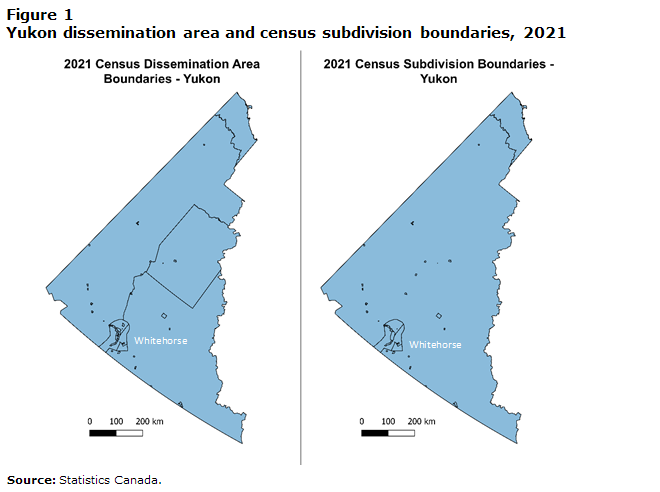
Description for Figure 1
Figure 1 shows two maps side by side. The left-hand map shows the census dissemination areas for Yukon from the 2021 Census of Population. The right-hand map shows the census subdivisions for Yukon from the 2021 Census of Population. Whitehorse is labelled on both maps. Below each map is a scale showing the distance from 0 km to 200 km. The census subdivisions and census dissemination areas are shown to cover the complete landmass of Yukon with irregular shapes. Areas with larger populations resemble small, often irregular shapes that are stamped out of larger irregular shapes. The same effect is seen in both maps.
Current census geography aggregation structures use DA boundaries to build up to census subdivisions (CSDs) (see Figure 1), CMAs or economic regions (ERs) (Statistics Canada 2021). The higher-level aggregations have irregular boundaries that are subject to change across census cycles and can overlap (e.g., CMA and ER boundaries). The result is an analysis that must be conditioned on a census cycle; this can present considerable issues for residual disclosure when used with the business data that underlie GDP estimation.
The use of a fixed grid alleviates a majority of these problems and brings additional benefits. A fixed grid:
- allows for standardized and simplified analysis
- helps to mitigate (Arbia 1989) and test for sensitivity of results to the modifiable areal unit problem (see Bemrose et al. 2017)
- smooths out irregularities arising from population densities
- presents values that are truer to a real-world representation
- does not condition on the population when linking with other spatial data
- does not require conditioning on a census period (Lloyd et al. 2017).
The use of a fixed grid also supports the release of information that respects the confidentiality provisions of the Statistics Act while presenting consistent intertemporal and spatial information. The use of small areas presents challenges for preserving confidentiality, in particular for business data, where 1 km2 grid squares often contain just a few businesses, especially in rural, sparsely populated areas. However, methods like random tabular adjustment and the use of open-source data can help to overcome these issues. Moreover, once in a publishable state, the grid values can be aggregated into any other geography or geometry that is desired. And, since the grids provide a standardized unit of measure that can be used to link data from multiple domains (e.g., weather or environment, topographical features, human activity, business activity, or health), the releasable estimates support the integration of GDP into the multidisciplinary examinations of phenomena that are increasingly required.
3 Gross domestic product for fine geographies
To measure GDP based on a fixed grid, it is assumed that each grid square constitutes a separate economy and that the productive activity of institutional units (e.g., firms and governments) can be measured or allocated by grid square. This creates a predominantly bottom-up approach based on firm-level data for most industries that differs from the existing literature, which uses a top-down approach to allocate industry or regional GDP estimates to a grid square (Ru et al. 2023, Ghosh et al. 2010, Murakami and Yamagata 2019, Yue et al. 2014, Doll et al. 2006, Nordhaus 2008, 2006, Chen et al. 2002). In deciding to begin with institutional units, the approach used here builds on the datasets for estimating GDP housed within NSOs. These baseline concepts then align with the recommendations of the SNA 2008 and the sixth edition of the Balance of Payments and International Investment Position Manual (BPM6). These manuals, especially the latter, have recommendations that focus on methods for measuring institutional units that cross geographical boundaries and others for dealing with multiterritory units.
This alignment is important, because the credibility of the grid square GDP estimates presented in this paper rests on their consistency with national accounting concepts, without which they would not be accepted by the agency or the analysts and policy makers who use agency data. Therefore, some time is spent in this paper drawing out these connections. Readers more interested in the concrete steps taken to develop grid-based GDP and what these estimates look like can skip to the next section without any loss of continuity.
The SNA 2008 and BPM6 have largely been created with the goal of developing statistics based on resident institutional units that are active within nation-states or governed areas. For example, SNA 2008 section 4.12 states:
Economic territory has the dimensions of physical location as well as legal jurisdiction. The concepts of economic territory and residence are designed to ensure that each institutional unit is a resident of a single economic territory. The use of an economic territory as the scope of economic statistics means that each member of a group of affiliated enterprises is resident in the economy in which it is located, rather than being attributed to the economy of location of the head office.
This creates dual criteria for an economy that includes legal and geographic considerations. In discussing which institutional units to identify with an economy, the SNA 2008 (4.10) also notes:
The residence of each institutional unit is the economic territory with which it has the strongest connection, in other words, its centre of predominant economic interest. The concept of economic territory in the SNA coincides with that of the BPM6. Some key features are as follows. In its broadest sense, an economic territory can be any geographic area or jurisdiction for which statistics are required. The connection of entities to a particular economic territory is determined from aspects such as physical presence and being subject to the jurisdiction of the government of the territory. The most commonly used concept of economic territory is the area under the effective economic control of a single government. However economic territory may be larger or smaller than this, as in a currency or economic union or a part of a country or the world.
While geared towards larger areas with a notion of political control, the SNA and BPM6 do note that statistics can be generated for any area of interest. The small, fixed grid squares discussed here therefore fall within their definition of economic territory, albeit towards its logical extreme. Nevertheless, the recommendations from the manuals still apply and the grid based economic area / economic territory can be used to determine which institutional units are active within it. The measurement is most clearcut for small businesses that are the institutional units in question and which have a single location that can be located within a grid square. However, it poses some challenges for the use of grids in cases where the production by an institutional unit occurs over a large area.
There are four cases where this occurs. The first is natural resource use and extraction, where production activity takes place over large and often remote areas. The second is production that occurs over networks (e.g., communications, railways, trucking or airlines). The third is production that occurs within large, complex firms. The fourth is public sector production, in particular public administration.
To implement measurement of production within the grid for these cases, the notion of a multiterritory institutional unit is adopted. The multiterritory unit is discussed in BPM6, which states:
In the case of a multiterritory enterprise, it is preferable that separate institutional units be identified for each economy, as discussed in paragraphs 4.26–4.33. If that is not feasible because the operation is so seamless that separate accounts cannot be developed, it is necessary to prorate the total operations of the enterprise into the individual economic territories. The factor used for prorating should be based on available information that reflects the contributions to actual operations. For example, equity shares, equal splits, or splits based on operational factors such as tonnages or wages could be considered. Where taxation authorities have accepted the multiterritory arrangements, a prorating formula may have been determined, which should be the starting point for statistical purposes. Although the situation is somewhat different from the case of joint administration or sovereignty zones, discussed under economic territory in paragraph 4.10, the solution of prorating may be the same.
The proration of the enterprise means that all transactions need to be split into each component economic territory. The treatment is quite complex to implement. This treatment has implications for other statistics and its implementation should always be coordinated for consistency. Compilers in each of the territories involved are encouraged to cooperate to develop consistent data, avoid gaps, and minimize respondent and compilation burden, as well as assist counterparties to report bilateral data on a consistent basis.
In the four cases, different methods of prorating (imputing or allocating) are employed depending on the type of production present. This allows each grid to be treated as a separate economy for which a GDP value can be computed.
4 Measuring spatial gross domestic product
This section discusses the methods used to determine GDP of a particular grid square at a 1 km2 resolution for Yukon. The discussion blends methods and data sources because, depending on the type of production activity, a different form of measurement is used. The form of measurement is based on the way production occurs, and this dictates the type of data that is required. Because there are different approaches, the terms “prorate,” “impute” and “allocate” are used synonymously depending on the source or how they are commonly used for the models employed.
There are four forms of measurement for determining GDP by grid square:
- direct measurement of business activity
- imputations for remote workplaces and natural resources activity
- imputations for production on networks
- imputations for public sector activity.
The starting point for measurement is the supply and use tables produced by the Industry Accounts Division at Statistics Canada and the firm-level microdata compiled by the Economic Analysis Division. In all cases, GDP measurement is benchmarked to GDP at basic prices estimated by industry. For firm-level data, income-based GDP estimates formed by summing compensation of employees, gross operating surplus, taxes less subsidies on production and mixed income are compiled from administrative files and benchmarked to supply and use tables. They form the basis for the first approach. When this method is used, activity is geolocated to grid squares based on latitude and longitude from Statistics Canada’s Business Register (BR). For the second, third and fourth methods, different forms of spatial information (e.g., road networks, power grids, building footprints and school enrolments) are used to spread industry-level GDP estimates from the supply and use tables to the appropriate grid squares based on spatially appropriate allocation models determined by available data on that industry.
The subsequent subsections discuss the four different forms of measurement in greater detail. They explain why certain types of measurement are appropriate and why certain data sources are needed to facilitate this measurement. Table 1 reports the type of measurement used and the relevant data sources for a selected set of industries to illustrate the five forms of measurement. A full listing of industries is found in the appendix (see Appendix Table A.1).
| NAICS code | Label | Measurement type | Source | Description | Vector | Approach |
|---|---|---|---|---|---|---|
| 111 | Crop production | Natural resources imputation | GeoYukon | Agricultural areas | Polygons | Allocate based on weight = area per grid cell/total area |
| 21222 | Gold and silver ore mining | Natural resources imputation | GeoYukon mining and exploration activities per |
Hardrock mining locations Personal communication: Sydney.VanLoon@yukon.ca, Yukon Geological Survey | Points | Use points per grid cell/total points |
| 2211 | Electric power generation, transmission and distribution | Network imputation | Atlas of Canada Remote Communities Energy Database | Natural Resources Canada's Remote Communities Energy Database | Points | Use 0.75 × energy (kw) per grid cell/total kw |
| GeoYukon Yukon Energy Corporation Power Lines | GeoYukon | Lines | Use 0.25 × length per grid cell/total length | |||
| GeoYukon Yukon Energy Corporation Distribution Lines | GeoYukon | Lines | Use 0.25 × length per grid cell/total length | |||
| 31 | Manufacturing | Direct measurement/ firm allocation | GDP by firm size file | Small firms: Unit locations Complex firms: Allocation model | Points | Allocate based on unit values in grid |
| 481 | Air transportation | Network imputation | Our Airports | List of Yukon airports with their size and coordinates | Points | Use size of airport |
| 484 | Truck transportation | Network imputation | Census of Population | Road Network File | Lines | Use rank × length per grid cell/total length |
| 6111 | Elementary and secondary schools | Public sector imputation | Open government enrolment data | Enrolment by school and grade for all Yukon schools Combination of different Internet searches to find the school locations | Points Coordinates for schools | Use enrolment/total enrolment |
| 622 | Hospitals | Public sector imputation | Combination of different Internet searches to find the hospital locations | Coordinates for hospitals | Points | Use number of beds |
| 911 | Federal government public administration | Public sector imputation | Directory of Federal Real Property | Directory of Federal Real Property | Points or polygons | Use buildings per grid cell/total buildings |
| 914 | Aboriginal public administration | Public sector imputation | Open Data Canada First Nations Locations | Points | First Nations geographic locations | Use points per grid cell/total points |
|
Notes: NAICS = North American Industry Classification System; GDP = gross domestic product. Source: Statistics Canada. |
||||||
4.1 Direct measurement
Direct measurement is the most common type of measurement and is typically applied to industries where business activity is attributable to specific locations (e.g., manufacturing [North American Industry Classification System (NAICS) 31 to 33], wholesale trade [NAICS 41] and retail trade [NAICS 44 to 45]). It relates business activity to a business location based on information from the BR, a comprehensive statistical frame that provides information on the size (e.g., employment) and structure of businesses, from the full enterprise down to individual statistical (operating) locations that are geocoded. In urban areas, geolocation data are accurate at the block-face level. However, for rural locations and many small towns, the postal code information employed to geolocate firms is less precise leading to less accuracy.
Based on these structures, two types of direct measurement are employed, both of which come from files designed to measure GDP by firm size that link to the BR. The first type is for small businesses. They are single-location firms that can be geolocated using latitude and longitude coordinates from the BR. In these cases, GDP of the firm is located in the grid square where it falls.
The second type is for complex businesses. They can be multilocation businesses in the BR that correspond with the notion of a multiterritory enterprise from the BPM6. The value added for these businesses is calculated at the ultimate parent level (highest level possible) and then allocated through the different levels recorded in the BR to reach the location level based on employment values or the number of business locations.
Allocation is performed for incorporated firms based on employment and the structure of the firm. Large firms have a structure on the BR that resembles an organization chart. Employment values can be recorded at any node but are typically recorded above production or service locations. In some cases, the BR provides estimates for employment by location. This information is used to help split values when it is present. When it is missing, an assumption that value added is equally split between locations is imposed. Non-employment variables such as profits are typically reported by a node that is high in the firm organization, such as a head office. These values are spread to locations based on employment and payroll values. In some cases, there may be missing values, and they are imputed at the location level using Markov chain imputation (Yuan, 2010). GDP values are then calculated and benchmarked to the industry-level values from the supply and use tables. Finally, the value of GDP for the location is located in the grid where it falls.
4.2 Remote workplace and natural resource imputations
GDP for remote workplaces and natural resources is predominantly reported where tax reporting locations are listed in Statistics Canada’s data collection system. For major mining companies, reporting is likely to occur from their head office located in a major urban centre outside Yukon. For forestry companies, reporting does not occur in the timber harvest area. For agricultural activities, reporting occurs from farm or corporate head offices and not necessarily where agricultural production takes place.
To produce grid-based GDP estimates, it is therefore necessary to choose a method for allocating GDP to grid squares based on where an activity occurs.Note Current data collection systems do not collect sufficiently detailed data to allow for this to be done at a firm level for all industries. Rather, allocations are made based on spatial data that coincide with the primary activity by NAICS code. In cases where point information can be obtained, it is used as a starting point. Points are production locations in remote areas, such as mine sites, where the latitude and longitude of the location can be determined. Points are typically used when dealing with resource industries found in NAICS 21 (mining, quarrying, and oil and gas extraction). However, in some cases it is more appropriate to allocate GDP along lengths (lines) or within areas (polygons). Lengths are used, for example, when gold mining occurs along waterways, where the value is spread along the length of the rivers where the placer mining takes place. Finally, for some activities, polygons are used. Polygons represent enclosed areas such as farm fields (crop production [NAICS 111]) or pastures (animal production and aquaculture [NAICS 112]), as well as areas where there are forestry cuts (forestry and logging [NAICS 113]). For support activities, there is no indication for where the activities occur. These values are spread across the grid squares under the assumption that support activities for these industries occur where production of their associated industry takes place.
4.3 Network imputations
In several industries, production occurs on networks. This includes transportation networks, power generation and transmission networks, communication networks, and water and sewer networks. In these cases, spatial information related to network capital is used to allocate GDP values to grid squares. These allocation models use network-size, node and edge information to enrich the models. For example, the allocation model for truck transportation (NAICS 484) uses information on the road network in conjunction with information on road quality. In this way, paved highways are given a higher weighting than unpaved roads or lower-order surface streets. Similarly, airport capacity is used to spread air transportation (NAICS 481) GDP among Yukon airports and aerodromes.
4.4 Public sector imputations
Public sector GDP is composed of public administration (NAICS 91) and the public portions of educational services (NAICS 61) and health care and social assistance (NAICS 62). The latter two are predominantly composed of the public school system and hospitals.
Public sector activity in the BR is recorded at higher levels within organizations. For example, educational services activities are recorded by the school board or ministry of education, depending on the jurisdiction. As a result, using data based on tax filing locations will not cover public sector locations properly. To address this issue, public sector GDP is imputed to the locations where production occurs using geospatial information on building sizes (NAICS 91), data on enrolment in schools from open datasets published by the Government of Yukon (NAICS 61), and information on the number and location of hospital beds published by the Government of Yukon (NAICS 62).
Based on these four imputation methods, industry-level GDP from the provincial and territorial accounts is allocated to individual grid squares. This ensures that the grid-square estimates add up to published territorial GDP estimates. Across the four methods, 58.4% of GDP is allocated based on direct measurement, while imputations based on spatial allocation models are employed for the remaining share. Of these, the imputation for the public sector (35.1%) is the largest (see Table 2).
| Remote workplaces | Networks | Direct observation | Public sector | |
|---|---|---|---|---|
| Percent of GDP | 3.6 | 2.9 | 58.4 | 35.1 |
|
Note: GDP = gross domestic product. Source: Statistics Canada. |
||||
5 Results
Presented below is a set of figures aimed at illustrating the geography of Yukon’s GDP distributed by grid square. Presenting grid square estimates raises the problem of meeting confidentiality guidelines, as many will have only a few businesses. To address this problem, the levels of grid square GDP are not reported—instead, grid squares are shaded to indicate relative intensity of production or simply coloured black to indicate the presence of activity. While this approach is unsatisfactory if the estimates are to be compared with grid square GDP estimates elsewhere or over time, it does provide the reader with a clear sense of where production is occurring and where it is most intense.
To provide an overview, Figure 2 presents the geographic distribution of Yukon’s GDP aggregated to a 10 km2 grid square resolution. These larger grid squares are used because the sheer size of Yukon makes presenting the data with smaller grid squares difficult, in particular when using colour to indicate intensity of economic output. Unlike sensor-based or population-based estimates for the spatial distribution of economic activity, Yukon’s spatial GDP pattern closely follows the road network and production in mining areas around Dawson City, which are coloured darker blue to indicate lower GDP levels. Similar to sensor- or population-based estimates, populated areas, such as Whitehorse and Dawson City, are orange to indicate higher GDP levels. These patterns come from the imputation methods used for network values that place GDP to the locations where the productive activity is occurring. They reflect the way in which economic dispersion is closely tied to society’s ability to move goods around and highlight the importance that infrastructure networks have for supporting the economy. These patterns also reflect the stylized fact that density of population and density of networks are associated with higher GDP (the road, water, sewer, electrical and telecommunications grids are all densest in more heavily populated areas).
The highest GDP values occur in and around Whitehorse and Dawson City. They are two of the most populated centres in the territory and contain the largest number of businesses and important public sector entities. Much of the placer gold mining in Yukon occurs in the rivers around Dawson City. Public sector entities in the territory, including the territorial government, the hospital and Yukon University are all located in Whitehorse. Smaller communities have fewer businesses, often in the service sector (e.g., hotels, service stations and retail stores) and also include public sector activity, such as police detachments, schools and health centres, which generate GDP.
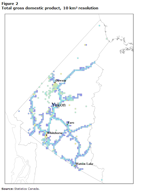
Description for Figure 2
Figure 2 shows a map of Yukon with parts of Alaska, the Northwest Territories and British Columbia included to help show the shape of Yukon. The map has a white background that is overlaid with coloured squares that represent 10 km2. Only squares with a non-zero value are shown. Whitehorse, Dawson, Faro and Watson Lake are labelled on the map.
The grid squares follow map colouring from dark blue (low) to red (high) to show the relative value of gross domestic product across Yukon. The largest values (the red values) are shown in the cities and towns, with the brightest red value being in Whitehorse. Lower-value, blue grid squares are found in and around smaller communities and along the road and electrical transmission grids. The area around Dawson where placer mining occurs on rivers and streams is also illustrated in this way. Overall, the grid squares illustrate geospatial usage of infrastructure, mining in remote locations and denser economic activity in populated areas.
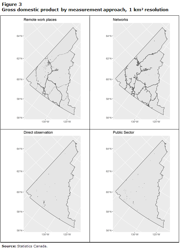
Description for Figure 3
Figure 3 is a panel that shows four maps. The panel is two maps wide and two maps high. All maps show the outline of Yukon and grid squares that have a non-zero value. The maps include latitude lines in the background from 56 degrees north to 64 degrees north and longitude lines of 130 degrees west and 125 degrees west.
The top-left map is labelled “Remote workplaces.” It shows the grid squares associated with forestry, agriculture and mining. Many of these squares follow the road networks or the rivers and creeks where placer mining occurs.
The top-right map is labelled “Networks.” It shows the grid squares associated with transportation, electricity production and distribution, water and sewer, and other network-based industries. For this map, the grid squares follow the physical infrastructure associated with the production activity, and the road network can be understood from the values.
The bottom-left map is labelled “Direct observation.” It shows grid squares associated with gross domestic product that is generated at a business location. These grid squares are predominantly associated with population centres, with the largest concentration of grid squares being shown around Whitehorse.
The bottom-right map is labelled “Public sector.” It shows grid squares associated with public sector activity: health, education and public administration. The majority of these grid squares are associated with population centres.
Comparing across the four maps, the geospatial patterns indicate that grid squares associated with networks and remote workplaces are widely distributed, while grid squares associated with direct observation or the public sector are concentrated around population centres.
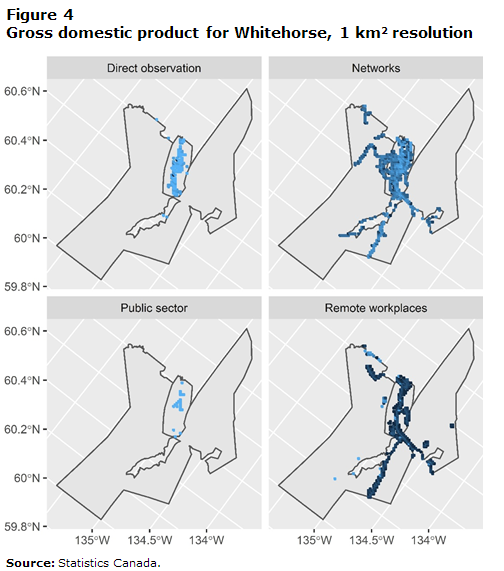
Description for Figure 4
Figure 4 is a panel that shows four maps. The panel is two maps wide and two maps high. All maps show the outline of the Whitehorse census subdivision and the Whitehorse, unorganized census subdivision. The non-zero value grid squares are shown along a light-blue (high) to dark-blue (low) colour gradient. The maps include latitude lines in the background from 59.8 degrees north to 60.6 degrees north and longitude lines of 135 degrees west, 134.5 degrees west and 134 degrees west.
The top-left map is labelled “Direct observation.” It shows grid squares associated with gross domestic product (GDP) generated at a business location. These grid squares are predominantly associated with the central areas of Whitehorse; they are the lightest blue tones across the four maps and indicate the highest GDP values.
The top-right map is labelled “Networks.” It shows the grid squares associated with transportation, electricity production and distribution, water and sewer, and other network-based industries. These squares are medium blue tones, indicating mid-level GDP values. They are spread across the space more broadly than grid squares based on other types of measurement, reflecting the use of infrastructure capital as an allocation method.
The bottom-left map is labelled “Public sector.” It shows grid squares associated with public sector activity: health, education and public administration. These grid squares are associated with the populated areas of Whitehorse and are consistently light blue, indicating higher values of GDP.
The bottom-right map is labelled “Remote workplaces.” It shows grid squares associated with mining, agriculture or forestry activity. These grid squares are spread across the map and reflect some activity occurring in the area around Whitehorse. The values are lower and predominantly dark blue.
Comparing across the four maps, the geospatial patterns indicate that grid squares associated with networks and remote workplaces are widely distributed, while grid squares associated with direct observation or the public sector are concentrated in the central areas of Whitehorse. The grid squares associated with direct measurement and the public sector are also lighter in colour than those for other measurement methods, indicating higher values and concentration of value added in these areas.
The geography of grid square GDP can be further illustrated by mapping out GDP by measurement approach. Across the territory, as expected, industries that rely more on remote workplaces to produce GDP and network-based GDP are widely dispersed (Figure 3). Much of Yukon’s rural GDP is attributable to these industries. Activities that are measured based on direct observation, such as manufacturing, wholesale trade, retail trade, and accommodation and food services, as well as public sector activities, are concentrated in and around populated areas that are, in comparison, few and far between.
The grids used as the basis for measurement can be spatially joined to other geographic features to illustrate the level and source of GDP in these areas. Grid values are joined with the CSDs for Yukon such that any grid square that overlaps with a CSD is considered to be associated with the CSD. To illustrate, Figure 4 provides an example for how this works for grid squares associated with the Whitehorse CSD and the Whitehorse, unorganized CSD. Even within the Whitehorse area, there are distinct patterns to the production of output. As a practical matter, this means municipalities, which often have limited information on their economic output, have a detailed picture of their economies and the consequences of disruption to them from, for instance, flooding or forest fires.
Grid square GDP can also be summed to produce estimates for total GDP based on whether a grid square is
- associated with a CSD that is associated with a populated place
- a rural grid square that is used to produce GDP
- a rural grid square that is not used to produce GDP.
When this is done, the land use patterns with respect to GDP creation can be visualized. This is shown in Figure 5, which illustrates the composition based on 100% of Yukon’s 472,345 km2 land mass fitting into a 687.3 km-sided square. The black square in the southwest corner shows the proportion of the land mass associated with populated areas that is used to produce GDP, while the addition of the red strip around the black square adds the area associated with GDP production in rural areas. The sum of the black square and the red strip equals the total land mass used for GDP. The majority of the land mass is not used for production—9.1% of the land mass at a 1 km2 resolution is associated with activities contributing to GDP. Across these areas, the majority of GDP is associated with populated areas that account for 2.8% of the land mass but 84% of GDP. The other 6.3% of the land mass used for GDP in rural areas occurs along road systems, electrical grids and the rivers outside Dawson. From the perspective of GDP measurement, the remaining 89.9% of Yukon’s territory is “not there.”
The use of the grid squares illustrates how the boundaries of the national accounting system in more remote places in the north can skew how economic activity is viewed and is a potential means to integrate GDP measurement with other types of land use. It is important to keep in mind that for many people living in Yukon, the unpopulated, wild areas are used for hunting, fishing, gathering and participating in traditional practices. For Indigenous people, who make up just under one-quarter of the population in Yukon (Statistics Canada, 2022b), hunting and fishing are an important source of food. These activities constitute the land-based economy that can be an important source of nutrition and community well-being in remote places (Natcher, 2009). Moreover, they may in the longer run provide measures that could supplement current GDP measures for understanding geo-spatial land use patterns.

Description for Figure 5
Figure 5 is an abstract representation of land use patterns in Yukon for gross domestic product (GDP) creation. It shows three squares superimposed over each other. The x-axis goes from 0 km to 700 km with labels at every 200 km. The y-axis goes from 0 km to 700 km with labels at every 200 km. A grey square that extends almost all the way to the 700 km mark on the x-axis and the y-axis represents the entire area of Yukon. A smaller square in red is superimposed on the grey square starting at the bottom-left corner of the grey square. The bottom-left corner is the origin and represents 0 on the x-axis and 0 on the y-axis. The red square then extends out on the x-axis and y-axis to just past the 200 km mark. The sum of the area inside the red square represents the number of grid squares where GDP is produced outside populated places in Yukon. Finally, a smaller black square is superimposed on the red square. It again starts at the bottom-left corner (the origin) and extends about 115 km out on the x-axis and 115 km on the y axis. It is the smallest of the three squares and represents the number of grid squares within populated areas used to produce GDP.
The value of 1 represents the distribution of Canadian census subdivisions (CSDs) based on the manual classification of the continuous remoteness index (RI) into five discrete categories. The unique value map in a green to red colour ramp was developed using the remoteness class field from the data table. The dark green, green, light green, orange and red colours represent the “easily accessible,” “accessible,” “less accessible,” “remote” and “very remote” areas, respectively. The areas with black dots represent CSDs for which the RI values were not available, either because they were not connected to any transportation network or because they did not report any population in the 2016 Census of Population.
6 Conclusion
This project provides a first look at how grid-based GDP estimates can be constructed for Canada. It makes the argument that fine-level geographies for business statistics are better produced using a fixed grid system than census geographies. In doing so, it illustrates how GDP measured within a grid aligns with concepts from official manuals for calculating economic statistics (SNA 2008 and BPM6) and provides different methods for measuring GDP by grid depending on the type of activity.
Census geographies are not uniform, are subject to change over time and can have overlapping aggregations. This produces several problems, with one of the most important being maintaining confidentiality. Census aggregations produce considerable risk for residual disclosure, limiting the amount of data that can be released. Fixed grids, once rendered anonymous, provide a remedy for this issue because the values within a grid can be aggregated into other geographies. Deciding on a method for creating confidentiality-conformant grid squares is presently a work in progress. Nevertheless, grid-based values can be placed in research data centres for use by academic researchers in their current form.
The methodologies presented in this paper for using a fixed grid align with concepts used to produce official statistics using the SNA 2008 and BPM6. In effect, each grid square is treated as a separate economy in which capital and labour are combined to produce GDP. For cases where production occurs at a business location, firm activity can be geolocated based on latitude and longitude. However, there are cases where business activity does not occur at a business office. They include activities carried out on networks (e.g., transportation and utilities) and at job sites (e.g., extractive activities and construction). For the former, imputation models are used to combine the infrastructure that undergirds the network with GDP values. The models used provide estimates that are sufficient for examining the distribution of activity in Yukon on an experimental basis. They can be improved upon in a number of ways, including refining the data and methods to allocate GDP to grid square locations and, in the context of Yukon, considering extending the current boundaries of GDP to other forms of production that require imputation, such as hunting and fishing for personal consumption.
7 Appendix
| NAICS code | Label | Measurement type | Source | Description | Vector | Approach |
|---|---|---|---|---|---|---|
| 111 | Crop production | Natural resources imputation | GeoYukon | Agricultural areas | Polygons | Allocate based on weight = area per grid cell/total area |
| 112 | Animal production and aquaculture | Natural resources imputation | GeoYukon | Agricultural areas | Polygons | Allocate based on weight = area per grid cell/total area |
| 113 | Forestry and logging | Natural resources imputation | GeoYukon cutting permits | Forest cut permits | Polygons | Allocate based on weight = area per grid cell/total area |
| 114 | Fishing, hunting and trapping | Direct measurement / firm allocation | GDP by firm size file | Small firms: Unit locations Complex firms: Allocation model | Polygons | Use location of firm |
| 115 | Support activities for agriculture and forestry | Natural resources imputation | GDP by firm size file | Small firms: Unit locations Complex firms: Allocation model | Polygons | Allocate values equally across grid squares for NAICS 111, 112 and 113 |
| 211 | Oil and gas extraction | Note ...: not applicable | Zero value added in 2018 | Note ...: not applicable | Note ...: not applicable | Note ...: not applicable |
| 21221 | Iron ore mining | Note ...: not applicable | Zero value added in 2018 | Note ...: not applicable | Note ...: not applicable | Note ...: not applicable |
| 21222 | Gold and silver ore mining | Natural resources imputation | GeoYukon mining and exploration activities | Hardrock mining locations Personal communication: Sydney.VanLoon@yukon.ca, Yukon Geological Survey | Points | Use points per grid cell/total points |
| 21223 | Copper, nickel, lead and zinc ore mining | Natural resources imputation | GeoYukon mining and exploration activities | Hardrock mining locations | Points | Use points per grid cell/total points |
| 21229 | Other metal ore mining | Note ...: not applicable | Zero value added in 2018 | Note ...: not applicable | Note ...: not applicable | Note ...: not applicable |
| 21231 | Stone mining and quarrying | Note ...: not applicable | Zero value added in 2018 | Note ...: not applicable | Note ...: not applicable | Note ...: not applicable |
| 21232 | Sand, gravel, clay, and ceramic and refractory minerals mining and quarrying | Natural resources imputation | GeoYukon gravel pits | Gravel pits, maintenance, quarries and stockpiles | Points | Use points per grid cell/total points |
| 21239 | Other non-metallic mineral mining and quarrying | Note ...: not applicable | Note ...: not applicable | Note ...: not applicable | Note ...: not applicable | Note ...: not applicable |
| 213 | Support activities for mining, and oil and gas extraction | Natural resources imputation | Files for NAICS: 21222 and 21223 | Note ...: not applicable | Points | Use points per grid cell/total points |
| 2211 | Electric power generation, transmission and distribution | Network imputation | Atlas of Canada Remote Communities Energy Database | Natural Resources Canada's Remote Communities Energy Database | Points |
Use 0.75 × energy (kw) per grid cell/total kw |
| Note ...: not applicable | GeoYukon | Lines | Use 0.25 × length per grid cell/total length | |||
| GeoYukon Yukon Energy Corporation Distribution Lines | GeoYukon | Lines | Use 0.25 × length per grid cell/total length | |||
| 2212 | Natural gas distribution | Note ...: not applicable | Zero value added in 2018 | Note ...: not applicable | Note ...: not applicable | Note ...: not applicable |
| 2213 | Water, sewage and other systems | Network imputation | Canadian Building Footprints | Building footprint clustered around infrastructure | Polygons | Use area per grid cell/total area |
| 23 | Construction | Direct measurement / firm allocation | GDP by firm size file | Small firms: Unit locations Complex firms: Allocation model | Points | Place value in location where tax file is located; data are not sufficient to allocate to building sites |
| 31 | Manufacturing | Direct measurement / firm allocation | GDP by firm size file | Small firms: Unit locations Complex firms: Allocation model | Points | Allocate based on unit values in grid |
| 32 | Manufacturing | Direct measurement / firm allocation | GDP by firm size file | Small firms: Unit locations Complex firms: Allocation model | Points | Allocate based on unit values in grid |
| 33 | Manufacturing | Direct measurement / firm allocation | GDP by firm size file | Small firms: Unit locations Complex firms: Allocation model | Points | Allocate based on unit values in grid |
| 41 | Wholesale trade | Direct measurement / firm allocation | GDP by firm size file | Small firms: Unit locations Complex firms: Allocation model | Points | Allocate based on unit values in grid |
| 44 | Retail trade | Direct measurement / firm allocation | GDP by firm size file | Small firms: Unit locations Complex firms: Allocation model | Points | Allocate based on unit values in grid |
| 45 | Retail trade | Direct measurement / firm allocation | GDP by firm size file | Small firms: Unit locations Complex firms: Allocation model | Points | Allocate based on unit values in grid |
| 481 | Air transportation | Network imputation | Our Airports | List of Yukon airport sizes with coordinates | Points | Use size of airport |
| 482 | Rail transportation | Note ...: not applicable | Zero value added in 2018 | Note ...: not applicable | Note ...: not applicable | Note ...: not applicable |
| 483 | Water transportation | Note ...: not applicable | Zero value added in 2018 | Note ...: not applicable | Note ...: not applicable | Note ...: not applicable |
| 484 | Truck transportation | Network imputation | Census of Population | Road Network File | Lines | Use rank × length per grid cell/total length |
| 485 | Transit and ground passenger transportation | Network imputation | Census of Population | Road Network File | Lines | Use length per grid cell/total length |
| 486 | Pipeline transportation | Note ...: not applicable | Zero value added in 2018 | Note ...: not applicable | Note ...: not applicable | Note ...: not applicable |
| 487 | Scenic and sightseeing transportation | Direct measurement / firm allocation | GDP by firm size file | Small firms: Unit locations Complex firms: Allocation model | Points | Allocate based on unit values in grid |
| 488 | Support activities for transportation | Direct measurement / firm allocation | GDP by firm size file | Small firms: Unit locations Complex firms: Allocation model | Points | Allocate based on unit values in grid |
| 491 | Postal service | Network imputation | Combination of different Internet searches to find the post office locations and population from 2016 Census | List of post office locations with coordinates | Points | Use population |
| 492 | Couriers and messengers | Network imputation | Census of Population | Road Network File | Lines | Use rank × length per grid cell/total length |
| 493 | Warehousing and storage | Direct measurement / firm allocation | GDP by firm size file | Small firms: Unit locations Complex firms: Allocation model | Points | Allocate based on unit values in grid |
| 511 | Publishing industries | Direct measurement / firm allocation | GDP by firm size file | Small firms: Unit locations Complex firms: Allocation modelnit locations | Points | Allocate based on unit values in grid |
| 512 | Motion picture and sound recording industries | Direct measurement / firm allocation | GDP by firm size file | Small firms: Unit locations Complex firms: Allocation model | Points | Allocate based on unit values in grid |
| 515 | Broadcasting (except Internet) | Direct measurement / firm allocation | GDP by firm size file | Small firms: Unit locations Complex firms: Allocation model | Points | Allocate based on unit values in grid |
| 517 | Telecommunications | Direct measurement / firm allocation | GDP by firm size file | Small firms: Unit locations Complex firms: Allocation model | Points | Allocate based on unit values in grid |
| 518 | Data processing, hosting, and related services | Direct measurement / firm allocation | GDP by firm size file | Small firms: Unit locations Complex firms: Allocation model | Points | Allocate based on unit values in grid |
| 519 | Other information services | Direct measurement / firm allocation | GDP by firm size file | Small firms: Unit locations Complex firms: Allocation model | Points | Allocate based on unit values in grid |
| 52 | Finance and insurance | Direct measurement / firm allocation | GDP by firm size file | Small firms: Unit locations Complex firms: Allocation model | Points | Allocate based on unit values in grid |
| 53 | Real estate and rental and leasing | Direct measurement / firm allocation | GDP by firm size file | Small firms: Unit locations Complex firms: Allocation model | Points | Allocate based on unit values in grid |
| 54 | Professional, scientific and technical services | Direct measurement / firm allocation | GDP by firm size file | Small firms: Unit locations Complex firms: Allocation model | Points | Allocate based on unit values in grid |
| 55 | Management of companies and enterprises | Direct measurement / firm allocation | GDP by firm size file | Small firms: Unit locations Complex firms: Allocation model | Points | Allocate based on unit values in grid |
| 56 | Administrative and support, waste management and remediation services | Direct measurement / firm allocation | GDP by firm size file | Small firms: Unit locations Complex firms: Allocation model | Points | Allocate based on unit values in grid |
| 6111 | Elementary and secondary schools | Public sector imputation | Open government enrolment data | Enrolment by school and grade for all Yukon schools Combination of different Internet searches to find the school locations | Points Coordinates for schools | Use enrolment/total enrolment |
| 6112 | Community colleges and C.E.G.E.P.s | Public sector imputation | Yukon University | Yukon University community locations | Points | Use points per grid cell/total points |
| 6113 | Universities | Public sector imputation | Yukon University | Yukon University community locations | Points | Use points per grid cell/total points |
| 6114 | Business schools and computer and management training | Direct measurement / firm allocation | GDP by firm size file | Small firms: Unit locations Complex firms: Allocation model | Points | Allocate based on unit values in grid |
| 6115 | Technical and trade schools | Direct measurement / firm allocation | GDP by firm size file | Small firms: Unit locations Complex firms: Allocation model | Points | Allocate based on unit values in grid |
| 6116 | Other schools and instruction | Direct measurement / firm allocation | GDP by firm size file | Small firms: Unit locations Complex firms: Allocation model | Points | Allocate based on unit values in grid |
| 6117 | Educational support services | Direct measurement / firm allocation | GDP by firm size file | Small firms: Unit locations Complex firms: Allocation model | Points | Allocate based on unit values in grid |
| 621 | Ambulatory health care services | Direct measurement / firm allocation | GDP by firm size file | Small firms: Unit locations Complex firms: Allocation model | Points | Allocate based on unit values in grid |
| 622 | Hospitals | Public sector imputation | Combination of different Internet searches to find the hospital locations | Coordinates for hospitals | Points | Use number of beds |
| 623 | Nursing and residential care facilities | Public sector imputation | Combination of different Internet searches to find locations | Coordinates for buildings | Points | Use points per grid cell/total points |
| 624 | Social assistance | Public sector imputation | Combination of different Internet searches to find locations | Coordinates for buildings | Points | Use points per grid cell/total points |
| 71 | Arts, entertainment and recreation | Direct measurement / firm allocation | GDP by firm size file | Small firms: Unit locations Complex firms: Allocation model | Points | Allocate based on unit values in grid |
| 72 | Accommodation and food services | Direct measurement / firm allocation | GDP by firm size file | Small firms: Unit locations Complex firms: Allocation model | Points | Allocate based on unit values in grid |
| 81 | Other services (except public administration) | Direct measurement / firm allocation | GDP by firm size file | Small firms: Unit locations Complex firms: Allocation model | Points | Allocate based on unit values in grid |
| 911 | Federal government public administration | Public sector imputation | Directory of Federal Real Property | Directory of Federal Real Property | Points or polygons | Use buildings per grid cell/total buildings |
| 912 | Provincial and territorial public administration | Public sector imputation | Combination of different Internet searches to find the school locations | Points | Coordinates for buildings | Use size of building |
| 913 | Local, municipal and regional public administration | Public sector imputation | Combination of different Internet searches to find the municipal buildings | Points | Coordinates for buildings | Use size of building |
| 914 | Aboriginal public administration | Public sector imputation | Open Data Canada First Nations Locations | Points | First Nations geographic locations | Use points per grid cell/total points |
| 919 | International and other extra-territorial public administration | Note ...: not applicable | Note ...: not applicable | Note ...: not applicable | Note ...: not applicable | Note ...: not applicable |
|
... not applicable Notes: NAICS = North American Industry Classification System; GDP = gross domestic product; and N/A = not available. Source: Statistics Canada. |
||||||
References
Arbia, G. (1989). Spatial Data Configuration in Statistical Analysis of Regional Economic and Related Problems. Kluwer Academic Publishers.
Bemrose, R.K., Brown, W.M. & J. Tweedle. 2017. Going the Distance: Estimating the Effect of Provincial Borders on Trade when Geography Matters (Analytical Studies Branch Research Paper Series, No. 394). Statistics Canada.
Bureau of Economic Analysis. (2022). GDP by County, metro, and other areas.
Census Bureau (n.d.). State area measurements and internal point coordinates [Data set]. Retrieved November 2, 2022.
Chen, J., Gao, M., Cheng, S., Hou, W., Song, M., Liu, X., & Liu, Y. (2002). Global 1 km × 1 km gridded revised real gross domestic product and electricity consumption during 1992–2019 based on calibrated nighttime light data. Scientific Data, 9, 202.
Doll, C.N.H, Muller, J.-P., & Morley, J.G. (2006). Mapping regional economic activity from night-time light Satellite imagery. Ecological Economics, 57, 75–92.
Eurostat. (2022a). History of NUTS.
Eurostat. (2022b). Regions and cities – Overview.
Eurostat. (2022c). Regional gross domestic product (million PPS) by NUTS 2 regions.
Ghosh, T., Powell, R.L., Elvidge, C.D., Baugh, K.E., Sutton, P.C., & Anderson. S. (2010). Shedding light on the global distribution of economic activity. The Open Geography Journal, 3(1), 147-160.
Sixth Edition of the IMF's Balance of Payments and International Investment Position Manual (BPM6). (2009). International Monetary Fund.
Kummu, M., Taka, M., & J.H.A. Guillaume. (2018). Gridded global datasets for gross domestic product and Human Development Index over 1990–2015. Scientific Data, 5(1), 1-15.
Lloyd, C.D., Catney, G., Williamson, P., & Bearman, N. (2017). Exploring the utility of grids for analysing long term population change. Computers, Environment and Urban Systems, 66, 1-12.
Murakami, D., & Yamagata, Y. (2019). Estimation of gridded population and GDP scenarios with spatially explicit statistical downscaling. Sustainability, 11(7)
Natcher, D.C. (2009). Subsistence and the social economy of Canada’s aboriginal north. The Northern Review. (30). 83-98.
Nordhaus, W.D. (2006). Geography and macroeconomics: New data and new findings. Proceedings of the National Academy of Sciences, 103 (10), 3510-3517.
Nordhaus, W.D. (2008). New metrics for environmental economics: Gridded economic data. Integrated Assessment Journal, 8(1), 73-84.
Ru, Y., Blankespoor, B., Wood-Sichra, U., Thomas, T.S., You, L., & Kalvelagen, E. (2023). Estimating local agricultural gross domestic product (AgGDP) across the world. Earth System Science Data, 15(3), 1357–1387.
Statistics Canada. (2021). Dictionary, Census of Population, 2021: Dissemination area (DA).
Statistics Canada. (2022a). Table 36-10-0468-01 Gross domestic product (GDP) at basic prices, by census metropolitan area (CMA) (x 1,000,000) [Data table].
Statistics Canada. (2022b). Census profile. 2021 Census of Population. Statistics Canada Catalogue no. 98-316-X2021001 – Yukon [Territory]. [Data Table] (Retrieved November 1, 2022).
Statistics Canada. (n.d.). Table 36-10-0402-02 Gross domestic product (GDP) at basic prices, by industry, provinces and territories, growth rates [Data table] (Retrieved November 2, 2022).
Tammilehto-Luode, M. & Becker, L., (1999). GIS and Grid Squares in the use of register-based Socioeconomic Data. Bulletin of the International Statistical Institute. ISI, 99.
United Nations, European Commission, International Monetary Fund, Organisation for Economic Co-operation and Development, and World Bank. (2009). System of National Accounts, 2008.
World Bank. (n.d.). Land area (sq. km) [Data table]. (Retrieved November 2, 2022).
Yuan, Y. C. (2010). Multiple imputation for missing data: Concepts and new development (Version 9.0). SAS Institute Inc, Rockville, MD, 49(1-11), 12.
Yue, W., Gao, J., and Yang, X. (2014). Estimation of gross domestic product using multi-sensor remote sensing data: A case study in Zhejiang Province, East China. Remote Sensing, 6(8), 7260-7275.
- Date modified: