Data and definitions

Box 1 Data source

All the variables used in this analysis are from the Community and Regional Database 1981 to 2006, a longitudinal database maintained by the Agriculture Division. The database contains over 200 socio-economic indicators defined for 2,607 communities and 288 regions with constant geographic boundaries over time. The Census of Population is the source of data for the Community and Regional Database.

For the community component, the data are tabulated at the Census Consolidated Subdivision (CCS) level, using constant 1996 census geography (see Box 2). Of the 2,607 CCSs existing in 1996, a total of 2,382 were retained for this analysis. The CCSs that were excluded are those for which some of the variables of interest were not available, due to data suppression for quality or confidentiality reasons (some census data are not released for CCSs with population less than 250 individuals). CCSs that are located in the Territories were also excluded from this analysis. For the purpose of this analysis the regional indicators are computed from the corresponding CCS indicators using the methodology described in Box 4. Finally, the distance variables used in this analysis are generated by Geographic Information System (GIS) applications, using 1996 Census of Population geography.

For more information on the Community and Regional Database 1981 to 2006, contact: Rural@statcan.gc.ca, or call toll free 1-800-465-1991 or fax (613) 951-3868.

Box 2 Key definitions

Community. In this bulletin, "community" is defined as a Census Consolidated Subdivision (CCS). The two terms, community and CCS, are used synonymously. CCSs are defined according to the 1996 census geography. Using constant 1996 boundaries, we have tabulated census data for the 1981 to 2006 period within these boundaries. It should be mentioned that Statistics Canada does not provide a standard definition for the term "community". The term is generically used to refer to administrative and statistical geographic units of small spatial extensions, and at an intermediate level between the provincial or regional level (economic regions, health region, Census agricultural regions, etc.) and micro-geographic levels such as dissemination areas, dissemination blocks or neighbourhoods.

Rural and urban community. In this bulletin, a rural community is a CCS whose geographic area is lying completely outside the boundaries of a Census Metropolitan Area (CMA) or Census Agglomeration (CA), defined according to the 1996 census geography. An urban community is a CCS whose geographic area falls completely or in part within the boundary of a Census Agglomeration (CA) or Census Metropolitan Area (CMA) as defined according to the 1996 Census geography.

Urban agglomeration.This term is used to identify a Census Metropolitan Area (CMA) or Census Agglomeration (CA) of any size. The boundaries of CMAs and CAs are defined according to 1996 census geography.

Region. For the purposes of this bulletin, for each community, we define its "region", or regional milieu, as a set of communities within a certain distance radius. To measure the characteristics of this region, for a given variable, we use a spatially lagged variable computed from the community indicator. Specifically, for each community (CCS), the corresponding regional indicator is computed as the weighted average of the indicator in the surrounding communities, where the weights are the inverse of the squared distance between community centroids (more details are provided in Box 4).

Macro-region. The term macro-region is used to identify a grouping of provinces which have common regional connotations, or individual provinces which have strong and distinctive regional connotations. We distinguish 5 macro regions, which are: Atlantic (Newfoundland and Labrador, Prince Edward Island, Nova Scotia, and New Brunswick), Quebec, Ontario, Manitoba and Saskatchewan and the two western provinces, Alberta and British Columbia.

For more details, see Statistics Canada (1997).

Box 3 Methods: how to read the box plots in this bulletin

Box plots have the advantage of showing both the median values as well as the dispersion of values for a specific grouping of communities.

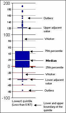
To construct a box plot, first, each observation (community, in this case) is sorted from the smallest to largest in terms of the value of the indicator (or variable) along the horizontal axis. Quintiles are formed by placing the smallest one-fifth of the observations into the first quintile, the next one-fifth of the observations into the second quintile, and so on.

Thus, each quintile contains one-fifth of the observations, as classified by the variable along the horizontal axis. The values in brackets along the horizontal axis indicate the lower and upper range of the values for observations included in a given quintile (i.e., in terms of the value of the indicator or variable measured along the horizontal axis).

Secondly, the boxes, whiskers and dots in each quintile (in each column) report the values of the outcome indicator (or variable) as measured on the vertical axis. In this bulletin, the outcome variable is the percent change in total population of each community from 1981 to 2006.

The central line within each box indicates the value of the Outcome indicator (or variable, as read along the vertical axis) for the median observation (community) within the given quintile. The median (or 50th percentile) is the value for which one-half of the observations have a higher value and one-half of the observations have a lower value. For boxes that are symmetric, the central line is likely to be similar to the average value of the outcome variable within the given quintile.

The central box shows the range in the values of the outcome variable (along the vertical axis) for the central 50% of observations (communities) when measured in terms of the values along the vertical axis. Within the box, there are 25% of the observations above the central line and 25% of the observations below the central line. The distance between the 25th and 75th percentiles (i.e. the height of the box, called the inter-quartile range) indicates the size of the spread in the outcome (vertical axis) variable that covers the "middle half" of the data. Boxes with a greater height means that a wider range of outcomes must be considered to include 50% of the observations.

The whiskers indicate the range or distribution of the outcome variable (as measured along the vertical axis) of the observations (communities) within the dataset that are outside of the middle half (i.e. outside those captured by the box). The whiskers extend upward from the top edge of the box and downward from the bottom edge of the box until each reaches a data point that is no further than 1.5 times the inter-quartile range (the height of the box), respectively. The terminal point of each whisker is called the upper or lower adjacent value, depending on which whisker is involved. Any data points above or below the end of the whiskers are considered outliers since these few communities have a rate of population growth that is unusually high or low relative to most of the communities in the data set (which are covered by the box and its whiskers). So, the whiskers represent the "outer" half of the data.

Box 4 Methods: a population growth model for Canadian communities

A regression model is used to determine the factors associated with community population change over the period 1981 to 2006. The population change between 1981 and 2006 is explained as a function of community and regional characteristics in 1981. The model is estimated in log-linear form, meaning that all variables are expressed either as logarithms or as dummy variables. The dependent variable is the logarithm of population change (where the change is computed as the ratio between population in 2006 and 1981); the explanatory variables are the logarithm of the level of each variable for the year 1981.

This functional form fits some of the data characteristics well, such as non-linear relationships and skewed distributions. Most importantly, the regression coefficients for the logarithmic variables can be interpreted as an elasticity, that is, the coefficient is the estimated percent change in the dependent variable due to a 1 percent change in the independent variable. The disadvantage, however, is the presence of zero values for some explanatory variables, for which logarithmic transformation is not possible. Although a relatively small proportion of observations have a zero for some variables (see Appendix Table A2), their presence needed to be addressed. For practical purposes, a dummy variable was used to assess the independent effect of presence/absence of the attribute. Then, the coefficient on the variable in each case was interpreted as the elasticity, given that the factor was present in the community. Following these considerations, the structure of the model that was estimated is as follows:

Description

where, Sector, Agglom, SocioEco and Demo, represent a set of variables capturing employment structure, agglomeration, socio-economic and demographic characteristics, respectively. The superscript c indicates community level variables, the superscript r indicates regional level variables (computed as spatial lag variables), while D indicates dummy variables introduced to account for zero values in the data before the logarithmic transformation. Appendix Table A1 reports the exact definition of each variable used in the model while Appendix Table A2 shows the descriptive statistics at the community level.

This model is estimated for the entire sample of communities (2,382 CCSs) and for rural and urban sub-samples (Appendix Table A3) and five macro-regional sub-samples (Appendix Table A4). Finally, results are also presented for a weighted regression, using community population in 1981 as weights, and including provincial and macro-regional dummies (Appendix Table A5). The measures of fit indicate that the model has a good explanatory power, with a R² ranging from 0.51 to 0.73; hence, depending on the sample used, up to 73% of the observed variation in population growth is explained by the model. A similar model was also estimated for the period 1981 to 2001 using alternative specifications (linear form, and alternative variable definitions). The main findings remain substantially unchanged. These results are available from the author upon request.

Interpretation. In the specific case of this dataset, given that the mean of the independent variable is closer to zero (it is 10.71), the coefficient on an independent variable can be interpreted as the expected "percentage point change" in the population growth rate, due to a 1% change in the independent variable. A detailed explanation follows.

The coefficients on an independent variable in a double-log equation (i.e. when the dependent variable and the independent variables are each entered as logarithms of the variable in question) are interpreted as – if the independent variable was different by 1%, then the percent difference in the dependent variable is given by the value of the coefficient.

For example, in our results for all communities (Appendix Table A3), the coefficient for the variable measuring the level of regional educational attainment is 0.165. Thus, an increase in the regional educational attainment level of 1% would increase the dependent variable by 0.165%. Our dependent variable is the ratio of the population in 2006 divided by the population level in 1981. For example, a population decline of 15% gives a ratio of 0.85 and a population increase of 15% gives a ratio of 1.15. Thus, the regional educational attainment coefficient of 0.165 means that the ratio of 2006/1981 population would be higher by 0.165% if regional education attainment was higher by 1%. As noted in Appendix Table A2, the percent change in population for the average community is 10.71% -- which, as a ratio of 1.1071, was our dependent variable. With a 1% increase in the level of regional educational attainment, our coefficient of 0.165 indicates that this ratio will increase by 0.165%. The new ratio would be 1.1071 plus (1.1071*(0.165/100)) = 1.108927. Thus, the percent change in population in this scenario would be 10.89%. The increase in the rate of population change is (10.89 – 10.71) = 0.18 percentage points. This value is approximately equal to the coefficient of 0.165.

The short story of the long explanation above is that since the mean of the independent variable is "close" to zero, the coefficient on an independent variable can be interpreted as the expected "percentage point difference" in the population growth rate due to a 1% change in the independent variable.

The coefficient on a dummy variable can be transformed to compute the shift in the dependent variable when the attribute is present. For example, if the coefficient (β) of a dummy is 0.2, when the dummy takes the value 1 the dependent variable is (Exp(β)-1) = 0.22 percentage points larger than otherwise.

Regional indicators. While the community variables are variables at the CCS level, the regional variables are spatial lags computed from the corresponding CCS indicators and a matrix of distances between each pair of communities. Specifically, spatial lags are computed as distance weighted averages of the values reported by neighbouring communities, where the weights are the inverse of the squared distance between community geographic centroids. A threshold distance of 1,000 kilometres is used to limit spatial interaction and beyond this threshold, the interaction is assumed to be zero (for details, see Alasia et al. 2007). The regional variable includes all the values of the neighbouring communities but not the value of the community itself. This approach mitigates the effect of any imposed administrative geography in defining the regional dimension, while at the same time accounts for the fact that regional interactions decay as distance increases. Thus, the role of neighbouring communities declines as one gets further and further from the observed community.