
In sickness and in health: The association between health and household income

Archived Content
Information identified as archived is provided for reference, research or recordkeeping purposes. It is not subject to the Government of Canada Web Standards and has not been altered or updated since it was archived. Please "contact us" to request a format other than those available.
By Steve Martin
Income Statistics Division,
Statistics Canada
Skip to text
Text begins
Abstract
This study examines the association between self-reported health and spouse-pair labour-market income using data from the Longitudinal and International Study of Adults. To explore the channels through which health associates with individual labour-market income, the association between health and spouse-pair income is further broken down into the association between health and the probability of working, hours worked, and hourly wage, both for an individual’s health and their spouse’s health.
Keywords: Health, household income, human capital, Longitudinal and International Study of Adults.
1. Introduction
Poor health is costly for society. Addressing both the acute effects of poor health in the short-term, and the more detrimental effects of poor health in the long-term, requires the use of scarce resources and highly skilled labour.Note 1 Beyond this direct cost, however, human capital theory stipulates that an individual’s health is positively correlated with their functioning as an economic unit—a healthy individual can both supply more labour and supply higher quality labour through increased productivity. Bad health outcomes are then costly for society, not only because of the direct costs associated with treating poor health, but also because of the indirect costs stemming from changes in individuals’ labour supply.Note 2
In addition to having a potentially large impact on the societal allocation of resources, poor health can have a significant impact on a household’s economic well-being if it results in reduced household income. This can lead to financial hardships, compounding lower income with increased medical or other associated expenses. There can also be intra-household spillovers from poor health resulting in a change in the labour-market activity of other working-age members of the household that further influence household income. For example, if an individual becomes chronically ill and drops out of the labour force, their spouse may work fewer hours to help care for them, which would in turn further reduce household income.
This study uses data from the Longitudinal and International Study of Adults (LISA) to analyze the association between health and household income. In order to focus on the labour-market outcomes associated with poor health and the intra-household spillovers that can come from poor health outcomes, the study restricts attention to spouse-pairs and considers the association between individual health and spouse-pair labour-market income—the sum of labour-market income for both members of a couple—rather than total household income. While there are non-labour market channels through which health can affect household income (e.g., by affecting discount rates), spouse-pair income is nonetheless a major component of household income for couples. In contrast to much of the existing literature that examines the association between health and a particular labour-market outcome for an individual, examining spouse-pair income allows the study to focus on the association between broader household income and health, and the labour-market channels through which this association propagates.
Using data on both self-reported general health and self-report mental health, as well as self-reported labour-market outcomes and linked tax records, the association between spouse-pair labour-market income and health is further decomposed into an employment effect reflecting the association between health and the probability of employment, an hours worked effect reflecting the association between health and the number of hours worked, and a wage effect reflecting the association between health and hourly wages. This is done for both for an individual’s health and their spouse’s health in order to examine intra-household spillovers from changes in health that correlate with spousal labour-market outcomes.
There is a large literature that examines the impact of self-reported health on particular labour-market outcomes, such as number of hours worked or hourly wages, with recent analyses exploiting panel datasets (e.g., Contoyannis and Rice, 2001; Cai, 2009; Han et al., 2009; Jäckle and Himmler, 2010).Note 3 Most of these studies use large socio-economic panel surveys (e.g., German Socio-Economic Panel, British Household Panel Survey) to examine the relationship between a measure of self-reported health and some labour-market outcome. While these analyses offer insights into the association between health and particular labour-market outcomes, they are silent on the size of intra-household spillovers from health, and how an individual’s health in turn relates to household income. Older studies find that men’s health can have an impact on the labour supply of female spouses (Chirikos, 1993).
Furthermore, very little research uses Canadian data, with no analyses using the LISA. The closest studies using Canadian datasets are those by Jeon (2014) and Jeon and Pohl (2016), who examine the impact of cancer diagnosis on both employment and household income using a panel dataset, and particularly Uppal (2009), who evaluates the assocation between self-reported health (both physical and mental) and hours worked for an individual.Note 4
In terms of results for this study, there is a strong negative association between both general and mental health and spouse-pair labour-market income, for both men and women. Spouse-pair income is particularly sensitive to mental health for men and general health for women. Poor mental health for men is associated with a $19,000 lower spouse-pair income, relative to those who do not have poor mental health. For women, having poor general health is associated with having a $28,000 lower spouse-pair income, relative to those who do not have poor general health. While the association between men’s mental health and spouse-pair income is almost entirely explained by the association between mental health and individual labour-market income for men, there are significant intra-household spillovers associated with women’s general health that are reflected in their spouse’s labour-market income. Put differently, the study finds a statistical association between women’s general health and their male spouse’s labour supply that does not operate in the other direction (i.e., when it is the male partner that has poor health). It should be underscored that this result is not demonstrated to be causal; poor health for women does not necessarily cause their male partners to reduce their labour supply. However, it suggests that women with poor general health may face an additional disadvantage, as their spouses tend to have diminished labour supply.
Decomposing these associations, men who have poor mental health earn less in the labour market because they are less likely to work, relative to those who do not have poor mental health. Of those who do work, men with poor mental health receive smaller hourly wages. Women with poor general health earn less because they are less likely to work, with those who do work spending fewer hours per week at work. In addition, women with poor general health have spouses with signficantly lower hourly wages. These channels of association accumulate to make spouse-pair income particularily sensitive to women’s health.
2. Data
The data used for this study come from the second wave of the Longitudinal and International Study of Adults (LISA), conducted in 2014. The LISA is a biennial Canadian household survey that follows the same individuals over time, asking a variety of socio-economic questions. It targets individuals living in the ten provinces as of 2012, and is administered to all members of the household that are 15 years of age and older. The full description of the target population for the LISA can be found in Statistics Canada (2015).
For the purpose of this study, the LISA collects information on self-reported general and mental health for all respondents. Both general and mental health are measured using a five point scale—poor, fair, good, very good, and excellent. The LISA also asks the Kessler K10 set of questions on mental distress (Kessler et al., 2002), which can be used as an alternate measure of mental health.Note 5 For labour-market outcomes, the LISA collects self-reported information on employment, average hours worked per week, and hourly wages, as well as a variety of other socio-economic variables such as age, education, and household composition. To avoid issues associated with absenteeism at work stemming from poor health, whether an individual worked in the week of the interview or not is used to measure employment.
| Labour-market variables | Men | Women |
|---|---|---|
| dollars | ||
| Spouse-pair income | 104,800 | 103,800 |
| Individual income | 67,600 | 36,500 |
| Hourly wage | 31.8 | 25.3 |
| hours | ||
| Hours worked per week | 45.1 | 37.5 |
| percent | ||
| Employment rate | 86.5 | 75.9 |
| Self-reported general health | ||
| Good/very good/excellent | 93.1 | 93.9 |
| Fair/poor | 6.9 | 6.1 |
| Self-reported mental health | ||
| Good/very good/excellent | 95.9 | 95.6 |
| Fair/poor | 4.1 | 4.4 |
| Kessler K10 | ||
| Below 20 | 93.0 | 90.4 |
| Above 20 | 7.0 | 9.6 |
| N. Obs. | 2,820 | 2,814 |
|
Note: All estimates use sample weights. Source: Statistics Canada, Longitudinal and International Study of Adults (2014). |
||
The LISA also links with administrative tax data, which gives a measure of annual before-tax labour-market income at the individual level. Spouse-pair labour-market income is simply the sum of both member’s before tax labour-market income.Note 6 In this study, income refers to before-tax income from the previous tax year, whereas employment, hours worked, and wages are measured in the week of the interview. Interviews occur near the start of the calendar year, so there is minimal lag between measuring annual income from tax data and the other labour-market variables.
In order to focus on the labour-market implications of poor health and capture any intra-household spillovers from an individual’s health, attention is restricted to spouse-pairs where both members are between 18 and 64 years of age, not enrolled in an education program, and not self-employed. The result is a sample of 5,634 spouse pairs. Table 1 provides basic summary statistics. The vast majority of spouse-pairs are of the opposite sex, so that any association between spousal health and an individual’s labour-market outcomes can be broadly interpreted as coming from a member of the opposite sex.
Before presenting the model used to analyze the data, it is useful to examine the association between health and spouse-pair income graphically. Charts 1 and 2 show how spouse-pair labour-market income relates to both general and mental health for men and women, respectively. For men, having either poor general health or poor mental health is associated with a roughly $30,000 drop in spouse-pair income compared to those with good to excellent health. Most of this drop is accounted for by a reduction in individual labour-market income, with only a small decrease in spousal labour-market income.
Compared to men, women’s general health has a stronger association with spouse-pair income—poor health is associated with a $37,000 drop in spouse-pair income relative to those that have good to excellent health (Chart 2). Only half of this association, however, is related to lower individual labour-market income for women. The other half comes from lower spousal labour-market income, suggesting that there may be important intra-household spillovers from women’s health that are reflected in poorer spousal labour-market outcomes.
Compared to men, women’s mental health is not as strongly associated with spouse-pair income—having poor mental health is associated with a $22,000 lower spouse-pair income, compared to $29,000 less for men. As was the case for men, most of this association is accounted for by reduced individual labour-market income, with spousal income being only slightly lower.
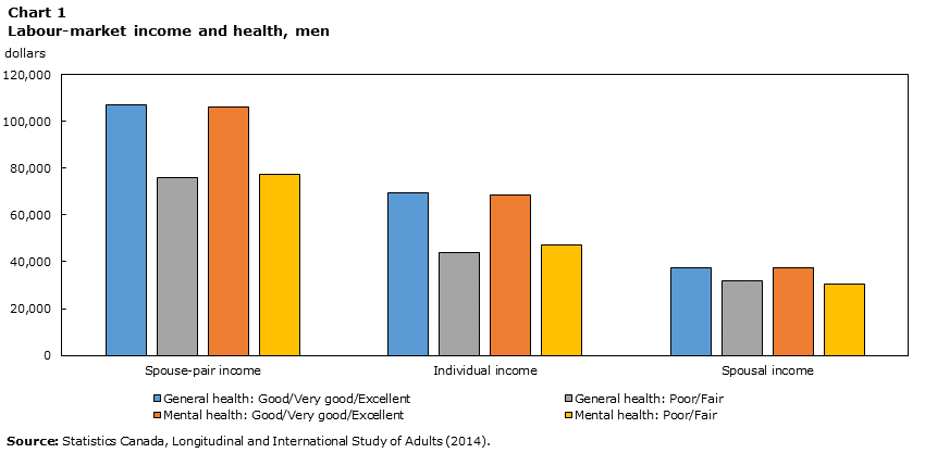
Data table for Chart 1
| Spouse-pair income | Individual income | Spousal income | |
|---|---|---|---|
| dollars | |||
| General health: Good/Very good/Excellent | 107,000 | 69,400 | 37,600 |
| General health: Poor/Fair | 75,800 | 44,000 | 31,800 |
| Mental health: Good/Very good/Excellent | 106,000 | 68,500 | 37,500 |
| Mental health: Poor/Fair | 77,500 | 47,100 | 30,400 |
| Source: Statistics Canada, Longitudinal and International Study of Adults (2014). | |||
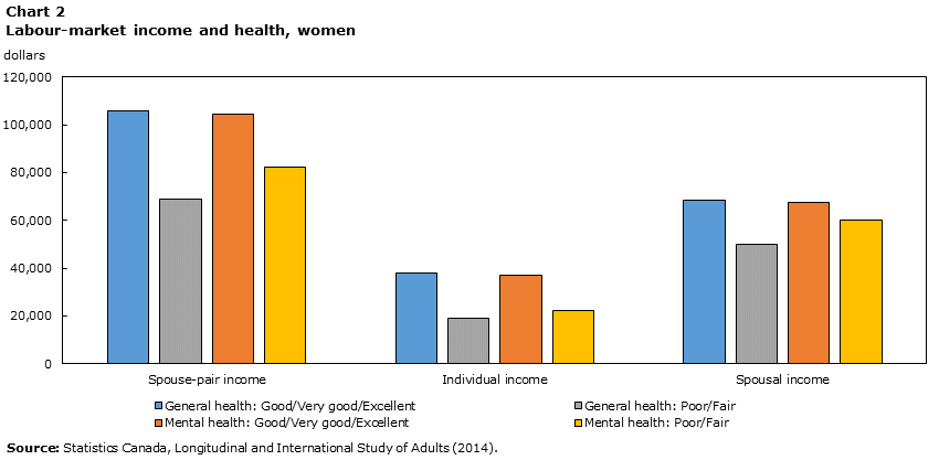
Data table for Chart 2
| Spouse-pair income | Individual income | Spousal income | |
|---|---|---|---|
| dollars | |||
| General health: Good/Very good/Excellent | 106,000 | 37,700 | 68,400 |
| General health: Poor/Fair | 68,900 | 19,100 | 49,800 |
| Mental health: Good/Very good/Excellent | 104,700 | 37,200 | 67,600 |
| Mental health: Poor/Fair | 82,500 | 22,400 | 60,100 |
| Source: Statistics Canada, Longitudinal and International Study of Adults (2014). | |||
3. Empirical model
In order to understand the channels through which health associates with spouse-pair income, the study examines how health—both for an individual and their spouse—associates with an individual’s labour-market income. A change in an individual’s labour-market income resulting from a change in health (either individual or spousal health) can be decomposed into three separate effects; see the Appendix for details.
- i) The employment effect that results from a change in the probability of employment from a change in health.
- ii) The hours worked effect that results from a change in the average number of hours worked from a change in health, conditional on working.
- iii) The wage effect that results from a change in the hourly wage from a change in health, conditional on working.
To estimate the association between health and household income, and operationalize the income decomposition presented above, a series of linear regression models are estimated, for both men and women, of the form
Here yi is a labour-market outcome for individual i, is an individual’s own self-reported health status, is an individual’s spouse’s self-reported health status, and Xi is a vector of observable covariates. Covariates include five equal-sized bins for age (for individuals and spouses); dummies for education—no post-secondary, post-secondary below the bachelors level, post-secondary at the bachelors level or above (for individuals and spouses); dummies for age of children (0-5, 6-17, 18-24); province dummies and a dummy for if the household is in a rural area; and a dummy for being born in Canada (for individuals and spouses).Note 7 These correspond closely to the controls found in existing research — e.g., Cai (2009), Uppal (2009), and Jäckle and Himmler (2010).
When the dependent variable yi equals labour-market income, the regression coefficient β gives the association between an individual’s health and their income, and γ gives the association between spousal health and an individual’s income. Setting yi equal to a dummy indicating employment, the number of hours worked, and the hourly wage in turn gives the employment effect, hours worked effect, and wage effect discussed above, both with respect to own health, β, and spousal health, γ.Note 8 As the vast majority of spouse-pair couples in the data are of the opposite sex, the spousal coefficient γ can broadly be interpreted as coming from a member of the opposite sex.
4. Results
Table 2 presents the model results for men. The left-most column shows the association between general health and mental health—both for an individual and their spouse—and spouse-pair labour-market income, analogous to chart 1. Looking at the first two rows, poor general health is associated with having $12,000 less in spouse-pair income relative to those with good to excellent general health, whereas poor mental health is associated with having $19,000 less in spouse-pair income relative to those with good to excellent mental health.
Moving from left to right across the table, the association between men’s health and spouse-pair income is almost entirely explained by the association between men’s health and individual income (second column). For general health, this association is driven primarily by a strong negative association between health and the probability of working (third column)—men with poor general health are 20 percentage points less likely to be employed compared to men with good to excellent general health. For men who are employed, there is little association between either the number of hours worked (fourth column) or the hourly wage (fifth column) and general health.
For mental health, a lower probability of working (third column) and a lower hourly wage (fifth column) contribute to the negative association with income. Men with poor mental health are 10 percentage points less likely to be employed, and those who are employed make $3 less per hour on average. This may explain why the association between labour-market income and mental health is so much larger than the association between labour-market income and general health. Poor mental health not only makes it less likely that an individual will work, but those that do work are less productive in the labour market.
| Spouse-pair income | Individual income | Employment | Hours worked | Hourly wage | |
|---|---|---|---|---|---|
| dollars | percentage points | hours | dollars | ||
| Individual health | |||||
| Self-reported general health | |||||
| Good/very good/excellent (ref.) | Note ...: not applicable | Note ...: not applicable | Note ...: not applicable | Note ...: not applicable | Note ...: not applicable |
| Fair/poor | -11,800Note * | -13,800Note * | -19.7Note * | 0.5 | 1.1 |
| Self-reported mental health | |||||
| Good/very good/excellent (ref.) | Note ...: not applicable | Note ...: not applicable | Note ...: not applicable | Note ...: not applicable | Note ...: not applicable |
| Fair/poor | -18,900Note * | -15,100Note * | -10.3Note * | -2.8 | -2.7Note * |
| Spousal health | |||||
| Self-reported general health | |||||
| Good/very good/excellent (ref.) | Note ...: not applicable | Note ...: not applicable | Note ...: not applicable | Note ...: not applicable | Note ...: not applicable |
| Fair/poor | -28,200Note * | -13,000Note * | -1.8 | 0.0 | -4.9Note * |
| Self-reported mental health | |||||
| Good/very good/excellent (ref.) | Note ...: not applicable | Note ...: not applicable | Note ...: not applicable | Note ...: not applicable | Note ...: not applicable |
| Fair/poor | -10,600Note * | -2,300 | 1.3 | -0.5 | -1.3 |
| N. Obs. | 2,820 | 2,336 | |||
... not applicable
Source: Statistics Canada, Longitudinal and International Study of Adults (2014). |
|||||
Examining the last two rows of the table, a spouse with poor general health is associated with a $28,000 lower spouse-pair income, well over double the size of the association between men’s own general health and spouse-pair income. Moving from left to right across the columns of the table, about half of this association is explained by smaller labour-market income for men (second column)—poor spousal health is associated with their male partner’s labour-market income being $13,000 lower. This smaller labour-market income in turn comes primarily from a $5 lower average hourly wage for men (fifth column), suggesting that there are large intra-household spillovers associated with women’s health that are negatively reflected in their male partner’s labour-market productivity. In contrast, while spousal mental health is negatively associated with spouse-pair income (an $11,000 reduction in spouse-pair income), there are no significant intra-household spillovers from spousal mental health that are seen in men’s labour-market income.
Analogous to table 2, table 3 gives the model results for women. As the vast majority of spouse-pairs are of the opposite sex, the first column in table 3 is nearly identical to the first column in table 2. Working across the first two rows, women’s poor general health has a strong, negative association with spouse-pair income—having poor general health is associated with $28,000 less in spouse-pair income. Consistent with table 2, about half of this association is accounted for by the association between individual income and general health (second column). This is in turn is driven by both a lower probability of working and fewer hours worked. Relative to those with good to excellent general health, women having poor health are 22 percentage points less likely to be employed (third column) and those who are employed work 3 hours less per week on average (fourth column).
| Spouse-pair income | Individual income | Employment | Hours worked | Hourly wage | |
|---|---|---|---|---|---|
| dollars | percentage points | hours | dollars | ||
| Individual health | |||||
| Self-reported general health | |||||
| Good/very good/excellent (ref.) | Note ...: not applicable | Note ...: not applicable | Note ...: not applicable | Note ...: not applicable | Note ...: not applicable |
| Fair/poor | -27,800Note * | -14,800Note * | -22.1Note * | -3.1Note * | -1.3 |
| Self-reported mental health | |||||
| Good/very good/excellent (ref.) | Note ...: not applicable | Note ...: not applicable | Note ...: not applicable | Note ...: not applicable | Note ...: not applicable |
| Fair/poor | -10,500Note * | -8,100Note * | -13.5Note * | 0.3 | -1.0 |
| Spousal health | |||||
| Self-reported general health | |||||
| Good/very good/excellent (ref.) | Note ...: not applicable | Note ...: not applicable | Note ...: not applicable | Note ...: not applicable | Note ...: not applicable |
| Fair/poor | -11,900Note * | 2,500 | -0.8 | -1.7 | -0.1 |
| Self-reported mental health | |||||
| Good/very good/excellent (ref.) | Note ...: not applicable | Note ...: not applicable | Note ...: not applicable | Note ...: not applicable | Note ...: not applicable |
| Fair/poor | -19,000Note * | -3,600 | -2.5 | -1.0 | -2.1 |
| N. Obs. | 2,814 | 2,074 | |||
... not applicable
Source: Statistics Canada, Longitudinal and International Study of Adults (2014). |
|||||
As for mental health, women having poor mental health is associated with an $11,000 lower spouse-pair income, with this association almost entirely explained by the association between mental health and individual income (second column). This lower individual income is in turn explained primarily by a lower probably of working—women with poor mental health are 14 percentage points less likely to work than those reporting good to excellent mental health (third column).
Moving to the last two rows of the table, spousal health—especially spousal mental health—is strongly associated with spouse-pair income. Consistent with table 1, however, there is very little association between women’s labour-market income and spousal health. The contribution of men’s health to spouse-pair income is almost entirely explained by the association between men’s health and men’s labour-market income.
Tables 4 and 5 are analogous to tables 3 and 4, except that the previous measure of mental health is now replaced by the Kessler K10 measure of psychological distress. The regression coefficients for general health, both for an individual and their spouse, are virtually unchanged across the columns of both tables. The coefficients for mental health are smaller in both tables, particularly for women’s mental health, although the main qualitative insights from tables 2 and 3 remain unchanged.
| Spouse-pair income | Individual income | Employment | Hours worked | Hourly wage | |
|---|---|---|---|---|---|
| dollars | percentage points | hours | dollars | ||
| Individual health | |||||
| Self-reported general health | |||||
| Good/very good/excellent (ref.) | Note ...: not applicable | Note ...: not applicable | Note ...: not applicable | Note ...: not applicable | Note ...: not applicable |
| Fair/poor | -13,500Note * | -14,100Note * | -19.3Note * | 0.2 | 0.9 |
| Self-reported mental health | |||||
| K10 below 20 (ref.) | Note ...: not applicable | Note ...: not applicable | Note ...: not applicable | Note ...: not applicable | Note ...: not applicable |
| K10 above 20 | -14,600Note * | -16,300Note * | -13.5Note * | -1.1 | -2.6Note * |
| Spousal health | |||||
| Self-reported general health | |||||
| Good/very good/excellent (ref.) | Note ...: not applicable | Note ...: not applicable | Note ...: not applicable | Note ...: not applicable | Note ...: not applicable |
| Fair/poor | -29,600Note * | -13,300Note * | -0.9 | -0.2 | -5.8Note * |
| Self-reported mental health | |||||
| K10 below 20 (ref.) | Note ...: not applicable | Note ...: not applicable | Note ...: not applicable | Note ...: not applicable | Note ...: not applicable |
| K10 above 20 | -3,500 | -1,700 | -3.5 | 0.4 | 1.9 |
| N. Obs. | 2,820 | 2,336 | |||
... not applicable
Source: Statistics Canada, Longitudinal and International Study of Adults (2014). |
|||||
5. Conclusions
This study examines the association between self-reported general and mental health and spouse-pair labour-market income for couples using data from the LISA. Focusing on labour-market income rather than total income allows the analysis to examine the labour-market channels through which health associates with income, while focusing on spouse-pairs allows the analysis to examine intra-household spillovers in labour-market outcomes from poor self-reported health. This offers a novel perspective on the association between health and household income using a previously unexploited dataset, assessing both the channels through which health associates with income and extent to which intra-household spillovers in labour-market activity from health are reflected in household income.
The results show that spouse-pair income is strongly associated with both men’s and women’s self-reported health. For men, the association between mental health and income is particularly strong, whereas for women it is the association between general health and income that is stronger. While the association between men’s health and spouse-pair income is almost entirely explained by the association between men’s health and individual income, for women about half of the association between general health and spouse-pair income is explained by lower income for their male partners. This latter finding suggests that there may be important intra-household spillovers from women’s health that are associated with their partner’s labour supply.
While the LISA is a panel dataset, the analysis is entirely cross-sectional in nature as the panel is still short. However, the longitudinal aspect of the LISA offers interesting opportunities for future research, as future waves of the survey will allow for the estimation of fixed-effects models that control for time-invariant individual heterogeneity. This is practically relevant when using self-reported health data, as this offers a means to control for individual-specific reference points when reporting health, as well as historical health that can be correlated with both current health and current labour-market outcomes.
| Spouse-pair income | Individual income | Employment | Hours worked | Hourly wage | |
|---|---|---|---|---|---|
| dollars | percentage points | hours | dollars | ||
| Individual health | |||||
| Self-reported general health | |||||
| Good/very good/excellent (ref.) | Note ...: not applicable | Note ...: not applicable | Note ...: not applicable | Note ...: not applicable | Note ...: not applicable |
| Fair/poor | -28,300Note * | -15,300Note * | -22.9Note * | -3.0Note * | -1.8 |
| Self-reported mental health | |||||
| K10 below 20 (ref.) | Note ...: not applicable | Note ...: not applicable | Note ...: not applicable | Note ...: not applicable | Note ...: not applicable |
| K10 above 20 | -6,400 | -4,200Note * | -6.8Note * | -0.4 | 1.1 |
| Spousal health | |||||
| Self-reported general health | |||||
| Good/very good/excellent (ref.) | Note ...: not applicable | Note ...: not applicable | Note ...: not applicable | Note ...: not applicable | Note ...: not applicable |
| Fair/poor | -12,900Note * | 1,700 | -1.8 | -2.0 | -0.1 |
| Self-reported mental health | |||||
| K10 below 20 (ref.) | Note ...: not applicable | Note ...: not applicable | Note ...: not applicable | Note ...: not applicable | Note ...: not applicable |
| K10 above 20 | -17,700Note * | -1,200 | -0.2 | 1.0 | -2.6Note * |
| N. Obs. | 2,814 | 2,074 | |||
... not applicable
Source: Statistics Canada, Longitudinal and International Study of Adults (2014). |
|||||
Appendix
This appendix shows the details of the income decomposition used in section 3. To fix notation, let w denote the hourly wage rate, l the number of hours worked, and e an indicator of employment. Conditional on a vector of covariates x and health, denoted by h, expected labour-market income is
In order to lighten notation, in what follows the conditioning vector x is omitted; all expectations should be interpreted as conditional on x. From the above expression, it follows that a change in health status from h to h' is given by
Since , after some manipulation this expression can be written as
Under the assumption that is constant the residual effect disappears, so that
This constant covariance assumption is standard for system equation models; see Greene (2011, Chapter 10) for details. Importantly, this assumption does not imply that wages and hours of work are uncorrelated; rather, the correlation does not change with health status after controlling for key demographic variables. If this assumption does not hold, then the residual covariance term does not disappear. While the decomposition used in section 3 is still valid in this case, it is no longer an exact decomposition.
Under the usual assumptions of the linear regression model, the employment effect, the hours worked effect, and the wage effect can be estimated respectively by regressing an employment indicator, hours worked, and hourly wage on health status (and a vector of covariates).
References
Bound, J. (1991). Self-reported versus objective measures of health in retirement models. Journal of Human Resources, 26(1), 106-138.
Cai, L. (2009). Effects of Health on Wages of Australian Men. Economic Record, 85(270), 290-306.
Cai, L. (2010). The relationship between health and labour force participation: Evidence from a panel data simultaneous equation model. Labour Economics, 77, 77-90.
Chirikos, T. N. (1993). The Relationship Between Health and Labour Market Status. Annual Review of Public Health, 14, 293-312.
Contoyannis, P., and Rice, N. (2001). The Impact of Health on Wages: Evidence from the British Household Panel Survey. Empirical Economics, 26, 599-622.
Greene, W. H. (2011). Econometric Analysis (7th ed.). Pearson.
Han, E., Norton, E. C., and Stearns, S. C. (2009). Weight and Wages: Fat Versus Lean Paychecks. Health Economics, 18, 535-548.
Jäckle, R., and Himmler, O. (2010). Health and Wages: Panel Data Estimates Considering Selection and Endogeneity. Journal of Human Resources, 45(2), 364-406.
Jeon, S.-H. (2014). The Effects of Cancer on Employment and Earnings of Cancer Survivors. Analytical Studies Branch Research Paper Series, Statistics Canada.
Jeon, S.-H., and Pohl, R. V. (2016). Health and Work in the Family: Evidence from Spouses’ Cancer Diagnoses. Analytical Studies Branch Research Paper Series, Statistics Canada.
Kessler, R. C., Andrews, G., Colpe, L. J., and Hiripi, E. (2002). Short screening scales to monitor population prevalences and trends in non-specific psychological distress. Psychological Medicine, 32(6), 959-976.
Lundberg, O., and Manderbacka, K. (1996). Assessing reliability of a measure of self-rated health. Scandinavian Journal of Social Medicine, 24(3), 218-224.
Public Health Agency of Canada. (2014). Economic Burden of Illness in Canada, 2005-2008.
Sharpe, A., and Murray, A. (2011). State of Evidence on Health as a Determinant of Productivity. Centre for the Study of Living Standards.
Statistics Canada. (2015, December 7). Longitudinal and International Study of Adults (LISA).
Uppal, S. (2009). Health and Employment. Perspectives, Statistics Canada.
- Date modified: