Methods for Constructing Life Tables for Canada, Provinces and Territories

Report prepared by Demography Division^{Note 1}

Introduction

Life tables are used to compute life expectancy at birth and at different ages, but they are also used to compute many other indicators: death probabilities, probabilities of survival between two ages, number of years of life lived and the number of survivors at different ages. The construction of a life table makes it possible to summarize mortality within a population at a given time (period life table) or within a cohort (cohort life table). Accordingly, life tables meet many statistical needs, particularly in the fields of health, epidemiology, and actuarial science, and facilitate comparisons between regions or cohorts.

Since 1939, Statistics Canada has disseminated life tables, both complete (by single years of age) and abridged (by five-year age groups) for Canada, the provinces and territories. The methodology on which these period life tables are based has also been revised occasionally, following advances in the field of mortality studies. A major revision was undertaken in 2013 of the methodology described in this document to take into account current methods for constructing life tables. This revision was also an opportunity to incorporate the work conducted in the context of the development of the Human Mortality Database (HMD),^{Note 2} a database aiming to facilitate comparisons of mortality data between a large number of countries and regions, including Canada.^{Note 3} While differences remain between the two methods, the increased consistency between the methodology used by Statistics Canada and that of the HMD offers many advantages, especially for analysis and demographic projections.

This methodology document is divided into three parts. The first part presents data sources and steps for the construction of complete life tables. These tables are calculated for Canada and all of the provinces except Prince Edward Island. Complete life tables have the advantage of being more detailed than abridged tables, especially for older ages, where the decline in mortality has been concentrated for some years now.

The second part presents data sources and steps for the construction of the abridged life tables used for Prince Edward Island, Yukon, the Northwest Territories and Nunavut. Abridged life tables must be used when population sizes and death counts are too small to calculate complete life tables accurately.

Methodology for complete life tables

Using the revised methodology of Statistics Canada’s life tables, the construction of such tables is a seven-step process:

Step 1: Calculation of observed mortality rates for the ages 5 to 109 and for the open age group of 110 years and over;
Step 2: Modelling of observed mortality rates for ages 95 to 109 and for the open age group of 110 years and over;
Step 3: Calculation of death probabilities for ages 5 to the open age group of 110 years and over;
Step 4: Calculation of death probabilities for ages 0 to 4;
Step 5: Smoothing of death probabilities for ages 1 to 94;
Step 6: Calculation of the elements of the life table;
Step 7: Calculation of the margins of error for death probabilities and life expectancy.

Input data

Two data sources are used to construct complete life tables: Statistics Canada’s Vital Statistics and Demographic Estimates Program.

More specifically, for a given sex and region, the following four data sets are required to calculate a complete life table for a period extending from calendar year α-1 to year α+1:

• Observed number of deaths by year of age (from 5 to 109 years and for the open age group of 110 years and over) for calendar years (January 1 to December 31) α-1, α and α+1 (source: Vital Statistics);
• Observed number of deaths by year of age (from 0 to 4 years) and year of birth for calendar years α-1, α and α+1 (source: Vital Statistics);
• Population estimates on July 1 by age (from 5 to 110 years) for calendar years α-1, α and α+1 (source: Demographic Estimates Program);^{Note 4}
• Population estimates on January 1 by age (from 0 to 4 years) for calendar years α-1, α, α+1 and α+2 (source: Demographic Estimates Program).

In general, the input data on deaths by age and sex from Canadian Vital Statistics are considered to be of very good quality (Bourbeau and Lebel 2000), even between 80 and 100 years of age (Beaudry-Godin 2010). Each year, there are very few deaths with unknown age or sex; any that exist are redistributed according to the known structure of observed deaths by age and sex. There are also few late registrations of deaths in Canada.

Similarly, Statistics Canada’s population estimates are considered to be of very good quality. These estimates, used in the context of the Federal-Provincial Fiscal Arrangements Act, are based on the last available census, are adjusted for census net undercoverage and take into account demographic events since the last available census, by age and sex. Most often, postcensal population estimates are used to compute the life tables in a timely fashion.

Estimating mortality at 100 years and over presents a challenge, since population sizes and observed death counts are lower and records are more subject to reporting errors. However, the use of a logistic model makes it possible to obtain a coherent series of mortality rates in old age, since this series is modelled.

Step 1: Calculation of observed mortality rates for ages 5 to 109 and for the open age group of 110 years and over

For each year of age x included between age 5 and the open age group of 110 years and over, the observed mortality rate is computed by taking the ratio of the sum of deaths during the three-year period to the sum of the populations in the middle of each of the three years of the three-year of the same period. By doing so, it allows differentials in the population growth rate of the three calendar years to be used in the calculation of the mortality rates.

More specifically:

$${}_{\text{n}}\text{M}{}_{\text{x}}=\frac{{\displaystyle \sum _{\text{t}=a-1}^{a+1}{\text{D}}_{\text{x,t}}}}{{\displaystyle \sum _{\text{t}=a-1}^{a+1}{\text{P}}_{\text{x,t}}}}$$

where ${}_{\text{n}}\text{M}{}_{\text{x}}$ is the observed mortality rate between ages x and x+n (in the case of complete tables, n = 1); ${\displaystyle \sum _{\text{t}=a-1}^{a+1}{\text{D}}_{\text{x,t}}}$ is the sum of deaths between ages x and x+n for calendar years $a-1$ , $a$ and $a+1$ of the reference period, and; ${\displaystyle \sum _{\text{t}=a-1}^{a+1}{\text{P}}_{\text{x,t}}}$ is the sum of the population counts estimated on July 1 between ages x and x+n for calendar years $a-1$ , $a$ and $a+1$ of the reference period.

In the case where, for a given age, no deaths are observed during the reference period, a mortality rate is imputed based on a geographic approach according to Table 1.

Table 1
Regions associated to the different provinces, for imputation

Step 2: Modelling of observed mortality rates for ages 95 to 109 and for the open age group of 110 years and over

From age 95 up to the open age group of 110 years and over, the mortality rates calculated in Step 1 can exhibit important variations due to the small number of deaths and persons exposed to the risk of dying. It can even happen that at some very old ages, often beyond age 105, it is impossible to calculate rates because of a lack of deaths or at-risk population, a situation that arises frequently where there are small populations.

In these circumstances, it is better to use a model for estimating old-age mortality rates, which can yield both a more accurate representation of the mortality pattern, and a complete series of rates up to the open age group of 110 years and over. Therefore, a simplified logistic model based on the work of Kannisto (1992) is used.^{Note 5} This model is adjusted by the maximum likelihood method, and it features an upper asymptote equal to one.

The model takes the following form:

$${\text{μ}}_{\text{x}}=\frac{{\text{αe}}^{\text{βx}}}{1+{\text{αe}}^{\text{βx}}}$$

where ${\text{μ}}_{\text{x}}$ is the mortality force (mortality hazard in continuous time) at age x, and; $\alpha$ and $\text{β}$ are the parameters to be estimated.

The parameter $\alpha$ corresponds roughly to the baseline mortality at age 0 and $\text{β}$ corresponds to the rate of increase (logistic) of mortality from one age to the next. Parameters $\alpha$ and $\text{β}$ are assumed to be positive, meaning that this condition is enforced as the model is estimated. The model is estimated by SAS software’s NLIN procedure,^{Note 6} and for optimization, the Newton method is used (SAS Institute Inc. 2008A). The modelled mortality rate between age x and x+n corresponds to:

$${}_{\text{n}}\widehat{\mathrm{M}}{}_{\text{x}}={\widehat{\mu }}_{\text{(x+n)/2}}$$

To ensure that the logistic model properly adjusts the observed old-age data, a minimum of 15 observed mortality rates between age 80 up to the open age group of 110 years and over, calculated in Step 1, must be computable (and not imputed) for estimating the model.

Step 3: Calculation of death probabilities for ages 5 to the open age group of 110 years and over

Steps 1 and 2 yield a series of mortality rates for ages 5 to 110. These mortality rates are then converted into death probabilities by the so-called actuarial method:

$${}_{\text{n}}\text{q}{}_{\text{x}}=\frac{2\cdot \text{n}\cdot {}_{\text{n}}\text{M}{}_{\text{x}}^{\text{*}}}{2+(\text{n}\cdot {}_{\text{n}}\text{M}{}_{\text{x}}^{\text{*}})}$$

where ${}_{\text{n}}\text{q}{}_{\text{x}}$ is the death probability between ages x and x+n, that is the probability that an individual aged x die before reaching age x+n ; n is the age interval (in the case of complete life tables, n = 1), and; ${}_{\text{n}}\text{M}{}_{\text{x}}^{\text{*}}$ is either the observed mortality rate ( ${}_{\text{n}}\text{M}{}_{\text{x}}$ ) between ages x and x+n for x comprised between 5 and 94 years or the modelled mortality rate ( ${}_{\text{n}}\widehat{\text{M}}{}_{\text{x}}$ ) for x comprised between 95 and 110 years.

Within the open age group of 110 years and over, the death probability takes the value of one.

Step 4: Calculation of death probabilities for ages 0 to 4

Between ages 0 and 4, death probabilities are estimated directly, since mortality at these ages has its own particular pattern. For example, between 0 and 1 year of age, deaths are not distributed uniformly over the year, but are instead concentrated in the first days of life.

Schematically, and for a given year α, the calculation of the death probability at age 0 (₁q₀), also called the infant mortality rate, is based on one minus a product of two ratios, the first representing the probability that a person of exact age x will survive to the end of the calendar year in which that person reaches age x, and the second representing the probability that a person living at the end of the calendar year in which he or she reaches age x will survive until the exact age of x+1.

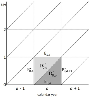
Thus, according to the Lexis diagram (Figure 1):

Figure 1
Lexis diagram

$${}_1\text{q}{}_0=1-\left(\frac{{\text{P}}_{0,a+1}^{*}}{{\text{E}}_{0,a}}\cdot \frac{{\text{E}}_{1,a}}{{\text{P}}_{0,a}^{*}}\right)$$

The value ${\text{E}}_{0,a}$ is obtained by adding to the population aged 0 on January 1 of year $a+1$ (value ${\text{P}}_{0,a+1}^{*}$ in Figure 1) the number of deaths at age 0 during year $a$ , among children born during that same year $a$ ( ${\text{D}}_{0,a}^{\prime }$ ). The value ${\text{E}}_{1,a}$ is obtained by subtracting from the population aged 0 on January 1 of year $a$ ( ${\text{P}}_{0,a}^{*}$ ) the number of deaths at age 0 during year $a$ , among children born during the previous year ( ${\text{D}}_{0,a}^{\prime \prime }$ ). Description for formula 12 step 4

By transposition and using three years for the calculations:

$${}_1\text{q}{}_0=1-\left(\frac{{\displaystyle \sum _{\text{t}=a-1}^{a+1}{\text{P}}_{0,\text{t}+1}}}{{\displaystyle \sum _{\text{t}=a-1}^{a+1}{\text{P}}_{0,\text{t}+1}}+{\displaystyle \sum _{\text{t}=a-1}^{a+1}{\text{D}}_{0,t}^{\prime }}}\cdot \frac{{\displaystyle \sum _{\text{t}=a-1}^{a+1}{\text{P}}_{0,\text{t}}}-{\displaystyle \sum _{\text{t}=a-1}^{a+1}{\text{D}}_{0,t}^{\prime \prime }}}{{\displaystyle \sum _{\text{t}=a-1}^{a+1}{\text{P}}_{0,\text{t}}}}\right)$$

where ${}_1\text{q}{}_0$ is the death probability at age 0; ${\displaystyle \sum _{\text{t}=a-1}^{a+1}{\text{P}}_{0,\text{t}+1}}$ is the sum of the population counts of age 0 estimated on January 1 of years $a$ , $a+1$ and $a+2$ , that is the last two years of the reference period and the year that follows; ${\displaystyle \sum _{\text{t}=a-1}^{a+1}{\text{D}}_{0,t}^{\prime }}$ is the sum of deaths at age 0 during the reference period, for children born in the same year as the year of their death; ${\displaystyle \sum _{\text{t}=a-1}^{a+1}{\text{P}}_{0,\text{t}}}$ is the sum of the population counts of age 0 estimated on January 1 during the reference period, and; ${\displaystyle \sum _{\text{t}=a-1}^{a+1}{\text{D}}_{0,t}^{\prime \prime }}$ is the sum of deaths at age 0 during the reference period, for children born during the year preceding the year of their death.

From ages 1 to 4 years, an equation following the same principle is used:

$${}_{\text{n}}\text{q}{}_{\text{x}}=1-\left(\frac{{\displaystyle \sum _{\text{t}=a-1}^{a+1}{\text{P}}_{\text{x,t+1}}}}{{\displaystyle \sum _{\text{t}=a-1}^{a+1}{\text{P}}_{\text{x,t}+1}}+{\displaystyle \sum _{\text{t}=a-1}^{a+1}{\text{D}}_{\mathrm{x},t}^{\prime }}}\cdot \frac{{\displaystyle \sum _{\text{t}=a-1}^{a+1}{\text{P}}_{\text{x,t}}}-{\displaystyle \sum _{\text{t}=a-1}^{a+1}{\text{D}}_{\mathrm{x},t}^{\prime \prime }}}{{\displaystyle \sum _{\text{t}=a-1}^{a+1}{\text{P}}_{\text{x,t}}}}\right)$$

When, for a given age between 1 and 4 years, no death is observed during the reference period, a death probability will be interpolated for this age in Step 5, when death probabilities are smoothed.

Step 5: Smoothing of death probabilities for ages 1 to 94

In steps 3 and 4, a complete series of death probabilities was computed for ages 0 to 110 years. However, between ages 1 and 94, these probabilities can exhibit an irregular pattern over time, especially for regions with small populations. To ensure that death probabilities evolve consistently from one age to another and to estimate, if needed, missing probabilities between ages 1 and 4, smoothing is applied using B-splines. This smoothing is applied to death probabilities from 0 to 109 years of age, to ensure a harmonious link between smoothing by means of B-splines and the model for estimating old-age mortality (Step 2).^{Note 7}

The B-spline smoothing technique has the advantage of being flexible, that is, to provide users many options to fit the data in the best way possible. Since B-splines, just like any other splines, are constructed using piecewise polynomial functions joined together, it is appropriate to choose various positions on the horizontal axis–or knots–where these junctions occur. The greater the number of knots, the better the smoothed curve fits the original curve of death probabilities by age; conversely, a small number of knots provides more power to the smoothing. As a result, the fluctuations between ages are eliminated and a curve with a more regular appearance is obtained.

There are algorithms that can be used to find both the optimal number of knots to use and their position on the age distribution in the context of constructing life tables (Kaishev et al. 2009). However, these algorithms are complex to use. For these complete tables, the number and the position of the knots were instead determined empirically: a series of tests was performed to evaluate both the neutrality and the adjustment of the smoothing method chosen.^{Note 8} The smoothing method used must have the smallest effect possible on the age-specific life expectancy. Also, each series of smoothed probabilities is compared to the observed non-smoothed series of probabilities, to ensure goodness of fit.

Two series of knots are used, depending on the size of the population for which a complete mortality table is produced. The first series includes 11 knots, set at the following ages: 0, 1, 9, 15, 18, 24, 30, 35, 40, 50 and 90,^{Note 9} to take into account recent evolution of mortality between ages 30 and 50, with two new knots, at ages 35 and 40. Between ages 50 and 94, the number and position of the knots are of lesser importance than for younger ages, as the mortality pattern is mostly linear. Before age 50, chosen knots correspond often to inflection points on the classic death probabilities curve. By choosing these knots, it was possible to enforce a similar pattern in death probabilities from one region to the next, while allowing enough flexibility to accommodate period and regional variations in mortality. This 11-knot series is always used for Canada, Quebec, Ontario, Manitoba, Saskatchewan, Alberta, and British Columbia.

The second series consists of 7 knots, set at the following ages: 0, 9, 18, 24, 30, 50 and 90. Using this series, smoothing is “stronger” than for the other series and is used for provinces with smaller populations. This 7-knot series is used for Newfoundland and Labrador, Nova Scotia, and New Brunswick.

The B-spline smoothing of the death probabilities between 1 and 94 years in the current complete life tables has been fitted using the TRANSREG^{Note 10} procedure in the SAS statistical software (SAS Institute Inc., 2008B).

Step 6: Calculation of the elements of the life table

By creating a series of smoothed death probabilities between ages 0 and 110, it is possible to calculate all the life table elements based on a fictitious cohort of 100,000 newborns, according to the following equations:

Number of survivors at exact age 0, also called the root of the life table ( ${\text{l}}_0$ ): 

${\text{l}}_0$ = 100,000 newborns

Number of deaths between ages x and x+n ( ${}_{\text{n}}\text{d}{}_{\text{x}}$ ):

${}_{\text{n}}\text{d}{}_{\text{x}}{\text{= l}}_{\text{x}}\cdot {}_{\text{n}}\text{q}{}_{\text{x}}$

Number of survivors at exact age x ( ${\text{l}}_{\text{x}}$ ):

${\text{l}}_{\text{x}}{\text{= l}}_{\text{x-n}}\text{-}{}_{\text{n}}\text{d}{}_{\text{x-n}}$

Probability of survival between ages x and x+n ( ${}_{\text{n}}\text{p}{}_{\text{x}}$ ):

${}_{\text{n}}\text{p}{}_{\text{x}}\text{= 1-}{}_{\text{n}}\text{q}{}_{\text{x}}$

Number of years lived between ages x and x+n (stationary population) ( ${}_{\text{n}}\text{L}{}_{\text{x}}$ ):

${}_{\text{n}}\text{L}{}_{\text{x}}=\text{n}\cdot ({\text{l}}_{\text{x+n}}+{}_{\text{n}}\text{d}{}_{\text{x}}\cdot {}_{\text{n}}\text{f}{}_{\text{x}})$ for x from 0 to 109 years

where, for complete life tables:

${}_1\text{f}{}_{\text{x}}$ (separation factor) =

$\{\begin{array}{l}1-\left(\frac{{\displaystyle \sum _{\text{t}=a-1}^{a+1}{\text{D}}_{\mathrm{x},t}^{\prime }}}{{\displaystyle \sum _{\text{t}=a-1}^{a+1}\left({\text{D}}_{\mathrm{x},t}^{\prime }+{\text{D}}_{\mathrm{x},t}^{\prime \prime }\right)}}\right)\\ \text{and 0}\text{.5 for x}\ge \text{5 years}\end{array}\text{for x = 0 to 4 years if the numerator and denominator are greater than 0}$

If either the numerator or the denominator equals zero in the calculation of ${}_{\text{1}}\text{f}{}_{\text{x}}$ for x between 0 and 4 years, a value of ${}_{\text{1}}\text{f}{}_{\text{x}}$ is imputed based on a geographic approach like the one used in Step 1.

${\text{L}}_{\text{110+}}{\text{=l}}_{\text{110}}\cdot {\text{e}}_{\text{110}}$ for the open age group 110 years and over where ${\text{e}}_{\text{110}}\text{=}\frac{\text{1}}{{\widehat{\mathrm{M}}}_{\text{110}}}$

Total number of cumulative years of life lived starting at age x (cumulative stationary population) ( ${\text{T}}_{\text{x}}$ ):

${\text{T}}_{\text{x}}\text{=}{\displaystyle \sum _{\text{i=x}}^{\text{110}}{}_{\text{n}}\text{L}{}_{\text{i}}}$

Life expectancy between ages 0 and 109 ( ${\text{e}}_{\text{x}}$ ):

${\text{e}}_{\text{x}}\text{=}\frac{{\text{T}}_{\text{x}}}{{\text{l}}_{\text{x}}}$

Step 7: Calculation of the margins of error for death probabilities and life expectancy

Statistics Canada disseminates the coefficients of variation associated with death probabilities and life expectancies from life tables. This quality indicator gives the reader an idea of the variability of the estimate, which largely depends on the number of deaths on which the estimate is based.

The quality indicator used here is the margin of error, which enables the direct calculation of a 95% confidence interval for an estimate. The margin of error (m.e.) of death probabilities at age x is calculated as follows:

$$\text{m}\text{.e}\text{.(}{}_{\text{n}}\text{q}{}_{\text{x}}\text{) = 1}\text{.96}\cdot \text{s}\text{.e.}\left({}_{\text{n}}\text{q}{}_{\text{x}}\right)$$

where the standard error (s.e.) of ${}_{\text{n}}\text{q}{}_{\text{x}}$ is given by:

$$\text{s}\text{.e}\text{.}\left({}_{\text{n}}\text{q}{}_{\text{x}}\right)\text{=}\sqrt{\text{V}\left({}_{\text{n}}\text{q}{}_{\text{x}}\right)}$$

and the variance of ${}_{\text{n}}\text{q}{}_{\text{x}}$ is given by the Chiang formula (1984):

$$\text{V}\left({}_{\text{n}}\text{q}{}_{\text{x}}\right)=\frac{{}_{\text{n}}\text{q}{}_{\text{x}}^2\cdot \left(1-{}_{\text{n}}\text{q}{}_{\text{x}}\right)}{{}_{\text{n}}\text{D}{}_{\text{x}}^{*}}$$

where ${}_{\text{n}}\text{D}{}_{\text{x}}^{*}$ are estimated deaths between the age x and x+n in the population based on smoothed mortality rates, the latter being computed from smoothed death probabilities.

The margin of error and the standard deviation of life expectancies at age x are calculated using the same equations, with the exception of the equation used for the variance which, according to Chiang (1984), is:

$$\text{V}\left({\text{e}}_{\text{x}}\right)=\frac{{\displaystyle \sum _{\text{i=x}}^{110}{\text{l}}_{\text{i}}^{\text{2}}}\cdot {\left[\text{n}\left(1-{}_{\text{n}}\text{f}{}_{\text{i}}\right)+{\text{e}}_{\text{i+n}}\right]}^2\cdot \text{V}\left({}_{\text{n}}\text{q}{}_{\text{i}}\right)}{{\text{l}}_{\text{x}}^{\text{2}}}$$

For example, a margin of error of 0.00020 for a death probability at age 0 of 0.00556 enables one to build a 95% confidence interval with lower and upper limits of 0.00536 and 0.00576. In other words, the death probability is precise within a range of 0.00020, 19 times out of 20. In rare cases, subtracting the margin of error from the associated probability of dying may yield a negative result. If so, the lower limit can be considered to be exactly zero.

Similarly, a margin of error of 0.2 on a life expectancy at birth of 81.9 years enables one to build a 95% confidence interval with lower and upper limits of 81.7 and 82.1 years.

Methodology for abridged life tables

An abridged life table is used when the size of a population of a given region is too small to accurately compute a complete life table (by single years of age) since, often, no deaths are recorded for a number of ages, a common situation between the ages of 1 and 15 years. An abridged life table is produced for Prince Edward Island and for Yukon, the Northwest Territories and Nunavut, separately.

These abridged life tables are constructed using the methodology described in this section. It is mostly based on the methodology used for the complete life tables, to ensure maximum coherence between the two series of tables. In some cases, as in the calculation of the death probability at age 0, the two methods are identical. However, it is not necessary to use the model to estimate old-age mortality, since the abridged life table ends at the open age group of 90 years and over. Also, as there are fewer random fluctuations, the death probabilities of abridged life tables are not smoothed. However, when population sizes or death counts are too low, mortality rates are still imputed with aggregated regional values.

Constructing abridged life tables is a five-step process:

Step 1: Calculation of observed mortality rates for the age groups 1 to 4 years, 5 to 9 years, 10 to 14 years, etc., to the open age group 90 years and over;
Step 2: Calculation of death probabilities for the age groups 1 to 4 years, 5 to 9 years, 10 to 14 years, etc., to the open age group 90 years and over;
Step 3: Calculation of death probabilities at age 0;
Step 4: Calculation of the elements of the life table;
Step 5: Calculation of the margins of error for death probabilities and life expectancy.

Input data

Calculating abridged tables requires the same data series as for complete tables.

Age groups

Abridged life tables are produced using 20 age groups, for which the notation is of the form x to x+(n-1) as indicated in Table 2.

Table 2
Age interval by age group

Step 1: Calculation of observed mortality rates for age groups from 1 to 4 years to the open age group 90 years and over

For the age group from 1 to 4 years, for each five-year age group x to x+(n-1) from 5 to 89 years and for the open age group 90 years and over, the observed mortality rate is computed by taking the ratio of the sum of deaths during the three-year (calendar year) period to the sum of the populations on July 1 for the same age group and during the same period. The formula used is the same as that of the complete life tables, adjusted to take into account age groups (see Step 1 of the section on complete life tables).

When, for a given age group and sex, no deaths are observed during the reference period, an observed mortality rate is imputed on the basis of a geographic approach. First, the region is considered; for Prince Edward Island, the imputed observed mortality rate will be that of the region comprised of all of the Atlantic provinces. For Yukon, the Northwest Territories and Nunavut, the reference region consists of the three territories pooled together. This imputation procedure is also used for mortality rates above age 49 when, for a given age group, population counts are lower than 50 or death counts are lower than 10.

If no deaths were observed in these two major regions, a very rare situation, the observed mortality rate for Canada as a whole is used.

Step 2: Calculation of death probabilities for age groups from 1 to 4 years to the open age group 90 years and over

The observed mortality rates obtained in Step 1 are converted into death probabilities by the Greville method (1943). This method yields very similar results to the actuarial method used for complete tables (Ng and Gentleman 1995), while ensuring that the probabilities obtained are never greater than one.

According to Greville,

$${}_{\text{n}}\text{q}{}_{\text{x}}=\frac{{}_{\text{n}}\text{m}{}_{\text{x}}}{\frac{1}{\text{n}}+{}_{\text{n}}\text{m}{}_{\text{x}}\cdot \left[0.5+\frac{\text{n}}{12}\cdot \left({}_{\text{n}}\text{m}{}_{\text{x}}\text{- }\ln \text{C}\right)\right]}$$

where ${}_{\text{n}}\text{q}{}_{\text{x}}$ is the death probability between ages x and x+n; ${}_{\text{n}}\text{m}{}_{\text{x}}$ is the observed mortality rate between ages x and x+n; n is the size of the age group interval, which is four years in the case of the age group from 1 to 4 years and five years for all age groups thereafter, except for the last age group, and; C is equal to:

$$\text{C}=\left(\raisebox{1ex}{$1$}\!\left/ \!\raisebox{-1ex}{$45$}\right.\right)\ln \left(\frac{{}_5\text{m}{}_{85}}{{}_5\text{m}{}_{40}}\right)$$

Within the open age group of 90 years and over, the death probability takes the value of 1.

Step 3: Calculation of death probabilities at age 0

The method of calculating death probabilities at age 0 is identical to the method used for complete tables.

Step 4: Calculation of the elements of the abridged life table

The various elements of the life table are computed in the same way as for the complete tables, adjusting for age groups (see Step 6 of the section on complete life tables).

Step 5: Calculation of the margins of error for death probabilities and life expectancy

The same equations are used to calculate margins of error as for the complete tables, adjusting for age groups (see Step 7 of the section on complete life tables).