- Introducing used vehicle prices in the Consumer Price Index (CPI) is part of Statistics Canada’s commitment to provide the most timely, reliable and accurate data which reflects the experience of Canadians.
- As part of Statistics Canada’s rigorous and ongoing efforts to maintain the quality and relevance of the CPI, this technical paper explains the proposed timing, data and methodology for including the prices of used vehicles in the CPI’s purchase of passenger vehicle index.
- Statistics Canada has identified a reliable data source for the prices and characteristics of used vehicles, and the upcoming annual basket update in June will incorporate this new source of data in its calculation of the CPI. The CPI previously accounted for used vehicle prices by including a weight for used vehicles and using new vehicle prices as a proxy.
- We will continue to monitor prices for used vehicles and leverage additional new data sources for the purchase of passenger vehicles index. This will ensure the CPI remains an accurate, robust and relevant means of measuring inflation.
The Consumer Price Index (CPI) measures the change in the cost of a fixed basket of consumer goods and services over time. To accurately reflect trends in the market and consumer behavior, Statistics Canada periodically updates the methods and sources applied to various components of the CPI.
The purchase of passenger vehicles index in the CPI measures the average change over time in the prices of passenger vehicles. It comprises 6.21% of the 2020 CPI basket. The weight of the purchase of passenger vehicles index comprises household expenditures on new vehicles, plus net household expendituresNote 1 on used vehicles, which alone make up between one quarter and one third of the 6.21% weight share of the purchase of passenger vehicles index.Note 2 Currently, Statistics Canada uses new vehicle prices to estimate the entirety of the purchase of passenger vehicles index, effectively using new vehicle prices as a proxy for used vehicle prices.
Amid the COVID-19 pandemic, a divergence in price movements for new and used cars was observed in several countries, particularly the United States. Supply chain disruptions, notably for the semiconductor chips used in various components of newly manufactured vehicles, and pandemic-related plant closures continue to impact the manufacture of new vehicles, leading to reduced inventories. With fewer new cars and trucks available for purchase and lengthy delays for delivery of new vehicles purchased, consumers have sought out used cars, driving up demand. At the same time, fewer consumers are trading in their used models, creating a supply shortage in the used vehicle market. These shifting market dynamics have, consequently, resulted in steeper price increases for used vehicles than for new vehicles. This divergence in the price movements indicates that new vehicle prices no longer serve as an effective proxy for used vehicle prices in the Canadian
CPI. Statistics Canada recommends to introduce enhancements to the calculation of the purchase of passenger vehicles index by including used vehicle prices. The enhancement would be implemented with the
CPI basket update on June 22, 2022. At the same time, used passenger vehicles will be added to the
CPI basket as a published aggregate.
Enhancements to the index
In order to better measure price change for passenger vehicles, enhancements will be made to the index including:
- the creation of two new elementary aggregates for the purchase of new passenger vehicles and the purchase of used passenger vehicles as components of a single purchase of passenger vehicles index
- the use of a reliable data source for used vehicle prices and characteristics
- the introduction of appropriate modelling to calculate a used vehicles index that accounts for quality change and depreciation over time
The transaction data used to price used vehicles will come from JD Power, providing access to prices and characteristics of vehicles (used and new) purchased by households, from dealerships. The monthly transaction data is received as an aggregate such that each make and model of vehicle has a single price,Note 3 vintage age, odometer reading, and the sample transaction count. The price, vintage age and odometer reading are averages that are calculated using weights based on vehicle registrations to ensure their representativeness. Hedonic modelling of vehicle prices is already done by Statistics Canada in the deflation of used motor vehicle prices in the national accounts, though the model isn’t applicable to the needs of the CPI. The CPI will use a similar hedonic model, with the main differences involving changes to the specification, weighting, periods of interest, and segmentation. A hedonic approach is employed because used vehicles of the same model type may differ in observable characteristics, such as usage or vintage, meaning that direct price comparisons of the same model type over time may lead to biased estimates. This hedonic approach functions as a measure of change in aggregate vehicle model prices with quality adjustmentsNote 4 for aggregates of vintage-age and usage.
Construction of monthly price relatives
The CPI measures pure price change, ensuring that price comparisons are made over time for like products, explicitly accounting for differences in observable quality characteristics. Using transaction data means that a given model of used vehicle, due to its depreciation, may have varying quality between periods. Therefore, in order to control for quality change and estimate pure price change, a hedonic time dummy is employed along a rolling five-month window.Note 5
The logarithm of price is modeled as a function of the logarithm of vintage-age,Note 6 and logarithm of odometer reading of vehicles, as well as model fixed effects and a dummy variable for each of the last four months of the window. Formally:
Where:
- observation
is the average set of characteristics (price, odometer, vintage-age) for a class-make-model
sold in a given month
- these observations are reported nationally, though prices have provincial taxes applied to them
-
is 1 if the model of observation
is equal to
, and zero otherwise
-
is 1 if the sales month of observation
is equal to
, and zero otherwise
- the regression window
is an interval consisting of a current period and
periods back into the past, e.g. if the current period was January, it would be a 5 month interval of September
through January
- vehicle models are weighted according to estimated expenditures on them during the window, and these weights are constructed separately for each CPI strata
The regression specification is similar to the methodology employed in the measurement of used car price movements in New Zealand.Note 7 While the observable characteristics of a given vehicle are not explicitly controlled for, there is relatively little variation within models (mainly coming from different trims), compared to across models. Additionally, the inclusion of explicit characteristics would require the acquisition and processing of additional data each period, which was deemed unfeasible under the current constraints of CPI production. For these reasons, the use of model fixed effects has been employed.Note 8 The above specification was found to provide adjusted R-squares that tended to range within the low .90s (mostly within .90 to .94) for some classes, and the high .90s (mostly within .95 to .98) for others.Note 9
Separate regressions are run for each CPI geography and class of vehicle. The change in time dummy coefficient from
to
of a window measures price change from the previous to current period, i.e. the measure of price change in a CPI stratum for a class of vehicles from
to
will be given by
, where
is the estimated time dummy coefficient for period
, and
is a difference operator.
Further details on the derivation of a monthly price relative from the hedonic time dummy model are given below, first by discussing the weighting within the regression model, then by constructing the relative from the estimated regression coefficients.
The regression model is estimated using the weighted least squares method, where the weight of observation
at time
is constructed as follows:
- take the observed sample expenditure on a model in each period, so
-
is the sample transaction count of
during
-
is the price of
during
- split the model’s total observed expenditure in the window equally across periodsNote 10 in window, so
-
is the number of months in the window that the vehicle model was observed
- a model
exists solely within a given class-make
- take observation
’s share of the expenditures on the class-make during
(i.e. in each period of the window, a class-make’s expenditures are distributed based on the window’s sampled expenditures of models), so
-
is the sample set of vehicles in class-make
corresponding to period
- the expenditure associated with observation
during
is then the share of class-make expenditures times the class-make’s previous window price updated expenditures, so
-
is the previous period price updated expenditures on the used vehicle class-make
- the weight used in the regression model is then that expenditure as a share of the period’s expenditures, divided by the number of periods in the window, so
In summary, regression model weights have been constructed such that:
- for each period that it is observed in the window, a given used vehicle model had a constant absolute expenditure
- in each period, a class-make had the same absolute expenditure it did in any other period of the window in which it had a sale recorded in the sample
- the class-make share may vary by period, but only proportionally, as they only change if a class-make had no observations in that period of the window
- each period has an equal share of the weight in the regression model, i.e.
for all
The following discusses the construction of the monthly price relative from the regression model. The approach is similar to the time-product dummy index discussed by de Haan and Hendriks (2013) and de Haan and Krsinich (2018).
For observation
, its imputed price for period
under the regression model would be:
A geometric mean of imputed prices from the weighted least square estimates for period
is then:
i.e.
Where
is the sample mean of
in
, and the same is applied to other characteristics. If the ratio of geomeans from
to
is taken, we obtain:
Where
is a difference operator in
from
to
.
Rearrange to get (note the swapping of subscripts on changes in sample means):
Since the weight of an observation is zero if it didn’t exist in a given period,
. Since the time dummies cause WLS residuals to sum to zero in each period of the regression window,
. This makes the final equation equivalent to
This is an interpretation of the hedonic time dummy model which lets us think of the change in time dummy coefficients as some measure of change in average prices that is quality-adjusted to reflect changes in the sample means of vehicles characteristics.Note 11 Since we are estimating price change from
to
, the price relative is defined as
.
Aggregation of monthly price relatives
The monthly price relatives constructed for each class are used alongside the class-make expenditures to roll-up up to an aggregate used vehicle price movement, and then to an overall purchase of used passenger vehicles price movement by price-updating and summing expenditures.
The class-make price relatives come from the time dummy coefficients, i.e.,
, and they are used to price update a class-make expenditure, i.e.,
, where
refers to the used motor vehicle expenditures for a given class and make in period
.
Overall price-updated used vehicles expenditures are the sum across class-makes, so
. The overall used vehicles price movement is then just the sum of current period price-updated class-make expenditures over the previous period’s corresponding sum, i.e.
.
Areas for future improvement
Statistics Canada is committed to data accuracy, quality and timeliness in measuring price change and producing a CPI that reflects the experience of Canadians. Statistics Canada is aware of some limitations of the above approach, mainly related to the granularity of the available data. Each of these limitations is caused by constraints in access to detailed data. However, Statistics Canada is actively working to address these limitations:
- Statistics Canada is in the process of acquiring more granular data on transacted vehicles in order to account for additional characteristics and effects such as vehicle trims in the quality adjustment process.
- Currently, there is a one month lag in the price data. Statistics Canada is working to improve the timeliness of data access and processing, in order to produce the most current estimates of monthly price change.
Data
Using the methods outlined above, price movements have been derived for used vehicles (Table 1). Table 1 contains the decomposed price movements for new and used passenger vehicles, as well as a derived purchase of passenger vehicles index based on the proposed approach.
Table 1
New and used passenger vehicles, 12-month change, Canada
Table summary
This table displays the results of New and used passenger vehicles. The information is grouped by Reference Month (appearing as row headers), Purchase of new passenger vehicles
(equivalent to the published purchase of passenger vehicles index )
, Purchase of used passenger vehicles (calculated using proposed approach) and Purchase of passenger vehicles
(calculated using proposed approach, if introduced to the CPI in June 2021), calculated using percent units of measure (appearing as column headers).
| Reference Month |
Purchase of new passenger vehicles
(equivalent to the published purchase of passenger vehicles index )
|
Purchase of used passenger vehicles
(calculated using proposed approach) |
Purchase of passenger vehiclesTable 1 Note 1
(calculated using proposed approach, if introduced to the CPI in June 2021) |
| percent |
| December 2021 |
+7.2 |
+18.3 |
+11.2 |
| January 2022 |
+5.2 |
+19.7 |
+9.2 |
| February 2022 |
+4.7 |
+20.6 |
+8.8 |
| March 2022 |
+7.0 |
+24.5 |
+11.7 |
Used vs. new vehicles
Internal analysis indicates that price change for used vehicles has, until recently, tracked new vehicle price change to the extent that new vehicles served as a suitable long term proxy. Prices of used vehicles began to diverge from those of new vehicles in the fall of 2020 amid the COVID-19 pandemic.
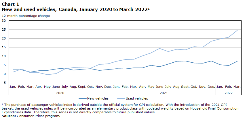
Data table for Chart 1
Chart 1
New and used vehicles, Canada, January 2020 to March 2022Note 1
Table summary
This table displays the results of Data table for Chart 1 New vehicles and Used vehicles, calculated using 12-month percentage change units of measure (appearing as column headers).
|
New vehicles |
Used vehicles |
| 12-month percentage change |
| 2020 |
|
| January |
2.27 |
1.03 |
| February |
2.24 |
2.78 |
| March |
1.03 |
0.73 |
| April |
1.88 |
0.68 |
| May |
1.98 |
-0.49 |
| June |
2.82 |
0.20 |
| July |
3.29 |
2.80 |
| August |
2.19 |
3.62 |
| September |
2.69 |
3.36 |
| October |
2.94 |
3.33 |
| November |
2.01 |
5.30 |
| December |
2.45 |
5.62 |
| 2021 |
|
| January |
2.87 |
7.11 |
| February |
2.79 |
8.13 |
| March |
3.49 |
8.24 |
| April |
3.39 |
10.20 |
| May |
4.94 |
11.73 |
| June |
4.10 |
14.44 |
| July |
5.52 |
12.61 |
| August |
7.13 |
13.82 |
| September |
7.22 |
13.57 |
| October |
6.13 |
15.28 |
| November |
6.03 |
14.98 |
| December |
7.21 |
18.32 |
| 2022 |
|
| January |
5.20 |
19.71 |
| February |
4.70 |
20.64 |
| March |
7.20 |
24.50 |
The introduction of used vehicle prices with the 2021 CPI basket will secure against future divergences in trend from new vehicle prices.
Comparison of used vehicle prices in Canada and the United States
While similar trends in the passenger vehicle market, where growth in used vehicle prices is currently outpacing growth in new vehicle prices, have been observed in both countries, Canadian consumers have not seen price increases of the magnitude of those observed in the United States.
There are key market differences between the two countries. Given the different sizes and scopes of automobile manufacturing in Canada and the United States, price movements may vary between the two countries for individual models. Not all used vehicles have shown the same price movements in the past year, with some classes of vehicle increasing in price significantly more than others. Sample composition, which is, in turn, influenced by what class of vehicles consumers are buying in Canada compared with the United States, may be contributing to the divergence in prices between the two countries. There is further potential for sample composition effects at the lowest level of detail because of differences in terms of available models in each country.
While both Statistics Canada and the Bureau of Labor Statistics (BLS) use a net household expenditures approach to calculating used vehicle weights, the weights are markedly different in the two countries. Passenger vehicles comprise 9.29% of the United States CPI basket of goods and services, compared with 6.21% in Canada. Of that weight, used vehicles make up 4.14% of the basket in the United States, compared with 1.84% in Canada’s 2020 CPI basket. These differences may also contribute to a different pre-pandemic seasonal pattern in Canada compared with the United States.
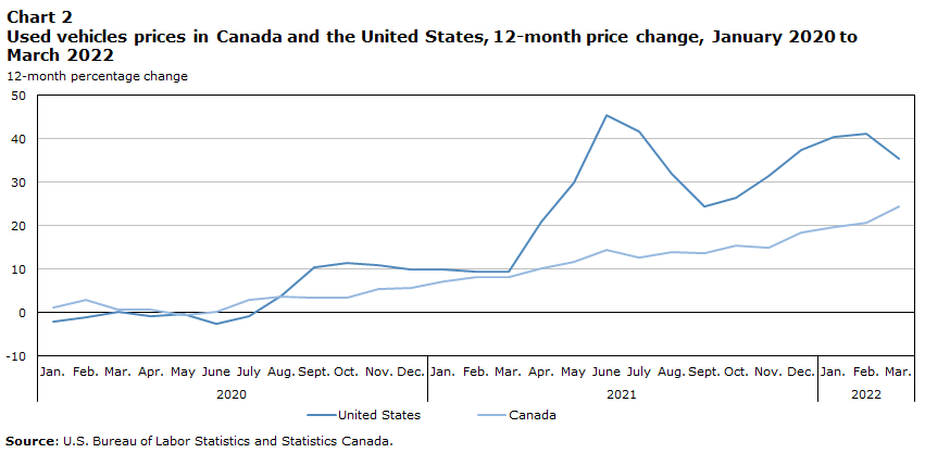
Data table for Chart 2
Chart 1
New and used vehicles, Canada, January 2020 to March 2022
Table summary
This table displays the results of Data table for Chart 2 United States and Canada, calculated using 12-month percentage change units of measure (appearing as column headers).
|
United States |
Canada |
| 12-month percentage change |
| 2020 |
|
| January |
-2.00 |
1.03 |
| February |
-1.20 |
2.78 |
| March |
0.10 |
0.73 |
| April |
-0.80 |
0.68 |
| May |
-0.30 |
-0.49 |
| June |
-2.70 |
0.20 |
| July |
-0.90 |
2.80 |
| August |
4.00 |
3.62 |
| September |
10.30 |
3.36 |
| October |
11.50 |
3.33 |
| November |
10.80 |
5.30 |
| December |
10.00 |
5.62 |
| 2021 |
|
| January |
10.00 |
7.11 |
| February |
9.40 |
8.13 |
| March |
9.40 |
8.24 |
| April |
21.00 |
10.20 |
| May |
29.80 |
11.73 |
| June |
45.30 |
14.44 |
| July |
41.60 |
12.61 |
| August |
31.90 |
13.82 |
| September |
24.40 |
13.57 |
| October |
26.40 |
15.28 |
| November |
31.40 |
14.98 |
| December |
37.30 |
18.32 |
| 2022 |
|
| January |
40.51 |
19.71 |
| February |
41.15 |
20.64 |
| March |
35.30 |
24.50 |
Recent market conditions are likely also at play. Between Canada and the United States, there have been significant differences in the scope and duration of public health measures introduced to limit the spread of COVID-19, as well as the economic supports offered. While periodic stimulus cheques were sent to Americans, the Canadian government provided more consistent, targeted supports to those who had lost employment as a result of the pandemic. Notably, the biggest spike in used vehicles prices in the United States occurred between April and June 2021, which coincided with the third stimulus payment, tax refund seasonNote 12 and an end to public health measures in many jurisdictions. An equivalent movement was not observed in Canada, which remained under some form of lockdown in much of the country until July 2021. Lockdown policies themselves may have also played a role in shifting demand: as prices for used vehicles surged in the United States during the spring of 2021, Canadians, who were re-entering lockdown measures in several provinces, reduced their mobility rates to a greater extent than their American counterparts.Note 13
There are also two differences in the methodological approaches used by the two countries:
- Statistics Canada uses a hedonic model, while the United States BLSNote 14 uses option cost adjustment based on information from car dealerships for quality adjustment;
- Different price data sources are used, with Statistics Canada using transaction data from point of sale and the BLS using assessment valuation data from an industry guide.
Impact on headline CPI
An analytical series was calculated to assess the impact of introducing used vehicle prices on the headline CPI. Given the weight of used vehicles (1.84%) in the 2020 CPI basket, if used vehicle prices had been introduced with the June 2021 CPI, coinciding with the last basket update, the headline CPI for March 2022 is estimated to have been 0.2 percentage points higher, compared with the published CPI (+6.7%).
2021 CPI basket
The introduction of the 2021 CPI basket will mark the implementation of the above enhancements to the calculation of the purchase of passenger vehicles index and the introduction of used vehicle prices to the CPI. At this time, the used vehicles index will be added to the CPI classification as a published aggregate:
- Transportation
- Private transportation
- Purchase, leasing and rental of passenger vehicles
- Purchase and leasing of passenger vehicles
- Purchase of passenger vehicles
- Purchase of automobiles (2013=100)Note 15
- Purchase of trucks, vans and sport utility vehicles (2013=100)Note 15
- Purchase of new passenger vehicles (2022-04=100)Note 16
- Purchase of used passenger vehicles (2022-04=100)Note 16
Because the CPI is a non-revisable index, used vehicle prices are proposed to be introduced with the May 2022 monthly price change with no level adjustment for historical price changes. This approach is consistent with the way other products have been included in the CPI such as cellular services, electronic devices and cannabis. This approach follows international best practices as well as the Consumer Price Index Manual (Chapter 7) and recommendations by Statistics Canada’s Price Measurement Advisory Committee. Although this type of ‘catch-up’ adjustment would account more fully for the impact of the recent increases in Canadian used vehicle prices in the CPI, it would be problematic for indexation and escalation of contracts that took effect in the past.
In summary
As of the introduction of the 2021 CPI basket, a new approach for measuring price change in used vehicles is recommended to replace the previous method of measuring used vehicles price change by proxy.
Statistics Canada continues to work with price experts, national statistical organizations and other partners to ensure data and methods used in the calculation of the CPI are aligned with international standards and best practices. The agency is continuing to monitor prices for used vehicles and acquiring new data sources for the measurement of the purchase of passenger vehicles index ensures the ongoing accuracy and relevance of the CPI.
For additional information or to provide comments on the proposed enhancement, users may contact the Consumer Prices Division at statcan.cpddisseminationunit-dpcunitedediffusion.statcan@canada.ca.
References
Akay, E., Bolukbasi, O., & Bekar, E. (2018). Robust and resistant estimations of hedonic prices for second hand cars: an application to the Istanbul car market. International Journal of Economics and Financial Issues 8(1), 39-47.
Bode, B., & van Dalen, J. (2001, April 2-6). Quality-corrected price indexes of new passenger cars in the Netherlands, 1990-1999 [Presentation]. International Working Group on Price Indices, Canberra, Australia.
Cheng, J. (2015, May 20-22). Quality adjustment of second-hand motor vehicle – application of hedonic approach in Hong Kong’s consumer price index [Presentation]. Ottawa Group on Price Indices, Ottawa, Canada.
de Haan, J., & Hendriks, R. (2013, November 28-29). Online data, fixed effects and the construction of high-frequency price indexes [Presentation]. Economic Measurement Group Workshop, Sydney, Australia.
de Haan, J., & Krsinich, F. (2018). Time dummy hedonic and quality-adjusted unit value indexes: do they really differ?, Review of Income and Wealth 64(4), 757-770.
Krsinich, F. (2014). Quality adjustment in the New Zealand Consumers price index. In S. Forbes & A. Victorio,The New Zealand CPI at 100. History and Interpretation. Victoria University Press.
Larsen, M. (2011, March 25). Experimental use of hedonics for new cars in the Danish HICP [Presentation]. Ottawa Group on Price Indices, Ottawa, Canada.
Nielsen, M. (2018, May 7-9). Quality adjustment methods when calculating CPI [Presentation]. Meeting of the Group of Experts on Consumer Price Indices, Geneva, Switzerland.
Reis, H. & Silva, J. (2002). Hedonic price indexes for new passenger cars in Portugal (1997-2001). Economic Bulletin and Financial Stability Report Articles and Banco de Portugal Economic Studies, Bank of Portugal, Economics and Research Department.
Requena-Silvente, F., & Walker, J. (2006). Calculating hedonic price indices with unobserved product attributes: an application to the UK car market. Economica 73(291), 509-532.
Tomat, G. (2002). Durable goods, price indexes and quality change: an application to automobile prices in Italy, 1988-1998. European Central Bank Working Paper.
Varela-Irimia, X. (2014). Age effects, unobserved characteristics and hedonic price indexes: the Spanish car market in the 1990s. SERIEs: Journal of the Spanish Economic Association 5(4), 419-455.
