
Publications
Rural and Small Town Canada Analysis Bulletin
Self-contained labour areas: A proposed delineation and classification by degree of rurality
Data and definitions

Archived Content
Information identified as archived is provided for reference, research or recordkeeping purposes. It is not subject to the Government of Canada Web Standards and has not been altered or updated since it was archived. Please "contact us" to request a format other than those available.
Box 1
Definitions of geographies
Census subdivision
Census subdivisions (CSD) are the building blocks of this analysis. A CSD is a municipality (i.e. incorporated town, rural municipality, city, etc. determined by provincial legislation) or its equivalent such as Indian reserves, Indian settlements and unorganized territories. In the 2006 Census of Population, there were 5,418 CSDs. For a detailed description of a CSD, see Statistics Canada (2007). CSDs can vary tremendously in terms of population size – from a few residents to over 2 million residents in Toronto. Also, the geographic spread of a CSD can vary widely – from less than 1 square kilometre for a small rural town to large geographic expanses of so-called "unorganized" territories in northern parts of many provinces. CSDs are aggregated into types of areas, as explained below, according to Statistics Canada's Statistical Area Classification (Statistics Canada, 2007).
Larger urban centres versus rural and small town areas
Larger urban centres (LUCs) are composed of CSDs classified as part of census metropolitan areas (CMAs) and census agglomerations (CAs).
- In 2006, a CMA was defined as having an urban core of 50,000 or more with a population of 100,000 or more after one includes all neighbouring CSDs where 50% or more of the resident workforce commutes to the urban core of the CMA.
- In 2006, a CA was defined as having an urban core of 10,000 or more and included neighbouring CSDs where 50% or more of the resident workforce commutes to the urban core of the CA.
-
- Larger CAs are census agglomerations with 50,000 or more residents. These CAs have census tracts designated within the CA and are also known as "tracted CAs."
- Smaller CAs are census agglomerations with less than 50,000 residents. These CAs do not have census tracts designated within the CA and are also known as "non-tracted CAs."
Rural and small town (RST) areas are CSDs which are not part of a CMA or CA. RST areas are further classified into a Metropolitan Influenced Zone (MIZ), as follows:
- Strong Metropolitan Influenced Zone: CSDs in a RST area where 30% or more of the resident workforce commutes to any CMA or CA;
- Moderate Metropolitan Influenced Zone: CSDs in a RST area where 5% to 29% of the resident workforce commutes to any CMA or CA;
- Weak Metropolitan Influenced Zone: CSDs in a RST area where more than zero but less than 5% of the resident workforce commutes to any CMA or CA;
- No Metropolitan Influenced Zone: CSDs in a RST area where none of the workforce commutes to a CMA or CA (or the workforce is less than 40 workers); and
- RST T erritories : CSDs in the Yukon, Northwest Territories and Nunavut which are outside the CAs of Whitehorse and Yellowknife.
Census rural population
Census rural: This is the definition of rural used by Statistics Canada's Census of Population. This definition has changed over time (see Appendix A in du Plessis et al., 2002). Typically, it has referred to the population living outside settlements of 1,000 or more inhabitants. The current definition states that census rural is the population outside settlements with 1,000 or more population with a population density of 400 or more inhabitants per square kilometre (Statistics Canada, 2007).
End of text box 1
Box 2
Data: Place of work and commuting flows
All the data used in this analysis are from the 2006 Census of Population and are tabulated at the census subdivision level. The data are derived from the place of work and place of residence variables (journey-to-work), which are used to generate commuting flow tables from the place of residence to the place of work. Details are provided below.
Place of work data
"Place of work data" refers to information derived from responses to the place of work question on the Census of Population. In 2006, the question on place of work appeared only on the long census questionnaire, which was sent to one in five households (20% sample of the population). The question appeared as follows: "At what address did this person usually work most of the time?" The choice of responses are: (1) Worked at home (including farms); (2) Worked outside Canada; (3) No fixed workplace address; and (4) Worked at the address specified below.
Commuting flow data (i.e. the data used in this analysis) are derived only when the response to this question is (4) and a specific address is provided. It should be noted that in 2006, for CMAs and CAs, the "specified" work address was coded at the level of the block-face, dissemination block or dissemination area representative point. The workplace location of persons working in RST areas was coded to census subdivision (CSD) representative points (Statistics Canada, 2007).
Commuting flow tables
The commuting flow tables measure how many people travel between the various areas of Canada. Each flow contains an origin area, a destination area and a count to represent the number of people traveling from the origin to the destination. Individuals with any particular "A" to "B" commuting flow can then be further described by other census variables (such as age, sex, occupation, level of educational attainment, etc.).
Out-of-scope census subdivisions
Not all CSDs could be grouped into self-contained labour market areas.
Among the 5,418 CSDs in Canada in 2006, there were 1,256 CSDs for which there were no commuting flows. These CSDs are generally small and thus there was no commuting or the commuting data were suppressed for reasons of data quality or to maintain confidentiality. These "out-of-scope" CSDs included 128,164 inhabitants (0.4% of Canada's population) (Appendix Table A1).
Another 336 census subdivisions showed no in-commuting and no out-commuting but there was commuting within the CSD (i.e. some individuals responded to "(4) Worked at the address specified below" and provided an address within the given CSD). In terms of commuting flows, these CSDs were 100% self-contained. These CSDs comprise two types of CSDs:
- CSDs that are remote and therefore daily commuting between any of these CSDs and any neighbouring CSD is not feasible. There are 9 CSDs with a population over 2,500 that are 100% self-contained (Appendix Table A1) and it is likely that these CSDs could be described as remote:
- Kitimat (British Columbia) (2006 population = 8,987);
- Revelstoke (British Columbia) (2006 population = 7,230);
- Iqaluit (Nunavut) (2006 population = 6,184);
- Mackenzie (British Columbia) (2006 population = 4,539);
- Grande Cache (Alberta) (2006 population = 3,783);
- Inuvik (Northwest Territories) (2006 population = 3,484);
- Lebel-sur-Quévillon (Quebec) (2006 population = 2,729);
- Fermont (Quebec) (2006 population = 2,633); and
- St. Theresa Point (Manitoba) (2006 population = 2,632).
- In addition, there were smaller CSDs for which commuting is possible. Note that commuting flows were suppressed for CSDs with less than 20 workers commuting to any given CSD or less than 20 workers commuting from any given CSD. Examples of smaller CSDs are the Saskatchewan towns of:
- Sintaluta (2006 population = 98);
- Chamberlain (2006 population = 108); and
- Alsask (2006 population = 129).
Each of these towns is located on a major highway with neighbouring towns within easy driving distance so commuting interactions would be expected. However, it is not surprising that there would be less than 20 commuters to or from any given neighbouring town.
Thus, due to remoteness or due to a small number of commuters, there are 336 CSDs that are in-scope but comprise their own 100% self-contained labour area.
The remaining 3,826 CSDs were grouped into 349 self-contained labour market areas (Appendix Table A1). These clusters represent the highest level of self-containment achievable for each grouping according to the model (Box 3) which required a minimum self-containment for each cluster along a sliding scale from 75% to 90%. Very few clusters were completely defined by their minimum value, with an average result of 96% self-containment for the 349 clusters under discussion.
Interestingly, a few of the 3,826 CSDs that were assigned to one of the 349 clusters had no workers residing in the CSD but had some workers commuting into the CSD – which would be the case if a plant or mine site was in a municipality adjacent to the incorporated town-site where the workers resided.
It is important to emphasize that possible merging of the 336 CSDs with no commuters with larger SLA clusters cannot be based on commuting flow criteria, but has to be based on other criteria. In the present analysis, we did not incorporate any additional criteria (e.g. proximity) to assign these CSDs to a SLA. This is because the result of self-containment or lack of commuting connectivity is an interesting finding on its own. However, in the discussion of the results, we do not focus our attention on these 336 CSDs that appear to be 100% self-contained labour areas. They appear to be a group of their own that deserves further attention (or possible re-aggregation based on additional criteria). We present some data on these CSDs in Appendix Tables A1, A3 and A4.
End of text box 1
Box 3
Methodology
The delineation of self-contained labour areas (SLAs) was based on a clustering procedure using data on the reciprocal flows of commuters. The method is derived from the algorithm developed by Bond and Coombes (2007) and the implementation of the algorithm was done in the SAS programming language. The main features of the method are outlined below while the details are presented in a forthcoming technical paper (Munro et al., forthcoming).
Clustering algorithm: focus on reciprocal importance of commuting flows
The algorithm used in this analysis has specific features that make it useful for the purpose of discovering rural labour areas. We used an algorithm based on the principle of "reciprocal importance" to indicate the strength of the linkage between any two census subdivisions (CSDs). The algorithm at the core of the clustering procedure shows a stronger linkage between two areas if the flows between any two areas are proportionally important to both areas. Specifically, our measure of reciprocal importance (RI) is:
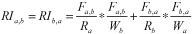
where F is the flow of workers (number) who commute from one CSD to another (a to b, or b to a); R is the number of workers who reside in the CSD (a or b), regardless of where they work; W is the number of workers who work in the CSD, regardless of where they live; and a and b are the subscripts for any pair of CSDs.
Reciprocal importance describes our desire to indicate that a given commuting flow from a to b is proportionally significant to both "A" area and "B" area. As an illustration of this concept, take a situation where 100 workers are leaving area A to go to area B. If area A is a large city with hundreds of thousands of resident workers, then the departure of those 100 workers is not particularly important to area A. If however area A is a very small town with only 200 resident workers overall, then this flow is very important to area A. Thus, a given flow between two smaller towns would generate a higher reciprocal importance (RI) than with the same flow between a smaller and a larger place. Using this example, the concept of reciprocal importance means that the algorithm will tend to group smaller areas together in order to produce larger increases in self-containment (defined below). This means that this algorithm is more likely than the other possible algorithms to discover self-contained labour areas among relatively smaller settlements.
Other key features of the procedure are that:
- All things being equal, this procedure tends to group smaller areas together first. This occurs because a relatively small flow can represent a significant proportion of commuters for a smaller area, and thus will produce a stronger linkage (i.e. a larger RI) than it would if it occured in a larger area. Additionally, larger areas are more likely to have a greater number of areas contributing or receiving its commuters, which leads to a relative reduction in the importance of any given connection.
- In comparison to clustering methods that take pre-defined urban areas as set starting points for each cluster, this procedure minimizes the urban bias by repeatedly selecting for the CSD or CSD group with the lowest degree of self-containment, regardless of classification.
- This procedure requires a higher level of self-containment for very small areas, which prevents small areas from reaching completion while significant flows remain, even if those flows are to or from a larger urban area.
Self-containment
Self-containment is a measure of the degree to which the workers living in "A" are also working in "A". Thus, by clustering areas with a high reciprocal importance of commuting flows and a low level of self-containment, we can create new areas with increasingly higher degrees of self-containment. Once a certain threshold for self-containment has been reached, this would then be considered a self-contained labour market because most residents with jobs are working in the given labour area and most individuals living in the given labour area are also working in the given labour market area.
It is important to note that self-containment is defined by two components. First, the self-containment of workers: the percent of workers in the area that also live in that area; and second, the self-containment of residents: the percent of residents in the area that also work in that area. Throughout this bulletin, whenever the term self-containment is used it refers to the combination of both of these components.
In order to define a threshold for self-containment we used a sliding scale that requires a higher degree of self-containment if the area (CSD or grouping of CSDs) has a small(er) resident labour force. Accordingly, for CSDs with under 1,000 resident workers, we set the minimum self-containment level to be 90%. For larger CSDs (with over 25,000 resident workers), our self-containment level was lower (at 75%). Hence, regardless of the size of the area, the minimum self containment of any SLA is 75%. There are two reasons for using a sliding scale to set the self-containment threshold. First, to ensure that smaller labour areas are not formed by excluding large numeric connections, we have used a higher threshold of self-containment where a smaller labour area is delineated as a self-contained labour area; and second, in order to avoid agglomerating all urban areas in Canada into one enormous labour area, larger areas need to have a lower threshold of self-containment to be designated as a self-contained labour area.
End of text box 1
- Date modified: