
Reports on Special Business Projects
Enhancing data for rural Canada: Small area estimation of remote work opportunities
Text begins
Executive summary
Rural Canada is characterized by dispersed and diverse communities with low population density. Estimates generated by surveys are usually produced by metropolitan area, but in rural areas, samples are typically too small to afford geographically granular estimates. Consequently, social and economic statistics at a small geographic scale are typically lacking. This causes the diversity of rural conditions to be masked by one aggregate average for “rural.”
This analysis illustrates how paucity of rural statistics can be mitigated by using estimation approaches with current survey samples combined with other existing data holdings. This analysis applies small area estimation (SAE) methods to selected indicators of remote work generated by the quarterly Canadian Survey on Business Conditions. The geographic concept used to obtain granular estimates for rural areas is that of the self-contained labour area (SLA), which represents a rural labour market or rural functional area.
- SAE methods are statistical techniques used to estimate population characteristics for small domains, such as neighbourhoods or rural areas, where sample sizes are typically too small to generate reliable estimates. In such a situation, SAE calibrates appropriate statistical models that link survey data to auxiliary data available for the entire population and produces parameter estimators that cover both the sampled and non-sampled domains of interest.
- In this analysis, the variable of interest is the proportion of businesses where remote work is possible for a given domain, which is a combination of geographic area and general industrial sector. The survey sample data are from the Canadian Survey on Business Conditions, for all four quarters of 2022. Auxiliary data sources include the Generic Survey Universe File created from Statistics Canada’s Business Register System and the 2021 Census of Population.
- For each quarter of 2022, survey data cover around 570 domains, compared with 1,263 domains available from final SAE estimates, which are significant supplements of the survey data. The domains cover almost all geographical areas in Canada, including census metropolitan areas and census agglomerations, representing urban areas and, for rural areas, SLAs, which are groups of census subdivisions connected by reciprocally important commuting flows between themselves.
- With fairly full coverage of Canadian geographical areas and a breakdown of general industrial sectors of service providers and goods producers, the study has key analytical insights into the behaviour of businesses in terms of remote work arrangements, with a quarterly trend in 2022.
- Rural areas are as diverse as urban areas in terms of businesses providing remote work opportunities. Not surprisingly, given the diversity of socioeconomic conditions and industry base of rural regions, their labour markets are driven by diverse conditions.
- As evidenced from the pooled results for all quarters and domains, businesses in rural and urban areas and in goods and services sectors behaved differently in making remote work arrangements. This informs the importance of distinguishing between rural and urban areas and the industrial sectors when analyzing the intention of businesses to offer remote work opportunities.
- Business preferences varied quarter over quarter in 2022 in arranging remote work for their employees. Their anticipation of work arrangements changed over time, depending on such factors as improvements by businesses of their technological and digital security conditions and the decreasing severity of the pandemic. Accordingly, the tendencies of businesses may change from time to time to respond to the relevant situation.
- As evaluated by the standard deviation, rural areas had less variability in final estimates of proportions than urban areas, across all quarters in 2022. Hence, remote work opportunities in rural labour markets tended to be relatively more stable than in urban areas.
- For rural areas, as measured by the median value, proportions of businesses offering remote work opportunities in the services sector were higher than their goods sector counterparts in three quarters of 2022 and edged down quarter over quarter.
- In a percentile analysis of rural domains, the final estimates of the top and bottom 5% grouped by quarter were identified, where the top 5% were defined as the most-possible domains and the bottom 5% the least-possible domains. It was found that some most- and least-possible domains in rural areas were not consistent over quarters. Instead, their quarterly estimates fluctuated between the upper and lower ranges, and the majority (70%) of businesses in these domains fell in the services sector.
1. Introduction
In a sample survey, sample sizes are usually not sufficient to generate direct estimates of adequate precision for small areas or domains. This is a challenge for rural areas in particular, where populations are small and dispersed across space. In such a situation, small area estimation (SAE) calibrates appropriate statistical models that link survey data to auxiliary data available for the entire population. In other words, SAE “borrows strength” through auxiliary information to produce reliable indirect estimates.
This experimental study applies an area-level SAE model to estimate the proportion of businesses where remote work was possible at the domain level, for each quarter of 2022 of the Canadian Survey on Business Conditions (CSBC). In the study, a domain is a combination of geographic area and general industrial sector. The disaggregation by geographic area used in this analysis allows the generation of more granular data for rural regions by using a novel geographic concept, the self-contained labour area (SLA) (OECD, 2020). Geographic areas (census subdivisions [CSDs]) are classified as urban areas when they are part of a census metropolitan area (CMA) or census agglomeration (CA), while they are defined as rural when they jointly form an SLA.
The motivation for this study is twofold. First, rural regions present a diversity of economic and social conditions; nevertheless, it is widely recognized that timely and geographically granular information on these regions is often lacking. Second, since the onset of the COVID-19 pandemic in March 2020, Canadian businesses have taken actions to make remote work arrangements for their employees. In this regard, businesses located in small rural areas and urban areas may behave differently, and rural businesses specializing in the goods sector and the services sector are also hypothesized to act in a different way.
Remote work, one element of this rural–urban diversity, has received considerable policy attention since the onset of the pandemic. As pandemic conditions changed, businesses adjusted their policies to offer remote work opportunities, and such a change may vary from area to area and from quarter to quarter. This motivates the study in terms of the proportion of businesses where remote work was possible, focusing on small rural areas and on a quarterly basis.
The remainder of this paper is structured as follows. The domain and the business indicator of interest originating from the CSBC are defined and discussed in Section 2 and Section 3. Section 4 introduces the direct point and variance estimators. Section 5 describes an area-level model for proportion, variance smoothing, the auxiliary data sources and the R package used to calibrate the SAE model. Model results are also discussed in this section. Model performance evaluation and analytical findings of final estimates are reviewed in Section 6 and Section 7. Section 8 concludes the paper with future directions of study.
2. Domain of interest
As noted by Rao and Molina (2015), domains may be defined by geographic areas or sociodemographic groups or other subpopulations. A domain is regarded as large (or major) if the domain-specific sample is large enough to yield direct estimates of adequate precision. A domain is regarded as small if the domain-specific sample is not large enough to support direct estimates of adequate precision.
The current study defines a domain as a combination of geographical area and general industrial sector. Geographical area types include CMAs, CAs and rural SLAs, which are all delineated from granular CSDs, based on the 2016 Standard Geographical Classification.Note
A CMA has a total population of at least 100,000, of which 50% or more must live in the core, and a CA has a core population of at least 10,000 but has no other total population requirement (Statistics Canada, 2022). Municipalities (CSDs) belong to a CMA or CA if they are highly integrated with the core, as measured by commuting flows. SLAs make up the geographic areas that do not belong to CMAs or CAs. According to Munro et al. (2011), SLAs are created by grouping CSDs that represent reciprocally important commuting flows between themselves. The clustering algorithm focuses on reciprocal importance of commuting flows obtained from the 2016 Census of Population. The algorithm at the core of the clustering procedure shows a stronger linkage between two areas if the flows between them are proportionally important to both areas. It has specific features that make it useful for the purpose of discovering rural labour areas. The procedure delineates SLAs consisting of two or more CSDs where the majority of the workers live and work in the same area, hence fulfilling the self-containment requirement. As per the Organisation for Economic Co-operation and Development (OECD, 2020), self-containment has two aspects: (1) self-containment of workers (percentage of area jobs that are filled by area residents) and (2) self-containment of residents (percentage of area residents who have jobs in the area). The minimum threshold for self-containment is 75%.
CMAs and CAs are essentially urban areas, and SLAs are rural areas. When an area overlaps two provinces, it is considered as two distinct areas. Overall, there are 36 CMAs, 120 CAs and 504 SLAs that are delineated from 5,162 CSDs as building blocks from the 2016 Standard Geographical Classification.
In terms of industrial classification, businesses registered in each CSD are classified into two general industrial sectors based on their North American Industry Classification System (NAICS) codes.Note These are goods producers (NAICS 11 to 33) and service providers (NAICS 41 to 91), each with some out-of-scope subsectors aligned with the corresponding survey data. At the upper level, the combination of CMA, CA or SLA and the general industrial sectors forms the domain of interest in this study. The total number of domains is determined by the available data from the auxiliary data file that is used as the business population. This is further discussed in Section 5.3. Altogether, 1,263 domains are established from 640 geographical areas.
3. Target business indicator
The purpose of the CSBC is to collect information on business expectations and conditions in Canada, as well as emerging issues. The target population for this survey is all active establishments on the Business Register (BR) with an address in Canada and with employees. The following NAICS subsectors and sectors are excluded from the target population. Accordingly, the definition of general industrial sectors also excludes these categories from this study:
- 22: utilities
- 523990: all other financial investment activities
- 55: management of companies and enterprises
- 611: educational services
- 6214: out-patient care centres
- 6215: medical and diagnostic laboratories
- 6219: other ambulatory health care services
- 622: hospitals
- 814: private households
- 91: public administration.
This study focuses on the business indicator of working arrangement from the quarterly CSBC. Specifically, for a given domain, what is the proportion of businesses where remote work is possible? This target question is not directly addressed in the 2022 CSBC. Instead, the survey asked questions in the following way (Statistics Canada, CSBC questionnaire):
Over the next three months, what percentage of the employees of this business or organization is anticipated to do each of the following?
Exclude staff that are primarily engaged in providing driving or delivery services or staff that primarily work at client premises.
Provide your best estimate rounded to the nearest percentage. If the percentages are unknown, leave the question blank.
- Work on-site exclusively
- Work on-site most hours
- Work the same amount of hours on-site and remotely
- Work remotely most hours
- Work remotely exclusively
Respondents could provide a percentage for each answer option. For any valid response, if the percentage points from A and B add up to 100%, this implies that it is not possible to work remotely in the sampled business. In such a case, a flag of “No” is assigned. Otherwise, an indicator of “Yes” will be coded. This procedure converts the five numeric variables into a binary variable, which leads to an estimate of the proportion of businesses where remote work is possible, for a given domain.
4. Direct estimate and variance
4.1 Direct point estimator
The direct point estimator for a given domain d is derived using recoded sample data and the survey sample weight. It is given by Equation (1) below:
where denotes the direct point estimator of the proportion of businesses where remote work is possible in domain d, W is the survey sample weight, i denotes the ith firm in domain d, and is the indicator that the ith firm is recoded Yes to the binary variable.
4.2 Variance estimator
Any estimates derived from samples are subject to sampling error, measured commonly by the sampling variance, which depends on many things, including the sampling method, the estimation method, the sample size and the variability of the estimated characteristic (Statistics Canada, 2021). The CSBC uses a stratified random sample of business establishments classified by geography, industry sector and size (for detailed information, see Statistics Canada, CSBC Integrated Metadatabase). It applies a two-phase stratified simple random sampling design, with the second phase accounting for the non-response from the survey. In the second phase, reweighting is performed on the responding units so that their final weights still represent the whole target population. After the reweighting, a calibration process is performed so that the weighted totals per calibration group equal the population totals. Because the point estimator of the proportion as shown in Equation (1) is a nonlinear estimator, and calibration is used, the Taylor linearization approachNote is adopted to estimate sampling variance. The variance estimation is performed using the Generalized Estimation System (Statistics Canada, 2019).
The variance estimator is a function of the sample size. As shown in Chart 1 using the first quarter of 2022, for a given domain, the larger the sample size, the smaller the estimated sample variance, and hence the more precise the point estimator would be.

Data table for Chart 1
The data is available in csv format.
5. Small area estimation
In the context of this study, SAE refers to the techniques that are applied to produce model-based estimators. The essence of SAE is the calibration of appropriate statistical models linking survey data with auxiliary data available at the small domain level. According to Rao and Molina (2015), the models are classified into two broad categories: (1) area-level models that relate the small area summary statistics to area-level covariates from auxiliary data sources and (2) unit-level models that relate the unit values of a study variable to unit-specific auxiliary variables. Different functional forms can be specified, depending on whether the type of response variable is continuous or discrete in nature. In the current study, the variable of interest is the proportion of businesses in each domain where remote work is possible, compared with the opposite scenario, where remote work is not possible. Because a binomial distribution applies, a logistic regression model is used.
5.1 Area-level model for proportion
The area-level model for a proportion is an application of the classic Fay–Herriot model (Fay and Herriot, 1979), with the dependent variable defined as the additive log ratio transformation of the direct estimators. It follows the estimation framework set up by Esteban et al. (2020), which can be specified in two stages. In the first stage, the sampling model is specified:
where is the population proportion of businesses in domain d where a remote work arrangement is possible. It depends on unknown regression parameters and auxiliary variables. represents sampling errors that are assumed to be normally distributed with zero mean and known variance of .
In the second stage, the linking model is defined:
where is a vector of auxiliary variables measurable for each domain d, is the vector of regression coefficients to be estimated, and is the domain-specific random effect with zero mean and variance .
In practice, the synthetic estimate is obtained by rolling up the estimated coefficients over the inverse of the additive log ratio transformation, such that:
The composite estimate is then calculated from the linking mechanism that combines the direct estimator and the synthetic estimator:
where denotes the shrinking factor that links domain-specific direct estimate variance to estimated random effect variance ( ) across all domains. That is,
where is estimated using the algorithm of restricted maximum likelihood (Rao and Molina, 2015) to proxy , and is the sample variance estimator. For a domain where no sample is drawn, reduces to zero and the composite estimate becomes the synthetic estimate .
5.2 Variance smoothing
At the domain level, sample variance can be unstable, especially for domains with small sample sizes. It is recommended, therefore, to smooth the variances in some way (Bocci et al., 2022). The steps given below show how variance smoothing is applied in this study, following methods from You and Hidiroglou (2022).
Step 1: Use a generalized variance function (GVF) with the Rivest and Belmonte (2000) correction factor
Assume there are m domains, and specify the log-log model:
From the model, the naïve GVF-smoothed estimator of the sampling variance, , is derived as , for each domain d. Also, the estimated residual variance of the model is defined as , where the model residual for domain d is .
The smoothed variance corrected by accounting for the residual variance (proposed by Rivest and Belmonte [2000]), , is computed as .
Step 2: Use a GVF with the Hidiroglou et al. (2019) correction factor
In this alternative approach, the smoothed variance, , is derived as , where is the correction factor across all domains and is calculated as .
Step 3: Use the design effect (DEFF) method
In this alternative approach, there is no need to calibrate the log-log model. For each domain, the estimated design effect, , is given by:
Where is the direct point estimator from (1).
Further, the average of , denoted as , is aggregated as , and the average of , denoted as , is . The smoothed variance, , is then given by:
Step 4: Take the average of the results from the three approaches above
In this practical application, we use both the GVF and DEFF smoothed estimates, following You and Hidiroglou (2022), and the final smoothed variance estimate, , is derived as .
The final smoothed variances are plotted with the variances calculated using the Taylor linearization approach on Chart 2, where the X-axis is the index number of domains, and the final smoothed variances are sorted ascendingly. It is shown that the final smoothed variances became less volatile, compared with the original variances. The final smoothed variances will then be used as in the SAE model as one of the important inputs.

Data table for Chart 2
The data is available in csv format.
5.3 Auxiliary data
Based on careful exploratory analysis, variables from two sets of data are selected as auxiliary data in the SAE process. The first is the business population data known as the Generic Survey Universe File (GSUF). The data are accessible from the Linkable File Environment maintained in Statistics Canada’s Centre for Special Business Projects. For the current study, the vintage of 2021 V18 data is used. This covers over 1.4 million businesses with employees, with all levels of businesses, including enterprises, establishments, companies and locations. Of these, only in-scopeNote establishments (a little over 1 million records) are selected to build the auxiliary file to have a reasonable population of interest.
For each domain, firm age and average goods and services tax (GST) modelled sales revenue are averaged and weighted by number of employees. Also, average firm age squared is used to capture the nonlinearity pattern of the firm age effect on the decisions of businesses. Even after aggregation, the average GST sales are skewed and do not follow a normal distribution. The log sales are used as a solution. In addition, area type is created to distinguish whether a geographic area is a CMA, a CA or a rural SLA. As previously mentioned, CMA and CA jointly define urban areas, and rural SLA represents rural area. Finally, a flag of general industrial sector is generated to further split a geographic area, as in the goods or the services sector.
The second auxiliary data source is the 2021 Census. This was explored in an attempt to explain the behaviours of businesses from the demographic aspect. For each CMA, CA and rural SLA, key demographic variables from the 2021 Census are aggregated. These include the percentage of young people (ages 15 to 34) out of total working-age population (ages 15 to 64), the percentage of households living in apartments out of all households and average household employment income in thousands of dollars.Note
All these variables form the vector found in Equation (3).
5.4 R package
The SAE is processed using the R package “sae.prop” (Sholihin and Sumarni, 2022), which implements SAE using Fay–Herriot models with additive logistic transformation (ALR). Specifically, the function mseFH.ns.uprop() is employed. This features the parametric bootstrap mean squared error (MSE) of empirical best linear unbiased predictors based on a univariate Fay–Herriot model with ALR for non-sampled data.
For domains with direct estimates between 0 and 1, composite estimates are calculated following Equation (5). For domains that have an extreme direct estimate of 0 or 1,Note or for domains with no sample data, synthetic estimates are calculated following Equation (4). For the current study, 500 iterations of bootstrapping are applied to estimate the MSE by domain, from which standard errors are derived.
5.5 Model results
The SAE model is calibrated for each individual quarter of 2022, with the same set of variables. The model result for the first quarter is reported in Table 1.
| Variables | Coefficient | Standard Error | t value | p value |
|---|---|---|---|---|
| Intercept | 5.1091Note ** | 2.4293 | 2.1031 | 0.0355 |
| General sector (services) | 0.2788Note * | 0.1451 | 1.9218 | 0.0546 |
| Average firm age | -0.3356Note * | 0.1825 | -1.8389 | 0.0659 |
| Average firm age squared | 0.0082Note * | 0.0044 | 1.8761 | 0.0606 |
| Average GST Sale in logarithm | -0.1723Note ** | 0.0825 | -2.0895 | 0.0367 |
| Percent of young persons (ages 15 to 34) out of total working age population (ages 15 to 64) | -3.8501Note ** | 1.5335 | -2.5107 | 0.0120 |
| Percent of number of households living in apartments out of all households | 1.7827Note ** | 0.8270 | 2.1557 | 0.0311 |
| Average household employment income in thousand dollars | 0.0112Note ** | 0.0046 | 2.4489 | 0.0143 |
| Area type (CMA) | 0.4695Note ** | 0.2341 | 2.0051 | 0.0450 |
| Area type (SLA) | 0.2053 | 0.1966 | 1.0441 | 0.2964 |
|
||||
From the above model, on one hand, service providers have an e0.2788 or 1.32 times the odds of goods producers of offering remote work opportunities. In other words, in the first quarter of 2022, businesses in the services sector had a 32% greater chance of arranging remote work, compared with those in the goods sector, when holding other variables constant. This result is statistically significant at a 10% level of significance informed by the p value. Activities in the services sector, such as data processing and banking, have a high potential for remote work, and employers are more likely to make such arrangements. On the other hand, the goods sector, such as manufacturing and crop production, usually requires physical presence and is therefore less likely to work remotely.
Along the same line of reasoning, at a 5% level of significance, businesses located in a CMA would be 60% (e0.4695-1) more likely to make remote work arrangements than the reference category of businesses in a CA. Businesses in rural areas (SLAs) have a probability of offering remote work arrangements that is significantly different from CAs.
Firm age aggregated at the domain level is found to be negatively associated with the log odds of the outcome (i.e., remote work is possible), but this relationship is not linear. The log odds of the outcome increase at a decreasing rate as average firm age increases. Quantitatively, an increase of one year in the average firm age is associated with a decrease of 29% (1- e-0.3356) in its likelihood of offering remote work opportunities. This suggests that older firms are less prone to arrange remote work, compared with newer businesses. However, the effect of age on the log odds of the outcome turns out to be marginally positive as an average firm gets older and is more technologically prepared to make remote work arrangements.
Holding other factors constant, an increase of one unit of GST sales rescaled in logarithm is associated with a 16% (1- e-0.1723) decrease for the willingness of businesses to offer remote work opportunities. This finding is at a 5% level of significance. Domains with higher average GST sales are possibly occupied by businesses with a traditional corporate culture that emphasizes the importance of on-site work to promote collaboration and innovation. But without additional information on firm characteristics, it is not possible to justify this.
From the demographic perspective, a higher percentage of young people in the total working population is related to a lower likelihood of remote work opportunities offered by businesses. It is estimated that a 1% increase in the proportion of young people is associated with a decrease of 98% (1- e-3.8501) in the chance that businesses would offer remote work opportunities. In terms of structural type of dwelling, a 1% increase in the percentage of households living in apartments is correlated to approximately five times (e1.7827-1) greater probability of arranging remote work, when holding other variables constant. With regard to income, a $1,000 increase in average household employment income is associated with an increase of 1% (e0.0112-1) in the chance of remote work arrangements.
The interpretation illustrated above is for each individual variable, holding other variables constant. Actual estimators are the result of scoring coefficients of all variables (including intercept), compounded by the linking mechanism shown in Equation (5), where applicable. Also, the same set of variables is used to calibrate models for other quarters, where the levels of significance are not necessarily the same as the model for the first quarter.
6. Model performance evaluation and result finalization
In this study, SAE model performance evaluation is conducted from two perspectives. The first is to apply diagnostics to examine model prediction power and analyze residuals. The second refers to a benchmarking process in which SAE estimates are aggregated to the higher level (such as the provincial level), where direct estimates are more reliable. In such a case, direct estimates are used as benchmarking values with which aggregated SAE estimates are compared. A final wrap up is done to determine final estimates to be produced.
6.1 Small area estimation diagnostics
Results from the CSBC for the first quarter of 2022 are used to demonstrate model performance diagnostics. Of the 1,263 domains based on the business population file (GSUF 2021 V18), there are 570 with composite SAE estimates. Scatterplots of SAE estimates vs. direct estimates are presented in Chart 3, grouped by area type (Panel A) and general industrial sector (Panel B), where R squared measures the proportion of the variation in the direct estimate captured by the SAE model.

Data table for Chart 3
The data is available in csv format.
The colours of R squared in Figure 3 are associated with the different categories examined. Classified by either area type or general sector, the SAE model can capture a large proportion (≥ 95%) of the variation in the direct estimate. Model performance is better for CMA domains than for CA and SLA domains, thanks to large sample sizes. Also, the model has the same (and high) predictive power for the goods sector and services sector.
For a residual analysis, the model residual is calculated as , where is the predicted log odds. Standardized model residual is plotted with standardized predicted log odds (Chart 4). It is shown that the residuals are randomly scattered around zero with no noticeable patterns for the majority domains, evidenced by the small R squared (< 0.01). This suggests that there is no strong evidence of heteroscedasticity. The generalized linear model has a good fit to the data, and the SAE estimates are robust to the residuals’ moderate deviations from normality.

Data table for Chart 4
The data is available in csv format.
Furthermore, the average variance from the direct estimates is compared with the average MSE from SAE, by area type (Chart 5). For CMAs where large sample sizes are available, direct estimates and SAE tend to have similar (and low) variances, suggesting that both approaches are subject to smaller sampling errors. For CAs and SLAs, however, SAE clearly has lower average variance (MSE) than the direct estimates. This leads to the conclusion that the estimated proportions from SAE are more reliable than those from direct estimates, for smaller domains.

Data table for Chart 5
| Average.Variance | |||
|---|---|---|---|
| CMA | CA | SLA | |
| percent | |||
| Direct Estimate | 1.001 | 2.978 | 3.125 |
| SAE | 0.981 | 1.602 | 1.791 |
| Source: CSBC (the first quarter of 2022), G-SUF 2021 V18, Census 2021, author’s calculations. | |||
6.2 Benchmarking: Aggregated small area estimation result compared with direct estimates
For the first quarter of 2022, the SAE estimates by domain are aggregated to the provincial, combined territorial and national levels, as well as the urban (CMA and CA) and rural (SLA) levels. To do this, for each granular domain, the SAE estimate is multiplied by the total number of in-scope businesses to derive the number of businesses where remote work is possible. The result is then aggregated to a higher level and divided by the total number of in-scope businesses at that level to convert back to a proportion. This is then compared with the direct estimate at the same level, where the sample size is large enough to produce a reliable estimate (Table 2).
| Aggregated SAE | Direct estimate | |||||
|---|---|---|---|---|---|---|
| Average | 95% Confidence intervalTable 2 Note 1 | Average | 95% Confidence intervalTable 2 Note 1 | |||
| percent | from | to | percent | from | to | |
| Canada | 36.7 | 32.5 | 39.5 | 36.8 | 35.0 | 38.7 |
| Newfoundland and Labrador | 30.9 | 26.8 | 33.4 | 28.1 | 24.7 | 31.6 |
| Prince Edward Island | 27.9 | 18.2 | 34.0 | 27.8 | 24.2 | 31.5 |
| Nova Scotia | 30.2 | 21.3 | 36.6 | 31.9 | 28.3 | 35.2 |
| New Brunswick | 26.7 | 21.0 | 31.4 | 25.6 | 22.6 | 29.1 |
| Quebec | 35.5 | 28.8 | 38.7 | 34.1 | 30.7 | 37.3 |
| Ontario | 38.8 | 31.2 | 42.2 | 39.5 | 35.7 | 43.7 |
| Manitoba | 28.7 | 20.0 | 32.1 | 28.9 | 25.2 | 32.5 |
| Saskatchewan | 29.4 | 24.6 | 33.2 | 27.8 | 24.5 | 31.1 |
| Alberta | 37.6 | 29.8 | 42.4 | 38.9 | 34.7 | 43.0 |
| British Columbia | 38.6 | 27.4 | 44.8 | 38.6 | 34.6 | 42.5 |
| Territories | 40.0 | 35.4 | 44.5 | 40.3 | 34.8 | 45.5 |
| Rural | 28.1 | 26.4 | 30.2 | 26.0 | 22.7 | 29.5 |
| Urban | 38.6 | 34.0 | 41.1 | 39.1 | 37.1 | 41.1 |
|
||||||
On one hand, the aggregated SAE estimates at the Canada level are comparable to the benchmark value of the direct estimates. A similar relationship is observed for urban areas. This is expected because, when sample sizes are large enough, the direct estimate is reliable and aggregated SAE essentially reproduces the direct estimate. On the other hand, SAE is slightly overestimated for rural areas, as well as for the Atlantic provinces (except Nova Scotia), Quebec and Saskatchewan. SAE is marginally underestimated for Nova Scotia, Ontario and Alberta. Additionally, SAE for Manitoba, British Columbia and the three territories combined (Nunavut, the Northwest Territories and Yukon) are comparable to the direct estimators. Further adjustments are foregone because the gaps between SAEs and direct estimators are modest and even close for larger domains (such as Canada and urban).
6.3 Final estimate
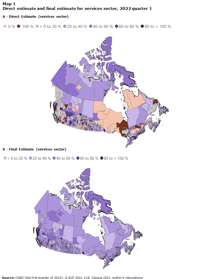
The final estimates are prepared by combining three sources of results. Because CMAs have a relatively larger sample size, their direct estimates and SAE estimates are very close (Figure 3.A), and the average variances from the direct estimates and SAE are also similar (Figure 5). Therefore, direct estimates are adopted for the CMA domains, if available. Otherwise, the SAE model estimates are used. For the SAE model estimates where the survey sample is available, the final estimate is the composite estimate that links the direct estimate with the model predicted value through the shrinking factor (Equation [6]); for the domains without sample or for those where the extreme direct estimate is 0 or 1, the final estimates are the synthetic estimates because they are derived from the model only.
The final estimates for the first quarter of 2022, classified by services and goods sector, are mapped (Map 1. B and Map 2. B) and compared with their direct estimate counterparts (Map 1. A and Map 2. A). Overall, there are 693 domains that do not have direct estimates (grey areas) or have extreme direct estimates. Of these, 609 (88%) are SLAs (rural areas). Visually, final estimates have fairly complete coverage of almost all geographical areas in Canada, thanks to the SAE approach using auxiliary data to supplement the CSBC.
Data table for Map 1
The data is available in csv format: Map 1-A Direct Estimate | Map 1-B Final Estimate.
Source: CSBC (the first quarter of 2022), G-SUF 2021 V18, Census 2021, author's calculations.

Data table for Map 2
The data is available in csv format: Map 2-A Direct Estimate | Map 2-B Final Estimate.
Source: CSBC (the first quarter of 2022), G-SUF 2021 V18, Census 2021, author's calculations.
7. Analytical findings
The analysis of the final estimates focuses on their distribution and variance by groups and provides a closer look into the industry composition in rural areas. Main analytical findings are discussed below.
- Businesses in rural and urban areas, and in the goods and services sectors, were substantially diversified in making remote work arrangements
For the final estimates with all four quarters of 2022 pooled, statistical testsNote are performed to detect whether the estimated proportions between rural and urban areas, and between goods producer and service providers, are distributed differently. In both cases, test results lead to rejecting the null hypothesis of the same target variable distribution between the two groups. Chart 6.A and B shows the distribution grouped by the two categorical variables. This informs the importance of distinguishing rural and urban areas and the industrial sectors when analyzing the intention of the businesses to offer remote work opportunities. Specifically, Chart 6.A shows that there is substantial diversity of remote work opportunities within rural areas. Three-quarters of the domains (951 out of 1,263) are rural, with a mean estimate of 0.274 and standard deviation of 0.144 from all quarters of 2022. Such a finding only becomes available using the SAE approach.

Data table for Chart 6
The data is available in csv format.
- The preferences of businesses varied quarter over quarter in arranging remote work for their employees
For the same pooled data, a statistical testNote is conducted to find whether the estimated proportions across the four quarters of the CSBC in 2022 distribute differently. In such a case, the null hypothesis of the same distribution across the four quarters is also rejected. Chart 7 below shows the distribution for each individual quarter. Since the original survey questions relate to businesses’ anticipation of work arrangements over the next three months, it is expected that this outlook changes over time, depending on such factors as improvements by businesses of technological and digital security conditions and the decreasing severity of the pandemic. Accordingly, the tendencies of businesses may change sometimes to respond to the relevant situation.

Data table for Chart 7
The data is available in csv format.
- Remote work opportunities in rural labour markets tend to be relatively more stable than in urban areas
Evaluated by the standard deviation, the rural SLAs had less variability in final estimates of proportions than urban areas across all quarters in 2022 (Table 3). The business population file of GSUF includes approximately 176,000 establishments from rural areas, accounting for about 18% of all establishments that were in scope for this analysis. By contrast, the number of rural domains (951) geographically was considerably larger than its urban counterpart (312). In terms of the industry composition, as of 2021, the rural areas contained 813 industrial sectors (six-digit NAICS codes) that were in scope for this analysis, less than their urban counterparts (848). Less coverage of industries in rural areas implies less diversified behaviour by businesses and hence impacts the standard deviation of the final estimates. Lastly, the weighted mean of the number of employees in rural areas (63) was far less than in urban areas (251). Businesses in rural areas with a relatively small number of employees may be more flexible in working arrangements. Individual estimates of a rural business may be more clustered around the group mean, resulting in a lower standard deviation.
| Rural | Urban | |||||||
|---|---|---|---|---|---|---|---|---|
| Mean | Standard deviation | 95% Confidence interval | Mean | Standard deviation | 95% Confidence interval | |||
| percent | from | to | percent | from | to | |||
| Quarter 1, 2022 | 28.1 | 13.5 | 27.3 | 29.0 | 28.4 | 15.9 | 26.6 | 30.2 |
| Quarter 2, 2022 | 27.8 | 14.7 | 26.9 | 28.7 | 26.3 | 17.2 | 24.4 | 28.2 |
| Quarter 3, 2022 | 27.6 | 13.9 | 26.7 | 28.5 | 25.6 | 15.1 | 23.9 | 27.2 |
| Quarter 4, 2022 | 26.1 | 15.3 | 25.1 | 27.1 | 27.6 | 17.1 | 25.7 | 29.4 |
| Source: CSBC (all quarters, 2022), G-SUF 2021 V18, Census 2021, author’s calculations. | ||||||||
- Rural businesses in the services sector were more likely to offer remote work opportunities than those in the goods sector, but with a quarterly downward trend
In rural areas, as measured by the median value of the estimated proportion, businesses in the services sector were more likely to arrange remote work, compared with the goods sector. The most noticeable gap between the two sectors was observed in the first quarter of 2022. However, as business conditions improved over the course of the pandemic, this difference decreased moderately over quarters (Table 4). The third quarter was an exception, which appeared to be an overreaction from the services sector to the easing of pandemic restrictions, in such a way that businesses were (slightly) less likely to offer remote work than the goods sector.
Overall, service providers edged down in offering remote work opportunities, from the first to the fourth quarters of 2022. This aligned with the fact that more businesses encouraged employees to return to the workplace as pandemic restrictions eased. Goods producers had a mixed response to this situation, although the fourth quarter showed the lowest percentage point of the willingness of businesses to allow remote work.
| Goods | Services | |||||||
|---|---|---|---|---|---|---|---|---|
| Median | Mean | 95% Confidence interval | Median | Mean | 95% Confidence interval | |||
| percent | from | to | percent | from | to | |||
| Quarter 1, 2022 | 23.4 | 25.2 | 24.1 | 26.2 | 29.6 | 31.1 | 29.8 | 32.4 |
| Quarter 2, 2022 | 23.6 | 26.7 | 25.4 | 27.9 | 25.7 | 28.9 | 27.5 | 30.3 |
| Quarter 3, 2022 | 25.8 | 28.0 | 26.8 | 29.1 | 24.4 | 27.2 | 25.9 | 28.6 |
| Quarter 4, 2022 | 22.7 | 24.8 | 23.6 | 26.0 | 23.6 | 27.4 | 25.9 | 28.9 |
| Source: CSBC (all quarters, 2022), G-SUF 2021 V18, Census 2021, author’s calculations. | ||||||||
- The most- and least-possible domains in rural areas were not consistent over quarters
In a percentile analysis of rural domains, the final estimates of the top and bottom 5% grouped by quarter were identified, where the top 5% are defined as the most-possible domains and the bottom 5% the least-possible domains where remote work arrangements were offered. All rural domains that had final estimates greater than or equal to the top 5% value, and less than or equal to the bottom 5% value, were then sorted. Of the overall 951 rural domains, there were 275, or nearly 30%, that fell in this range, either in one quarter or in multiple quarters. Of these, 24 were found in at least three quarters (Table 5).
| Domain | Final estimate of 2022 | |||
|---|---|---|---|---|
| Quarter 1 | Quarter 2 | Quarter 3 | Quarter 4 | |
| percent | ||||
| 10_6717_Services | Note ...: not applicable | 5.6 | 7.9 | 2.5 |
| 13_6532_Goods | 1.9 | 4.4 | 2.6 | 5.9 |
| 24_4591_Goods | 57.7 | 74.9 | 61.0 | 69.5 |
| 24_6025_Services | 5.8 | Note ...: not applicable | 6.2 | 3.5 |
| 24_6238_Services | 82.3 | 67.8 | Note ...: not applicable | 58.8 |
| 24_6252_Services | Note ...: not applicable | 3.8 | 79.1 | 3.9 |
| 24_6588_Goods | Note ...: not applicable | 66.1 | 61.3 | 3.2 |
| 24_6734_Services | 58.3 | Note ...: not applicable | 64.8 | 4.6 |
| 24_6830_Goods | Note ...: not applicable | 4.5 | 5.3 | 1.7 |
| 35_1000031_Goods | 62.9 | 76.9 | 59.0 | 81.2 |
| 35_6804_Services | 8.3 | 83.7 | 4.0 | 58.9 |
| 46_6778_Goods | 7.4 | Note ...: not applicable | 3.0 | 1.8 |
| 47_1000038_Goods | 58.0 | 69.6 | 57.1 | 77.2 |
| 47_4618_Goods | 59.0 | 73.2 | 58.3 | 80.4 |
| 47_5183_Services | Note ...: not applicable | 76.3 | 58.8 | 87.4 |
| 47_5907_Services | 5.9 | 2.3 | Note ...: not applicable | 1.4 |
| 47_6343_Goods | 64.2 | 74.4 | 56.6 | 75.3 |
| 48_1000059_Goods | Note ...: not applicable | 71.0 | 59.4 | 85.2 |
| 48_6337_Services | 59.0 | 69.8 | Note ...: not applicable | 4.0 |
| 48_6763_Goods | Note ...: not applicable | 81.7 | 5.0 | 0.8 |
| 48_6763_Services | 72.5 | Note ...: not applicable | 7.0 | 2.6 |
| 59_5524_Services | 5.6 | 67.7 | 72.8 | Note ...: not applicable |
| 59_6036_Services | 66.5 | 0.8 | Note ...: not applicable | 3.1 |
| 59_6522_Goods | Note ...: not applicable | 69.2 | 83.2 | 2.1 |
|
... not applicable Source: CSBC (all quarters, 2022), G-SUF 2021 V18, Census 2021, author’s calculations. |
||||
A closer look at these domains linked back to the BR population file of GSUF found that they were dominated by the services sector. There were 335 six-digit NAICS entries from the services sector that were spread over 3,810 in-scope establishments, compared with 167 NAICS entries in 2,099 firms in the goods sector.
Some of these domains, however, did not fall consistently in either the top or bottom 5% ranges. Instead, their quarterly estimates fluctuated between the upper and lower ranges. Again, according to the BR population file of GSUF, this subset was dominated by services sector industries because 70% of six-digit NAICS entries fell in the services sector. Therefore, businesses in services industries were more volatile in offering remote work opportunities in those extreme cases.
8. Conclusions and future directions
This experimental study applied an area-level SAE model to estimate the proportion of businesses where remote work was possible, at the domain level, for each quarter of 2022. Domains of interest were a combination of geographic areas and general industrial sectors, where the geographic areas were further classified as CMAs, CAs and SLAs. SLAs were defined as rural areas or rural labour markets.
The SAE approach supplemented survey sample data from the CSBC with auxiliary data from GSUF and the 2021 Census of Population. The SAE estimates are composite when they are informed by both the direct estimates from the survey and the model results. On the other hand, for domains where no samples were drawn in the survey, SAE estimates are informed only by the auxiliary data; hence, they are synthetic values. When the indicator of interests is a proportion, the extreme values (i.e., 0 or 1) from direct estimation are dropped from the model since they are believed to be unreliable because of very small sample size. In such a case, the SAE estimates are also synthetic. The final estimates are prepared by combining three sources of results. For the CMA domains, direct estimates are adopted where applicable. Otherwise, the SAE model estimates are used.
With respect to the analytical findings, businesses in rural and urban areas, and in the goods and services sectors, behave differently in making remote work arrangements. Moreover, there is substantial diversity of remote work opportunities within rural areas. With changing pandemic-related conditions, the preferences of businesses also varied quarter over quarter in 2022, with respect to remote work opportunities. Remote work opportunities in rural labour markets tended to be relatively more stable than in urban areas. Median proportions also show that rural businesses in the services sector slightly overperformed those in the goods sector to offer remote work opportunities, but with a quarterly downward trend. Within rural labour markets, most- and least-possible businesses were inconsistent quarter over quarter.
As the CSBC releases data on a quarterly basis, SAE estimates for new quarters could be generated to expand the time series. Further enhancements of SAE methodologies are also considered in future analysis. These would involve identifying other business condition indicators, exploring other auxiliary data sources and incorporating more predictors in the model.
References
Bocci, C., Beaumont, J.-F., & Bosa, K. (2022). Small area estimation methodology of the unemployment rate in special labour areas updated with experiments conducted in 2022. Statistics Canada internal document.
Esteban, M. D., Lombardía, M. J., López-Vizcaíno, E., Morales, D., & Pérez, A. (2020). Small area estimation of proportions under area-level compositional mixed models. TEST, 29(3), 793–818. https://doi.org/10.1007/s11749-019-00688-w
Fay, R.E., and Herriot, R.A. (1979). Estimates of income for small places: An application of James-Stein procedures to census data. Journal of the American Statistical Association, 74, 269-277. https://doi.org/10.1080/01621459.1979.10482505
Hidiroglou, M.A., Beaumont, J.-F. and Yung, W. (2019). Development of a small area estimation system at Statistics Canada. Survey Methodology, 45, No. 1, 101-126.
Munro, A., A. Alasia and R. D. Bollman. (2011). Self-contained labour areas: A proposed delineation and classification by degree of rurality. Rural and Small Town Canada Analysis Bulletin, Vol. 8, No. 8 (Ottawa: Statistics Canada, Catalogue no. 21-006-X). https://www150.statcan.gc.ca/n1/en/pub/21-006-x/21-006-x2008008-eng.pdf?st=HGQpLZwi
OECD (2020). Delineating Functional Areas in All Territories. https://www.oecd.org/publications/delineating-functional-areas-in-all-territories-07970966-en.htm
Rao, J.N.K., and Molina, I. (2015). Small Area Estimation. John Wiley & Sons, Inc., Hoboken, New Jersey.
Rivest, L.P. and Belmonte, E. (2000). A conditional mean squared error of small area estimators. Survey Methodology, 26, 67-78.
Sholihin, M. R., and Sumarni, C. (2022). Package “sae.prop”. https://cran.r-project.org/web/packages/sae.prop/sae.prop.pdf
Statistics Canada. CSBC Integrated Metadatabase. https://www23.statcan.gc.ca/imdb/p2SV.pl?Function=getSurvey&Id=1330334
Statistics Canada. CSBC Questionnaire. https://www.statcan.gc.ca/en/statistical-programs/instrument/5318_Q1_V8
Statistics Canada (2019). Generalized Estimation System Version 2.03. Methodology Guide - Sampling variance with Taylor linearization. Statistics Canada internal document.
Statistics Canada (2022). Illustrated Glossary, Census year 2021. https://www150.statcan.gc.ca/n1/en/pub/92-195-x/92-195-x2021001-eng.pdf?st=wID5HJpV
Statistics Canada. Standard Geographical Classification (SGC) 2016 - Volume I, The Classification. https://www.statcan.gc.ca/en/subjects/standard/sgc/2016/index Accessed April 28th, 2023
Statistics Canada (2021). Statistics: Power from Data! https://www150.statcan.gc.ca/n1/en/edu/power-pouvoir/toc-tdm/5214718-eng.pdf?st=sYNL2GKQ
Statistics Canada. Variant of NAICS 2017 Version 3.0 - Goods and services producing industries. https://www23.statcan.gc.ca/imdb/p3VD.pl?Function=getVD&TVD=1206276
You, Y. and M. Hidiroglou. (2022). Application of sampling variance smoothing methods for small area proportion estimation. Proceedings of Statistics Canada Symposium 2022.
- Date modified: