
Reports on Special Business Projects
Traffic volume estimation from traffic camera imagery: Toward real-time traffic data streams
Skip to text
Text begins
Acknowledgments
The authors of this paper would like to thank Rastin Rassoli for his assistance with parts of this work, and Dr. Alessandro Alasia for his valuable input and feedback. The authors would also like to thank Statistics Canada’s Research and Development Board for funding this project.
User information
Symbols
The following symbols are used in this paper:
- Nd,c
- Daily vehicle counts for road segment
- Nt
- The number of vehicles in the image at different instances
- Nc
- Average daily vehicle count
- Nd,est
- Estimated traffic volume
- NAADT
- Historical annual average daily traffic (AADT)
- Tpass,i
- The time it takes different vehicles to pass across the camera’s range of view
- VP
- Traffic volume over a period P
- NP,avg
- Average number of vehicles per image
- VTi
- Ground-truth traffic volume for a sample period Ti
- VT
- Estimated traffic over a time duration T
Summary
Traffic monitoring in large urban areas remains a challenge for both practical and technical reasons. This paper presents a computer vision-based system to periodically extract vehicle counts from Canadian traffic camera imagery. The process started with research on available traffic camera programs in Canada. Then, a prototype system was developed to collect imagery from three traffic camera jurisdictions through use of their Application Programming Interfaces (APIs). Different classes of vehicles were detected from these images. Object detection was implemented using the open source You Only Look Once, Version 3 object-detection model that was trained on the Common Objects in Context dataset. The processing system pulls static images at high-frequency intervals from the traffic camera APIs and generates real-time counts of the detected vehicles (car, bus, motorcycle, etc.). Finally, different methods of estimating traffic volumes from the counts were implemented and assessed. An analysis of the output data shows that clear traffic patterns and trends can be detected, lending support to an expansion of this system to a full-scale statistical program on real-time mobility data.
1 Introduction
Large urban regions generate high volumes of traffic, often resulting in congestion on streets. This congestion is associated with a number of policy challenges, including the need for investment in infrastructure, the economic cost of travel time, the notion of a liveable city and concerns about greenhouse gas emissions. According to the Texas A&M Transportation Institute, extra travel hours and fuel purchases in 2017 resulted in a congestion-related cost of $166 billion for Americans (Schrank, Eisele, & Lomax, 2019). While efficient traffic analysis (including optimal transport policies) is now crucial in urban areas, monitoring traffic remains a challenge for both municipal and provincial authorities. Furthermore, real-time mobility-flowNote statistics have intrinsic relevance for statistical programs and can be used as input in local and macroeconomic modelling and analysis. Road traffic estimates can provide important indicators about local economic activities, while tourism and transportation programs can also use this information to supplement existing data sources on mobility.
The first step toward traffic estimation and analysis is data collection. While monitoring and data collection can be done manually or with sensors, these traditional approaches are inefficient or infeasible with growing volumes. There are also problems of timeliness in compilation and with scaling up data collection. Computer vision is an enabling technology that can be used to build automated systems for data collection and traffic monitoring. This technology can efficiently monitor and forecast traffic and support specific traffic-related or broader economic policies. Computer vision techniques have opened the door for the automatic extraction of information from different types of imagery and for different applications. Many computer vision algorithms have been developed for vehicle detection and tracking from images and videos, such as the You Only Look Once, Version 3 (YOLOv3) object detection model (Redmon & Farhadi, 2018) (Redmon, 2018). Such algorithms can be used to build integrated traffic monitoring systems.
In this paper, we present a computer vision-based system developed to estimate traffic volume from Canadian traffic camera imagery. An initial study was conducted to review available traffic camera programs in Canada. To date, traffic camera programs were found for 10 Canadian cities, with a total of 1,518 cameras. All Canadian provinces have highway traffic camera programs, with a total of 2,881 cameras. The traffic camera imagery of many of these programs is publicly available through Application Programming Interfaces (APIs). The proposed system was developed with imagery from APIs available through three traffic camera programs—one each from the cities of Calgary and Toronto, and one from the province of Ontario. The developed system detects different types of vehicles in the images. Object detection was implemented using the open source YOLOv3 object detection model trained on the Common Objects in Context (COCO) dataset (Lin, et al., 2014). Counts of detected vehicle types (car, bus, motorcycle, etc.) were also generated. The produced results were exported as a time series, and analysis was conducted on the output data. Visualization and analysis of the collected datasets show that clear traffic patterns and trends can be observed from the collected data. Additionally, we propose different methods to estimate traffic volumes from the counts obtained from the static images. The proposed methods were used with the collected data to estimate traffic volumes of multiple road segments.
This paper is organized as follows: Section 2 provides an overview on the background. Section 3 discusses the methodology and workflow developed to extract vehicle counts from traffic camera imagery. Section 4 presents the proposed methods for traffic volume estimation from the data obtained from traffic cameras. Section 5 discusses the results, and Section 6 presents conclusions and future work.
2 Background and related work
2.1 Traffic data collection
Real-time traffic data are essential in many applications that support urban and regional policies. This has motivated researchers to develop methods for real-time acquisition of traffic. This includes methods that use probe and Global Positioning System (GPS) data (Sekułaa, Markovića, Laana, & Sadabadia, 2018) (Snowdon, Gkountouna, Zü e, & Pfoser, 2018).
In a traffic sensor study (Snowdon, Gkountouna, Zü e, & Pfoser, 2018), data from stationary traffic count sensors and Probe Vehicle Data (PVD) are combined to get estimates of total traffic flows. “PVD data” refers to data generated by an individual vehicle, typically through a smartphone application. These data usually contain information such as speed, direction and location (Snowdon, Gkountouna, Zü e, & Pfoser, 2018). In Sekułaa, Markovića, Laana, & Sadabadia (2018), PVD data are combined with automatic traffic recorders and fed into a neural network. The purpose is to estimate historical traffic volume in areas where traffic sensors are sparse (Sekułaa, Markovića, Laana, & Sadabadia, 2018).
The reliability of GPS tracking has also been explored as a way to generate traffic data (Zhao, Carling, & Håkansson, 2014). Although the geographical positioning was accurate, the paper found that the velocity was underestimated and the altitude was unreliable (Zhao, Carling, & Håkansson, 2014). The gaps in data collection from GPS and sensor methods have motivated research into alternative ways of compensating for missing data (Yang, et al., 2018). An approach called Kriging-based imputation was found to compensate for missing data better than the K-nearest neighbourhood and historical average methods (Yang, et al., 2018).
Although the approaches above can be used successfully to collect samples of traffic in an area, they cannot be used to provide a comprehensive count of all vehicles in an area. Computer vision techniques are being used increasingly to develop efficient and automatic methods for data collection that provide alternative data sources. Such techniques can be used with imagery from traffic cameras to provide a comprehensive count of vehicles in images and videos. As such, computer vision-based object detection and tracking models have been used more frequently for traffic data collection. The rest of this section provides an overview of computer vision object detection models, and the work that uses such models for traffic data collection. Later in this section, the work is discussed, as well as and the research challenge considered here.
2.2 Computer vision and object detection models
There has been a rising interest in developing computer vision models for vehicle detection and classification. To train such models, different datasets have been compiled and made available for public use, such as the COCO (Lin, et al., 2014) and Cityscapes (Cordts, et al., 2019) datasets.
Deep neural networks have been used increasingly to develop such models. The growing popularity of deep learning-based approaches is related to the fact that they typically provide better results in computer vision than traditional methods, where features are explicitly engineered (Doulamis, Doulamis, & Protopapadakis, 2018). One class of neural networks is Convolutional Neural Networks (CNNs). CNNs are becoming more popular in computer vision and are used for various tasks, such as object detection and classification, semantic segmentation, motion tracking, and facial recognition. This popularity is related to the efficiency of CNNs for such tasks, as they can reduce the number of parameters without impacting the quality of the resulting models (Doulamis, Doulamis, & Protopapadakis, 2018).
Many CNN-based models have been developed to detect and classify vehicles. “Single-stage detectors” is one category of these models that detect objects with a single network pass. As such, these models are usually fast, such as the Single Shot Detector (SSD), where the tasks of object localization and classification are done in a single forward pass of the network (Liu, et al., 2016). YOLO is another SSD object detection algorithm that is popular because of its speed and accuracy. YOLO is a CNN-based architecture used to detect objects in real time, and as the name indicates, it needs only a single forward propagation through a neural network to detect objects (Redmon, 2018). Because of its speed and accuracy, we use the YOLOv3 model trained on the COCO dataset (Redmon & Farhadi, 2018), as it can detect and classify different vehicle types. Another class of object detectors is “two-stage detectors,” which conducts the object-detection task in two steps. First, the regions of the object of interest are detected. Second, the area is refined, and detected objects are classified. Faster region-based CNN (R-CNN) is one such two-module detector. In the first module of Faster R-CNN, a fully convolutional neural network proposes regions. In the second module, a Fast R-CNN detector uses the regions from the first module (Ren, He, Girshick, & Sun, 2016).
2.3 Computer vision-based traffic data collection
There have been an increasing number of efforts to use object detection models, like the ones above, for detection, classification and tracking of vehicles to generate traffic statistics. In Fedorov, Nikolskaia, Ivanov, Shepelev, & Minbaleev (2019), a system was developed for traffic flow estimation from traffic camera videos. The developed system counts and classifies vehicles in the videos by their driving direction. The Faster R-CNN two-stage detector and Simple Online and Realtime Tracking tracker were used to achieve this task, and a region-based heuristic algorithm was used to classify the vehicle movement direction in the video. The system was tested on crossroads in Chelyabinsk, Russia. A dataset of 982 video frames with more than 60,000 objects was used to train and test the model. Results show that the system can count vehicles and classify their driving direction with a mean absolute percentage error that is less than 10%.
In Li, Chang, Liu, & Li (2020), a system was proposed to count vehicles and estimate traffic flow parameters in dense traffic scenes. A pyramid-YOLO network was used for detecting vehicles, and a line-of-interest counting method based on restricted multitracking was proposed. The method counts vehicles crossing a line at a certain time span. The proposed method tracks short-term vehicle trajectories near the counting line and analyzes the trajectories, thus improving accuracy of tracking and counting. Moreover, the detection and counting numbers obtained are used to estimate traffic flow parameters such as volume, speed and density.
In Song, Liang, Li, Dai, & Yun (2019), a vision-based vehicle detection and counting system is proposed. A high-definition highway vehicle dataset composed of 57,290 annotated objects in 11,129 images was prepared and made available for public use. The dataset contains annotated small objects in the images, which improves vehicle detection models trained with the dataset. In the proposed system, the highway in the image is extracted and divided into two sections: a remote area and a proximal area. This is done through a proposed segmentation method. Thereafter, a YOLOv3 network that is trained with the dataset is used to detect the type and location of vehicles. Finally, the vehicle trajectories are obtained by the Oriented FAST and Rotated BRIEF algorithm.
Yadav, Sarkar, Salwala, & Curry (2020) focus on implementing traffic indicators for the open-source platform OpenStreetMap. Rather than using commercial data sources, they use publicly available cameras to derive traffic information. Traffic estimation is implemented using Complex event processing (CEP), a deep learning-based method for traffic estimation. Object detection and object property extraction is used to estimate properties such as vehicle speed, count and direction (Yadav, Sarkar, Salwala, & Curry, 2020). Vehicle detection was done using the YOLOv3 model pre-trained on the COCO dataset (Yadav, Sarkar, Salwala, & Curry, 2020).
In Liu, Weinert, & Amin (2018), an approach called Bag-of-Label-Words, based on Natural language processing, is used to analyze images using text labels generated from the Google Cloud Vision image recognition service. These text labels are used for analyzing weather events and traffic from freeway camera images (Liu, Weinert, & Amin, 2018). The data are represented in conventional matrix form, allowing for semantic interpretability and data compression and decomposition techniques (Liu, Weinert, & Amin, 2018).
In Chen, et al. (2021), a deep-learning pipeline with scalable processing capability is used to gather mobility statistics from vehicles and pedestrians. A Structure Similarity Measure-based static mask is used for cleaning and post-processing to improve reliability and accuracy when classifying pedestrians and vehicles (Chen, et al., 2021). The result was trends in the “busyness” of urban areas, which was used as a fast experimental indicator for the impact of COVID-19 on the United Kingdom’s economy and society (Chen, et al., 2021). The YOLO family architecture was deployed on the Google Cloud Virtual machine using Nvidia GPU Tesla T4 hardware (Chen, et al., 2021).
The work above presents systems that extract vehicle counts from videos obtained from traffic cameras. However, video traffic cameras are not always available, and in many cases, traffic cameras only provide static images. For example, most of the traffic camera programs in Canada provide static images from corresponding cameras, as opposed to videos. It is more challenging to estimate traffic volume from vehicle counts obtained from static images retrieved at intervals of minutes. In this paper, we present a computer vision-based system that downloads static traffic images regularly and extracts vehicle counts from those images. We also propose different methods to estimate traffic volumes from counts obtained from the static images. The proposed methods were used with data collected from the traffic imagery to estimate traffic volume of multiple road segments.
3 Methodology
3.1 Exploring existing traffic camera programs
Research on available provincial and municipal traffic camera programs in Canada was conducted. To date, traffic cameras are available in every Canadian province but none of the territories. There were 2,881 provincial cameras found in total (Table 1).
| Province | Number of cameras | Approximate refresh period (minutes) |
|---|---|---|
| Ontario | 1,064 | 3 to 10 |
| British Columbia | 916 | 2 to 30 |
| Quebec | 470 | 1 to 3 |
| Alberta | 270 | 15 to 30 |
| New Brunswick | 53 | 10 to 25 |
| Nova Scotia | 52 | 15 to 30 |
| Manitoba | 31 | 2 to 21 |
| Saskatchewan | 21 | 1 to 15 |
| Prince Edward Island | 4 | Approx. 15 |
| Total provincial cameras | 2,881 | - |
| Source: Authors’ elaboration based on online provincial traffic camera programs. | ||
Table 2 includes samples of 10 municipalities explored for availability of traffic cameras. The focus is on municipalities that have their own traffic camera program, separate from a provincial program. Of the top 35 most populated municipalities surveyed, 1,518 cameras were found in total.
3.2 Application Programming Interfaces (APIs) used
The prototype system was completed using imagery obtained from three APIs: for the cities of Calgary and Toronto, and the province of Ontario.
Calgary was chosen for its consistent, good-quality camera images, an easily accessible API, and a high data-refresh rate of one minute. Toronto and Ontario were chosen because of their high volume of camera images and ease of API access.
There are 141 traffic cameras across Calgary that are publicly available, with a data-refresh period of one minute. The spatial resolution for these images is 840 by 630 pixels. The city also took privacy into consideration for their program. The City of Calgary states that “no personal information such as license plate numbers or car occupant faces are recorded by the camera system” (City of Calgary, 2022).
The Toronto program has 238 traffic cameras spread across the city. The city’s website for the API states that the refresh period is two minutes, while another Toronto traffic camera document states that it is three minutes. The observed refresh period was approximately two to three minutes. The spatial resolution for these images is 400 by 225 pixels.
| CMA | Number of cameras | Approximate refresh period |
|---|---|---|
| Toronto | 298 | 2 to 3 minutes |
| Montréal | 528 | 5 to 6 minutes |
| Vancouver | 159 | 10 minutes |
| Calgary | 141 | 1 minute |
| Edmonton | 54 | Live |
| Ottawa | 291 | 1 to 10 minutes |
| Oshawa | 29 | 1 to 2 minutes |
| St. John’s | 6 | 1 to 10 minutes |
| Abbotsford-Mission | 7 | 5 to 10 minutes |
| Moncton | 5 | 1 second |
| Total municipal | 1,518 | - |
| Source: Authors’ elaboration, based on online municipal traffic camera programs. | ||
The Ministry of Transportation of Ontario has a total of 1,064 traffic cameras. These cameras provide access to static images that are placed around highways across the province. The refresh period for these cameras varies from one location to another. From observation, refresh periods seem to range from 3 to 10 minutes. The spatial resolution varied for these camera images.
3.3 You Only Look Once, Version 3 (YOLOv3)
This project is based on the YOLOv3 real-time object detection model (Redmon & Farhadi, 2018). YOLO is implemented by one neural network being applied to a whole image, which is divided into regions. For each region there are probabilities and bounding boxes, where each box is weighed by the predicted probabilities (Redmon, 2018). This differs from prior classifiers and localizers that apply their model to images at multiple locations and scales. The fact that YOLOv3 makes predictions with a single network evaluation makes it orders of magnitude faster than R-CNN and Fast R-CNN (Redmon, 2018).
YOLOv3 predicts bounding boxes using dimension clusters as anchor boxes (Redmon & Farhadi, 2018). Multi-label classification is used to predict the classes that the bounding box may contain. Class prediction is done with binary cross-entropy loss during training (Redmon & Farhadi, 2018).
YOLOv3 detects features of certain objects in the image to classify the object and provide a bounding box around it. Because the size of objects can be different in the image than in reality (e.g., depending on how close the object is to the camera), YOLOv3 tries to detect the features at three different scales (Redmon & Farhadi, 2018). The base feature extractor has several convolutional layers, where the last layer predicts a 3D tensor encoding bounding box, an “objectness” score and class predictions. The objectness score is calculated using logistic regression and is given a score of 1 if the bounding box overlaps a ground truth object more than previous bounding boxes (Redmon & Farhadi, 2018). Up-sampled features are concatenated with feature maps from earlier in the network to extract meaningful semantic information (Redmon & Farhadi, 2018). The last scale in the feature extractor repeats the same design so the predictions can benefit from prior computations and features (Redmon & Farhadi, 2018). The feature extraction network uses successive 3 by 3 and 1 by 1 convolutional layers. It is called Darknet-53, because of its 53 convolutional layers (Redmon & Farhadi, 2018).
This open-source computer vision model was trained on the COCO dataset (Redmon & Farhadi, 2018). This dataset contains 91 object classes that can be easily recognized by a human, with a total of 2.5 million labelled instances in 328,000 images (Redmon & Farhadi, 2018).
3.4 Workflow
A workflow was developed to retrieve and analyze images from the Calgary, Toronto and Ontario traffic camera APIs. The workflow is composed of four steps: image acquisition from the traffic camera API, running the object detection model on the images, generating a dataset based on detections and analyzing the results.
The images were retrieved from their respective traffic camera APIs. Detections were then run using a real-time object detection model. To perform vehicle detection, an image is provided to the YOLO model. A bounding box around the detected object is returned, as well as a label for the object name and a confidence score for the predicted class. Although many different classes of objects can be detected with this model, this project focuses on detection of cars, trucks, buses, motorcycles, pedestrians and bicycles. The number of objects detected for each class is counted and stored as a time-stamped entry for each image. Once this process is completed for each available camera image, the process is then repeated after a predetermined period.
For Calgary, images were retrieved from the traffic camera API every five minutes. For Toronto and a subset of Ontario cameras, the retrieval time was 10 minutes because of the larger number of locations and longer camera-refresh period. The dataset produced is in a comma-separated values format. In addition to the number of vehicles counted, camera information from the city’s API is also included. This typically contains information such as street name, location and camera coordinates.
3.5 Challenge
One challenge of collecting data was that several camera feeds were sometimes unavailable. When this occurred with Ontario camera images, a “Camera Unavailable” image is displayed. Without a reliable way of knowing when this occurs, a zero count of vehicles could be recorded into the dataset. See Figure 1 for an example of an Ontario “Camera Unavailable” image.
After exploration, it was determined that the camera error images returned by the dataset were consistently one of six images. This meant that image comparison could be applied to detect these “Camera Unavailable” images. OpenCV was used to implement pixel-level comparison between the obtained images and the reference images. A new “Camera Availability” indicator was then added to the dataset, facilitating data analysis.
Figure 1. An image from the Ministry of Transportation of Ontario indicating an unavailable camera

Description for Figure 1
An example image of what is displayed from the Ministry of Transportation of Ontario when one of its camera images is unavailable. It features a photo of a traffic-filled highway with yellow text that states, “COMPASS camera view currently not available. COMPASS/Ministry of Transportation. COMPAS/” in English and French.
Sources: The Ministry of Transportation (COMPASS/Ministry of Transportation, 2021).
Other instances of unavailable camera images were also addressed. For example, while collecting Toronto traffic images, it was noted that a black screen would occasionally be returned, rather than a “Camera Unavailable” image. This case was addressed with an image comparison technique similar to that used for “Camera Unavailable” images. Corrupt image files could also present themselves. This was addressed by adding “Not a Number” values in the output dataset.
Further investigation will be conducted to assess image detection accuracy under different environmental conditions (e.g., variations in weather and lighting). Imputation methods (e.g., Kriging) will be explored to fill data gaps in the cases above.
4 Traffic volume estimation
As explained in the previous section, the developed system provides counts of vehicles that are detected in traffic images. The refresh rate for municipal and provincial traffic programs is generally in the scale of minutes. Therefore, vehicle counts can provide insight on trends on traffic, but do not give actual estimates of traffic volume. As such, this paper proposes three approaches to estimating traffic volume from counts obtained from the static cameras. This approach is based on an assessment of available methodological options, which are briefly outlined here. These methods take the vehicle count as an input and produce estimates of traffic volume, as seen in Figure 2. The three proposed methods complement each other, and each work better than the others in certain scenarios. For example, the first approach works better for road segments with historical data, while the third approach is ideal for road segments with available video samples.
Figure 2. Estimating traffic volume

Description for Figure 2
A flowchart illustrating the process of traffic volume estimation using camera images. The process is in the following order: camera locations are identified, the camera locations are fed into a system to download traffic images, the traffic images are fed into the vehicle detection and count system, the vehicle detection and count system produces the vehicle counts, the vehicle counts are fed into the volume estimation system, and the volume estimation system produces estimates of traffic volume.
4.1 Historical data-based approach
Historical traffic volume data, such as the annual average daily traffic (AADT) volume, are available publicly for many road segments in provinces like Ontario and Alberta. The AADT data are available for many highways in Ontario where traffic cameras are also available. A map of locations where both traffic cameras and AADT data are available can be seen in Figure 3.
Figure 3. Ontario locations where both traffic cameras and AADT data are available
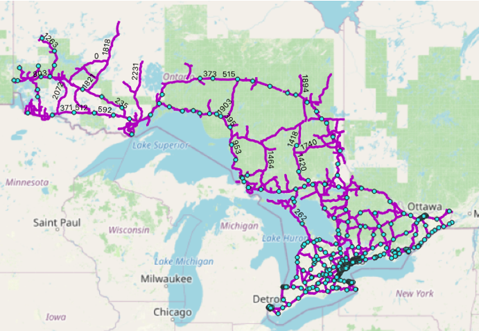
Description for Figure 3
A map featuring the province of Ontario with a layer of purple lines and blue dots over the map. The purple lines represent road segments with available average daily traffic volume annual average daily traffic data, and the blue dots represent Ontario traffic camera locations.
Sources: Authors’ visualization.
AADT from previous years can be combined with counts obtained using traffic imagery to estimate traffic volume for road segments. This can provide a good estimate of traffic for a specific period of the year. The disadvantage of this approach is that the AADT could be significantly different from one year to another, which introduces some inaccuracy to the produced estimates. The approach can be summarized as follows:
Given the daily count from cameras for a road segment, i.e., Nd,c, find the average daily count, Nc, over the period when the counts are available
(1)
By multiplying the normalized daily count, with the historical AADT, NAADT, the estimated daily traffic volume, Nd,est, is given as
(2)
4.2 Model-based approach
With this approach, a model is trained to take the average vehicle count per image over a certain period and outputs the traffic volume for that period. This approach can be summarized in three main steps. In the first step, data are collected (from videos) on average number of vehicles in an image and corresponding traffic volume for a sample period when the images were taken. To do that, images are collected from each video (e.g., 12 images per period Ti, e.g., one minute). Then, the average number of vehicles per image for every sample period Ti is counted. This is followed by finding the ground truth traffic volume for every sample period Ti, i.e., VTi. The second step is to build a model (e.g., linear, polynomial) that maps the average vehicle count to traffic volume for the video period, T. The third step is to use the model to estimate the traffic for any period. Once a model is built, it can be used to estimate the traffic volume for a period P that is M multiple of T. To do this, traffic images over the period P are collected, and then the average number of vehicles per image, NP,avg, is calculated. Afterward, the number of vehicles per T, VT, is estimated using the model. Finally, the number of vehicles per P, i.e., traffic volume for P, is estimated using the following formula:
(3)
4.3 Proposed formula
We propose another approach that eliminates the need for historical data. With this approach, the traffic volume over any duration T can be computed as
(4)
where Navg is the average number of cars per traffic image and Tpass is the average duration for a car to pass through the area in the image. Navg is calculated from static images that are collected during the duration T. An object detection model can be used to detect the number of vehicles in each image to calculate Navg. It is more challenging to compute Tpass because it represents the time it takes a vehicle to pass through the range of view of the traffic camera, so accurate estimation of such duration requires an analysis of a video feed. However, a rough estimate of the period can be made based on an analysis of images from the traffic camera and an estimate or assumption of average speed on that road segment. For example, consider a case where Navg = 6 and Tpass = 2.5s, the estimated traffic volume per minute would be vehicles per minute.
The variables of the formula are illustrated in Figure 4. The figure shows the range of view of a camera on a road. There are two cars that pass through, and it takes the cars Tpass,1 and Tpass,2 seconds to pass through the range of view of the camera. At time t, the number of the cars that would be in an image is Nt = 2.
Figure 4. Illustration of the prediction formula
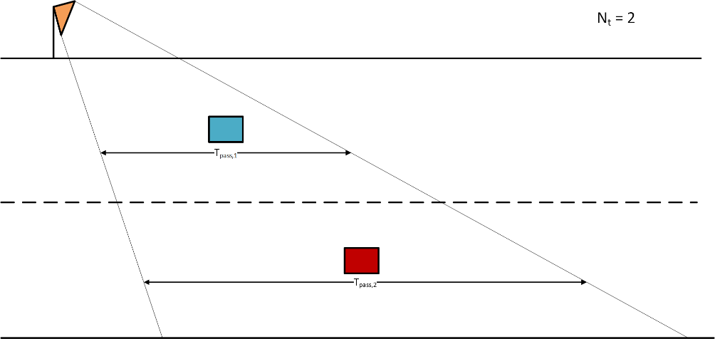
Description for Figure 4
An illustration of a roadway to demonstrate how the prediction formula works. An orange triangle represents a traffic camera, and the lines extending from this triangle show the range of view. A blue rectangle and a red rectangle represent two cars. It takes the blue car Tpass,1 seconds and the red car Tpass,2 seconds to pass through the range of view of the camera. At time t, the number of cars that would be in an image is Nt = 2.
Sources: Authors’ image.
5 Results
5.1 Image samples
Examples of vehicle detection results produced by the system are presented in this section. Figure 5 a) shows a City of Calgary traffic camera image before vehicle detection. Figure 5 b) shows the same image after detection. Both cars and trucks were detected and correctly classified. The vehicles along the visible highway were detected, including the partially visible vehicles at the bottom of the image.
Figure 5. Roadway in Calgary a) before vehicle detection and b) after detection
Detected cars are surrounded by blue bounding boxes and the trucks are surrounded by green bounding boxes.

Description for Figure 5
Two traffic camera images from Calgary are shown to compare (a) an image before vehicle detection occurs and (b) an image after vehicle detection occurs. In image (a), a highway with multiple cars is shown. In image (b), the same highway with cars is shown with coloured rectangles (bounding boxes) and text around the vehicles. Blue rectangles have the text “car” above them, and green rectangles have the text “truck” above them.
Sources: The City of Calgary (Calgary, 2021).
The model was also tested around commercial buildings in Calgary. Figure 6 a) displays a Calgary traffic camera image before object detection. Figure 6 b) shows the same image after detection. All three pedestrians that appear in the image were detected.
Figure 6. Example of detecting pedestrians in the city of Calgary a) before object detection and b) after object detection
Three pedestrians are surrounded by red bounding boxes, and cars are surrounded by blue boxes.
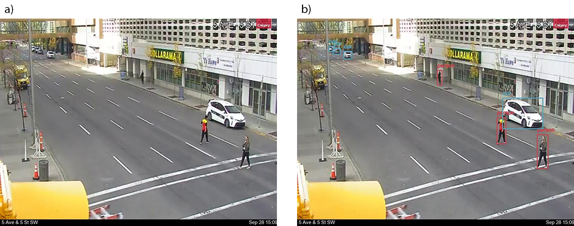
Description for Figure 6
Two traffic camera images from Calgary are shown to compare (a) before pedestrian detection occurs and (b) after pedestrian detection occurs. In image (a), a street is shown with a few cars and two pedestrians crossing the road. In image (b), the same location is shown, with coloured rectangles (bounding boxes) and text around the pedestrians and vehicles. Blue rectangles have the text “car” above them, and red rectangles have the text “person” above them.
Sources: The City of Calgary (Calgary, 2021).
5.2 Analysis of traffic-count data
The data processing model generates insightful traffic trend overviews. The output data were analyzed as a time series and results were visualized. This generated clear traffic patterns and trends which were correlated to typical traffic patterns, such as rush hours, as well as unique events, like lockdowns, restrictions.
Figure 7 shows how Alberta’s COVID-19 prevention lockdown affected traffic. Beginning at 11:59 p.m., February 8, 2022, Alberta began Step 1 of lifting lockdown restrictions (Government of Alberta, 2022) . Step 1 included lifting capacity limits for venues with a capacity of under 500 people, and allowing food and beverage consumption for large events and venues (Government of Alberta, 2022) . The impact on a selected location in Calgary is visible in Figure 7. This location is at a downtown intersection of the city, surrounded by high-rise commercial buildings.
During the first Friday of the lockdown, traffic volume was low. The next Friday—the week Alberta began Step 1—there was a noticeable difference, as car counts increased from about 250 to 3,000. The following week, on Friday, February 18, car counts rose again to about 3,000. Overall, there is an observable trend of traffic recovery after restrictions were eased.
Figure 7. Estimated daily car counts at one selected location (Location #36), Calgary

Description for Figure 7
| Day | Aggregate car count |
|---|---|
| Thur 2022-02-03 | 1,762.55 |
| Fri 2022-02-04 | 2,250.25 |
| Sat 2022-02-05 | 2,532.99 |
| Sun 2022-02-06 | 1,811.43 |
| Mon 2022-02-07 | 2,413.50 |
| Tues 2022-02-08 | 2,566.75 |
| Wed 2022-02-09 | 2,349.49 |
| Thur 2022-02-10 | 2,875.24 |
| Fri 2022-02-11 | 2,252.01 |
| Sat 2022-02-12 | 2,424.94 |
| Sun 2022-02-13 | 1,631.43 |
| Mon 2022-02-14 | 2,597.00 |
| Tues 2022-02-15 | 1,891.69 |
| Wed 2022-02-16 | 1,621.65 |
| Thur 2022-02-17 | 1,862.36 |
| Fri 2022-02-18 | 2,004.65 |
| Sat 2022-02-19 | 2,472.00 |
| Source: Authors’ computations. | |
Figure 8 a) displays aggregate car counts for a weekday in Calgary. There is an increase in car counts around 8:00 a.m., 1:00 p.m. and 5:00 p.m., corresponding to typical rush-hour periods as people commute to work. Figure 8 b) shows the trends based on all camera locations in Calgary during a weekend. Here the increase in traffic counts per hour is much more gradual, compared with weekday hourly traffic, which had rush hour traffic spikes. In the case of Figure 8b, there is a steady increase in traffic between 6:00 a.m. and 2:00 p.m.
Figure 8. a) Car count estimates at a selected location (Location #13) in Calgary, Wednesday, September 22, 2021, and b) hourly car traffic for all traffic cameras in Calgary, Saturday, September 25, 2021
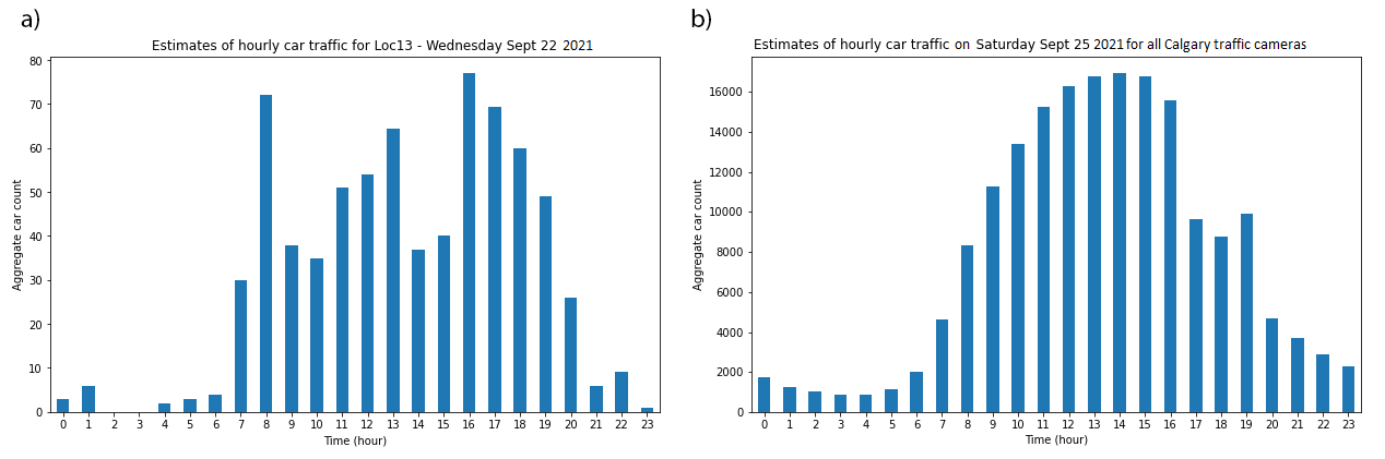
Description for Figure 8
a)
| Time (hour) | Aggregate car count |
|---|---|
| 0 | 3.00 |
| 1 | 6.00 |
| 2 | 0.00 |
| 3 | 0.00 |
| 4 | 2.00 |
| 5 | 3.00 |
| 6 | 4.00 |
| 7 | 30.00 |
| 8 | 72.00 |
| 9 | 38.00 |
| 10 | 35.00 |
| 11 | 51.00 |
| 12 | 54.00 |
| 13 | 64.36 |
| 14 | 37.00 |
| 15 | 40.00 |
| 16 | 77.00 |
| 17 | 69.33 |
| 18 | 60.00 |
| 19 | 49.00 |
| 20 | 26.00 |
| 21 | 6.00 |
| 22 | 9.00 |
| 23 | 1.00 |
| Source: Authors’ computations. | |
b)
| Time(hour) | Aggregate car count |
|---|---|
| 0 | 1,740 |
| 1 | 1,277 |
| 2 | 1,011 |
| 3 | 888 |
| 4 | 878 |
| 5 | 1,165 |
| 6 | 2,012 |
| 7 | 4,647 |
| 8 | 8,330 |
| 9 | 11,286 |
| 10 | 13,379 |
| 11 | 15,251 |
| 12 | 16,272 |
| 13 | 16,759 |
| 14 | 16,923 |
| 15 | 16,794 |
| 16 | 15,583 |
| 17 | 9,659 |
| 18 | 8,786 |
| 19 | 9,929 |
| 20 | 4,683 |
| 21 | 3,679 |
| 22 | 2,899 |
| 23 | 2,309 |
| Source: Authors’ computations. | |
Data can also be aggregated in different ways to gain a multitude of insights. For example, when aggregating Calgary car counts across sites by day of the week for September 22 to September 28, 2021, Wednesday had the highest counts, while Sunday had the lowest.
Analysis on Toronto and Ontario highways was also conducted. Figure 9 a) displays the hourly aggregate car counts for the intersection of Dufferin and Bloor Street in Toronto, during the weekday. This location is surrounded by a subway transit stop and many small shops. As anticipated, most traffic occurs during the workday (between 8:00 a.m. and 4:59 p.m.), peaking around 1:00 p.m., which corresponds to a typical lunch hour. Figure 9 b) shows hourly car traffic around the intersection of Bloor and Bay Street in Toronto during a weekend. This area is surrounded by financial institutions and store outlets. Vehicle traffic picks up in the morning here and remains steady, except for a dip between 5:00 and 6:00 p.m. Traffic also decreases later and more gradually, compared with the previous example.
Figure 9. a) Hourly car traffic at Toronto’s Dufferin and Bloor Street intersection (Location #8049), Wednesday, December 8, 2021, and b) hourly car traffic at Toronto’s Bay and Bloor Street intersection (Location #8043), Saturday, December 11, 2021

Description for Figure 9
a)
| Time (hour) | Aggregate car count |
|---|---|
| 0 | 4 |
| 1 | 3 |
| 2 | 5 |
| 3 | 1 |
| 4 | 6 |
| 5 | 2 |
| 6 | 5 |
| 7 | 16 |
| 8 | 39 |
| 9 | 34 |
| 10 | 36 |
| 11 | 33 |
| 12 | 34 |
| 13 | 44 |
| 14 | 43 |
| 15 | 41 |
| 16 | 32 |
| 17 | 7 |
| 18 | 13 |
| 19 | 16 |
| 20 | 13 |
| 21 | 13 |
| 22 | 14 |
| 23 | 10 |
| Source: Authors’ computations. | |
b)
| Time (hour) | Aggregate car count |
|---|---|
| 0 | 5 |
| 1 | 7 |
| 2 | 1 |
| 3 | 5 |
| 4 | 3 |
| 5 | 3 |
| 6 | 3 |
| 7 | 14 |
| 8 | 19 |
| 9 | 26 |
| 10 | 16 |
| 11 | 20 |
| 12 | 24 |
| 13 | 23 |
| 14 | 14 |
| 15 | 19 |
| 16 | 25 |
| 17 | 5 |
| 18 | 18 |
| 19 | 13 |
| 20 | 12 |
| 21 | 7 |
| 22 | 6 |
| 23 | 6 |
| Source: Authors’ computations. | |
Traffic data for provincial Ontario highways were also collected (see Figure 10). Both a cyclical pattern and a gradual decrease in traffic occurs for December. The gradual reduction in traffic likely reflects the reduced need to travel for work during the holiday break. The dips in traffic counts correspond to the weekend, also likely reflecting fewer people using the highway for work.
Figure 10. Estimates of daily car traffic for an Ontario highway camera (Location #23-3) for December 2021
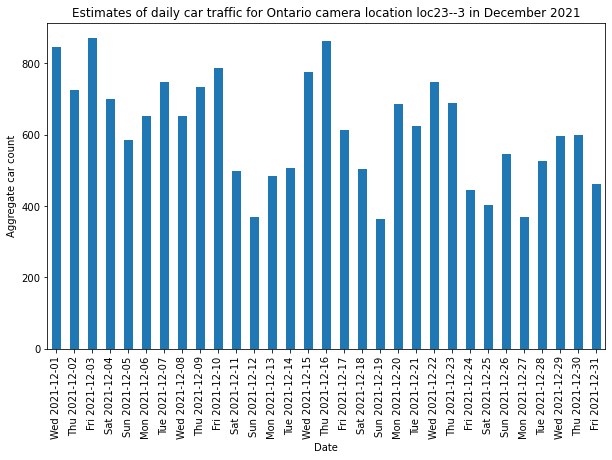
Description for Figure 10
| Date | Aggregate Car Count |
|---|---|
| Wed 2021-12-01 | 845 |
| Thu 2021-12-02 | 726 |
| Fri 2021-12-03 | 871 |
| Sat 2021-12-04 | 699 |
| Sun 2021-12-05 | 584 |
| Mon 2021-12-06 | 653 |
| Tue 2021-12-07 | 749 |
| Wed 2021-12-08 | 652 |
| Thu 2021-12-09 | 733 |
| Fri 2021-12-10 | 787 |
| Sat 2021-12-11 | 499 |
| Sun 2021-12-12 | 368 |
| Mon 2021-12-13 | 484 |
| Tue 2021-12-14 | 508 |
| Wed 2021-12-15 | 776 |
| Thu 2021-12-16 | 862 |
| Fri 2021-12-17 | 613 |
| Sat 2021-12-18 | 505 |
| Sun 2021-12-19 | 363 |
| Mon 2021-12-20 | 685 |
| Tue 2021-12-21 | 624 |
| Wed 2021-12-22 | 747 |
| Thu 2021-12-23 | 689 |
| Fri 2021-12-24 | 446 |
| Sat 2021-12-25 | 403 |
| Sun 2021-12-26 | 545 |
| Mon 2021-12-27 | 370 |
| Tue 2021-12-28 | 525 |
| Wed 2021-12-29 | 595 |
| Thu 2021-12-30 | 600 |
| Fri 2021-12-31 | 461 |
| Source: Authors’ computations. | |
5.3 Traffic volume estimation
In this section, we show results obtained from the proposed approaches for traffic volume estimation. Figure 11 shows the AADT-based daily traffic volume estimates for a highway in Ontario (Queen Elizabeth Way between Bronte Road and Third Line) for the month of December 2021. The figure shows that the highest daily traffic volume value is 32,0662, on December 23, 2021. This can be explained by the typically higher mobility volume related to holiday events and travel to major shopping centres before Christmas. The lowest daily traffic values are on December 25, 2021 (Christmas Day) and December 27, 2021, i.e., the day after Boxing Day. December 27 was a statutory holiday in Ontario because Christmas Day fell on a Saturday, which explains the low traffic volume on both days. The increase in traffic volume on December 26 was because of Boxing Day, when people go out to shop or for social interactions.
Figure 11. Estimates of daily traffic volume on an Ontario highway segment
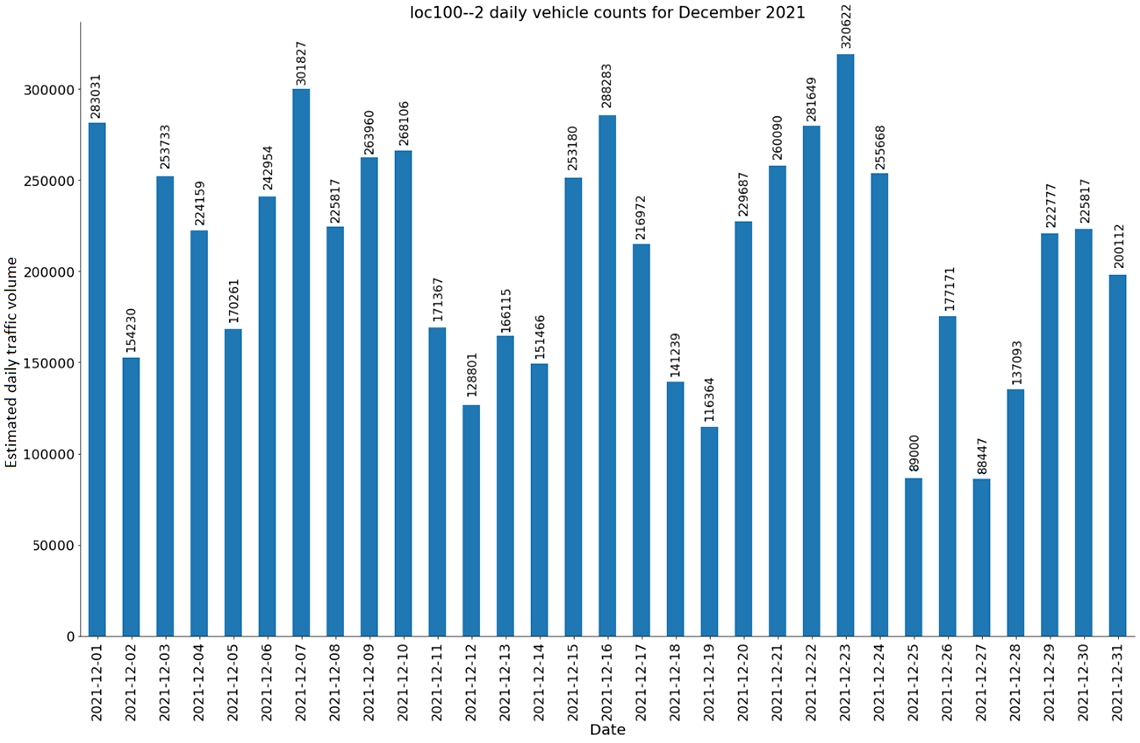
Description for Figure 11
| Date | Estimated daily traffic volume |
|---|---|
| 2021-12-01 | 283,031 |
| 2021-12-02 | 154,230 |
| 2021-12-03 | 253,733 |
| 2021-12-04 | 224,159 |
| 2021-12-05 | 170,261 |
| 2021-12-06 | 242,954 |
| 2021-12-07 | 301,827 |
| 2021-12-08 | 225,817 |
| 2021-12-09 | 263,960 |
| 2021-12-10 | 268,106 |
| 2021-12-11 | 171,367 |
| 2021-12-12 | 128,801 |
| 2021-12-13 | 166,115 |
| 2021-12-14 | 151,466 |
| 2021-12-15 | 253,180 |
| 2021-12-16 | 288,283 |
| 2021-12-17 | 216,972 |
| 2021-12-18 | 141,239 |
| 2021-12-19 | 116,364 |
| 2021-12-20 | 229,687 |
| 2021-12-21 | 260,090 |
| 2021-12-22 | 281,649 |
| 2021-12-23 | 320,622 |
| 2021-12-24 | 255,668 |
| 2021-12-25 | 89,000 |
| 2021-12-26 | 177,171 |
| 2021-12-27 | 88,447 |
| 2021-12-28 | 137,093 |
| 2021-12-29 | 222,777 |
| 2021-12-30 | 225,817 |
| 2021-12-31 | 200,112 |
| Source: Authors’ computations. | |
Figure 12 shows the results obtained from both the AADT-based approach and model-based approach. Although the estimates from both approaches follow the same trend, those obtained from the model-based approach are significantly lower than those obtained from the AADT-based approach. This may be caused by the following reasons:
- The AADT value used is from 2016, before the pandemic, while traffic has dropped since 2020 because of lockdowns and teleworking.
- The model was built using videos from roads with different characteristics, i.e., two directions with two lanes each, while the test images were from a highway with three lanes in each direction.
- The model was built using ground truth vehicle counts, while estimations used counts of detected vehicles that are expected to be lower.
Unfortunately, we did not have a road segment with both historical data and recent video data that could be used to collect ground truth traffic volumes to validate the proposed models. We are currently looking for such data to validate the proposed methods.
Figure 12. Comparison of model-based and annual average daily traffic-based daily traffic volume estimations
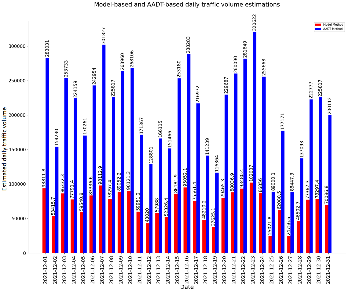
Description for Figure 12
| Date | Estimated daily traffic volume - model method | Estimated daily traffic volume - AADT method |
|---|---|---|
| 2021-12-01 | 93,811.82 | 283,031.46 |
| 2021-12-02 | 53,415.68 | 154,230.03 |
| 2021-12-03 | 86,332.32 | 253,733.28 |
| 2021-12-04 | 77,791.43 | 224,158.71 |
| 2021-12-05 | 59,540.78 | 170,261.11 |
| 2021-12-06 | 83,336.58 | 242,953.76 |
| 2021-12-07 | 98,112.93 | 301,826.52 |
| 2021-12-08 | 78,297.36 | 225,817.09 |
| 2021-12-09 | 89,052.16 | 263,960.01 |
| 2021-12-10 | 90,121.26 | 268,105.97 |
| 2021-12-11 | 59,951.18 | 171,366.70 |
| 2021-12-12 | 43,020.00 | 128,801.43 |
| 2021-12-13 | 57,988.03 | 166,115.14 |
| 2021-12-14 | 52,326.42 | 151,466.06 |
| 2021-12-15 | 86,181.92 | 253,180.49 |
| 2021-12-16 | 95,052.11 | 288,283.02 |
| 2021-12-17 | 75,561.43 | 216,972.36 |
| 2021-12-18 | 48,210.22 | 141,239.33 |
| 2021-12-19 | 37,625.09 | 116,363.52 |
| 2021-12-20 | 79,465.25 | 229,686.66 |
| 2021-12-21 | 88,036.93 | 260,090.43 |
| 2021-12-22 | 93,480.42 | 281,649.47 |
| 2021-12-23 | 102,037.21 | 320,621.58 |
| 2021-12-24 | 86,855.96 | 255,668.07 |
| 2021-12-25 | 25,021.78 | 89,000.13 |
| 2021-12-26 | 62,080.55 | 177,171.06 |
| 2021-12-27 | 24,756.60 | 88,447.33 |
| 2021-12-28 | 46,502.71 | 137,093.36 |
| 2021-12-29 | 77,367.34 | 222,776.72 |
| 2021-12-30 | 78,297.36 | 225,817.09 |
| 2021-12-31 | 70,086.81 | 200,112.09 |
| Source: Authors’ computations. | ||
Figure 13 shows the ratio of the model-based estimate to the AADT-based estimate. The ratio falls in the range of 0.28 to 0.35, which means it is consistent.
Figure 13. Ratio of the annual average daily traffic-based estimates to model-based estimates

Description for Figure 13
| Date | Model-AADT-based estimation ratio |
|---|---|
| 2021-12-01 | 0.3315 |
| 2021-12-02 | 0.3463 |
| 2021-12-03 | 0.3402 |
| 2021-12-04 | 0.3470 |
| 2021-12-05 | 0.3497 |
| 2021-12-06 | 0.3430 |
| 2021-12-07 | 0.3251 |
| 2021-12-08 | 0.3467 |
| 2021-12-09 | 0.3374 |
| 2021-12-10 | 0.3361 |
| 2021-12-11 | 0.3498 |
| 2021-12-12 | 0.3340 |
| 2021-12-13 | 0.3491 |
| 2021-12-14 | 0.3455 |
| 2021-12-15 | 0.3404 |
| 2021-12-16 | 0.3297 |
| 2021-12-17 | 0.3483 |
| 2021-12-18 | 0.3413 |
| 2021-12-19 | 0.3233 |
| 2021-12-20 | 0.3460 |
| 2021-12-21 | 0.3385 |
| 2021-12-22 | 0.3319 |
| 2021-12-23 | 0.3182 |
| 2021-12-24 | 0.3397 |
| 2021-12-25 | 0.2811 |
| 2021-12-26 | 0.3504 |
| 2021-12-27 | 0.2799 |
| 2021-12-28 | 0.3392 |
| 2021-12-29 | 0.3473 |
| 2021-12-30 | 0.3467 |
| 2021-12-31 | 0.3502 |
| Source: Authors’ computations. | |
In the following application, the results obtained with the proposed formula are discussed. Here, a traffic video is used to manually count cars in the video to find the ground-truth traffic volume during different sample periods (of one minute each in length) of the video. The parameters Navg and Tpass for those periods are also determined. Recall that the proposed formula to estimate traffic volume over a given period, T, is given in (4). For this, Navg and Tpass must be estimated. Navg is the average number of vehicles detected in an image. To estimate Navg for a sample period, images were collected from different times (e.g., every 10 seconds) during the video for each period, and the number of vehicles in each image was counted. The number of vehicles in an image taken from the video at time t is referred to as Nt. Tpass,i is the duration for a vehicle, i, to pass across the camera range of view for different cars. For each sample period, the value of Tpass,i was collected for different vehicles. Then, for each period (of one minute), the average of the different values of Nt was calculated to find the value of Navg, and the average value of Tpass,i was calculated to find Tpass.
In addition to the above, a computer vision model was used to detect vehicles in an area of interest in the video and record the time they enter and leave that area. These data were also used to estimate Navg and Tpass. To sum up, the following data were collected for multiple one-minute periods:
- actual traffic volume for each sample period
- Navg and Tpass based on manual data collection for each period (used to estimate traffic volume for that period)
- Navg and Tpass collected by a vehicle-detection model for each period (used to estimate traffic volume for that period)
The results obtained from this experiment are shown in Figure 14, with three curves that depict the estimated traffic volume for each period. Each curve corresponds to one of the approaches above. Because the results obtained from the three methods are close, this suggests that the proposed formula can be used to provide accurate estimates of traffic volume. The only missing information for this system is Tpass, which is difficult to obtain from static images. However, the value can be estimated using visual investigation of images of the road segment.
Figure 14. Comparison of the results from three volume estimation methods

Description for Figure 14
| Time (min) | Proposed formula with manual count | Manual count | Proposed formula with CV model |
|---|---|---|---|
| Volume (vehicles/5 min) | |||
| 1 | 417 | 459 | 394 |
| 2 | 374 | 415 | 336 |
| 3 | 313 | 362 | 330 |
| 4 | 398 | 425 | 375 |
| 5 | 290 | 334 | 276 |
| 6 | 429 | 436 | 352 |
| Source: Authors’ computations. | |||
6 Conclusion and future work
In this paper, a computer vision-based system has been presented that was developed to periodically extract vehicle counts from Canadian traffic camera imagery. First, a study was conducted to compile data on available traffic camera programs in Canada. Then, a system was developed to collect imagery from multiple APIs available through three traffic camera programs (the cities of Calgary and Toronto, and the province of Ontario). The system detects different types of vehicles in these images using the open-source YOLOv3 object detection model that was trained on the COCO dataset. Furthermore, counts of the detected vehicle types (car, bus, motorcycle, etc.) were generated. The results produced were exported as a time series, and analysis was conducted on the extracted data. Visualization and analysis of the collected datasets show that clear traffic patterns and trends can be seen. Different methods were proposed for estimating traffic volume from counts obtained from the static images. The proposed methods were used with collected count data to estimate the traffic volume of multiple road segments.
It was observed that some of the traffic camera APIs are better than others, in terms of image quality and availability. For example, the camera images from Calgary are more reliable and have fewer outages than those from Toronto. If a continuous data stream is to be collected by the system, a reliable host (e.g., local server or cloud environment) will be required. The system is currently deployed on the Statistics Canada cloud environment, the Advanced Analytics Workspace, where a separate instance is running for each API on a different notebook server.
As mentioned at the outset, monitoring traffic in large urban regions is an important function, particularly with increasing congestion and policy implications ranging from the cost of time to carbon emissions. A key element of traffic monitoring is vehicular counts, and this research proposes a novel approach by using traffic cameras. The results of the image processing workflow show clear traffic trends and patterns throughout the day and week, with data correlating to unique events, such as lockdowns, restrictions and holidays. These datasets have multiple uses, ranging from providing basic traffic counts to producing comprehensive indexes of local economic activities. This information can also be used to supplement existing data sources on mobility in tourism and transportation programs.
Several model refinements are possible. For instance, exploratory work is currently being conducted to train a model that can classify commercial trucks (e.g., trailer trucks, box trucks, tankers, chiller trucks), as this can provide an indication of economic activities. Specifically, those from road segments on provincial borders would be particularly important. Moreover, the extracted datasets inside municipal areas will be used to create indicators on mobility, which can be used in indexes on local business conditions. Furthermore, analysis of datasets for certain touristic districts will be conducted to measure activity in such areas. Finally, further development will be implemented on the workflow to automate the whole process from data collection until analysis and visualization to produce real-time traffic data on a daily or weekly basis.
References
Calgary, T. C. (2021). Calgary Traffic Cameras. Retrieved from Calgary.ca: https://trafficcam.calgary.ca
Chen, L., Grimstead, I., Bell, D., Karanka, J., Dimond, L., James, P., . . . & Edwardes, A. (2021). Estimating Vehicle and Pedestrian Activity from Town and City Traffic Cameras. Basel.
City of Calgary. (2022, March). Calgary Traffic Cameras. Retrieved from Calgary.ca: https://www.calgary.ca/transportation/roads/traffic/advisories-closures-and-detours/calgary-traffic-cameras.html
COMPASS/Ministry of Transportation. (2021). Retrieved from 511 Ontario: https://511on.ca
Cordts, M., Omran, M., Ramos, S., Rehfeld, T., Enzweiler, M., Benenson, R., . . . Schiele, B. (2019). Cityscapes dataset. Retrieved from https://www.cityscapes-dataset.com/
Doulamis, N., Doulamis, A., & Protopapadakis, E. (2018). Deep Learning for Computer Vision: A Brief Review. Computational Intelligence and Neuroscience.
Ecola, L., & Wachs, M. (2012). Exploring the Relationship between Travel Demand and Economic Growth. The RAND Corporation. Retrieved from https://www.fhwa.dot.gov/policy/otps/pubs/vmt_gdp/index.cfm
Fedorov, A., Nikolskaia, K., Ivanov, S., Shepelev, V., & Minbaleev, A. (2019). Traffic flow estimation with data from a video surveillance camera. Journal of big data.
Government of Alberta. (2022, February 8). Alberta takes steps to safely return to normal | L’Alberta prend des mesures pour un retour à la normale sécuritaire. Retrieved from Alberta.ca: https://www.alberta.ca/release.cfm?xID=8185996876395-A336-5B57-A82D6FEE916E1060
Li, S., Chang, F., Liu, C., & Li, N. (2020). Vehicle counting and traffic flow parameter estimation for dense traffic scenes. IET Intelligent Transport Systems.
Lin, T.-Y., Maire, M., Belongie, S., Hays, J., Perona, P., Ramanan, D., . . . Zitnick, C. L. (2014). Microsoft COCO: Common Objects in Context. European Conference on Computer Vision, (pp. 740-755).
Liu, J., Weinert, A., & Amin, S. (2018). Semantic topic analysis of traffic camera images. IEEE.
Liu, W., Anguelov, D., Erhan, D., Szegedy, C., Reed, S., Fu, C.-Y., & Berg, A. C. (2016). SSD: Single Shot MultiBox Detector. European Conference on Computer Vision, (pp. 21-37).
Redmon, J. (2018). YOLO: Real-Time Object Detection. Retrieved from https://pjreddie.com/darknet/yolo/
Redmon, J., & Farhadi, A. (2018). YOLOv3: An Incremental Improvement. arXiv: 1804.02767.
Ren, S., He, K., Girshick, R., & Sun, J. (2016). Faster R-CNN: Towards Real-Time Object Detection with Region Proposal Networks.
Schrank, D., Eisele, B., & Lomax, T. (2019). 2019 Urban Mobility Report. The Texas A&M Transportation Institute.
Sekułaa, P., Markovića, N., Laana, Z. V., & Sadabadia, K. F. (2018). Estimating historical hourly traffic volumes via machine learning and vehicle probe data: A Maryland case study. Transportation Research Part C: Emerging Technologies, 97, 147-158.
Snowdon, J., Gkountouna, O., Zü e, A., & Pfoser, D. (2018). Spatiotemporal Traffic Volume Estimation Model Based on GPS Samples. Proceedings of the Fifth International ACM SIGMOD Workshop on Managing and Mining Enriched Geo-Spatial, (pp. 1-6).
Song, H., Liang, H., Li, H., Dai, Z., & Yun, X. (2019). Vision-based vehicle detection and counting system using deep learning in highway scenes. European Transport Research Review.
Yadav, P., Sarkar, D., Salwala, D., & Curry, E. (2020). Traffic prediction framework for OpenStreetMap using deep learning based complex event processing and open traffic cameras. arXiv preprint arXiv:2008.00928.
Yang, H., Yang, J., Han, L., Liu, X., Pu, L., Chin, S.-M., & Hwang, H.-L. (2018). A Kriging based spatiotemporal approach for traffic volume data imputation. Public Library of Science.
Zhao, X., Carling, K., & Håkansson, J. (2014). Reliability of GPS based traffic data: an experimental evaluation.
- Date modified: