
Reports on Special Business Projects
The Impact of Business Innovation and Growth Support on Employment and Revenue of Manufacturing Enterprises, 1 to 3 Years After Receipt of Support

Archived Content
Information identified as archived is provided for reference, research or recordkeeping purposes. It is not subject to the Government of Canada Web Standards and has not been altered or updated since it was archived. Please "contact us" to request a format other than those available.
Skip to text
Acknowledgements
I would like to thank Sylvain Ouellet, Mahamat Hamit-Haggar and Julio Rosa for their support and comments throughout the development of this analytical report. I am also grateful to Nathalie Brault, Alessandro Alasia and Jeffrey Smith for their suggestions and comments.
I would like to acknowledge the assistance of my colleagues at the Centre for Special Business Projects and the Treasury Board of Canada Secretariat as well as the comments provided by external reviewers. I would like to express special thanks to Sarah Feng, Alexander Davies, Peter Timusk, Esteban Pinzon-Delgado, Ian Gibson, Abdulkadir Musa and Daouda Sylla.
Summary
The federal government offers business innovation and growth support through program streams managed by its departments and agencies. In 2017, enterprises in the manufacturing sector accounted for almost one-quarter of the beneficiaries of this support and received almost one-third of the total value of support (Statistics Canada, 2020). The objective of this analysis is to assess the impact of federal growth and innovation support on the employment and revenue of beneficiary enterprises in the manufacturing sector between 2007 and 2017. This analysis suggests that enterprises that received federal support for growth and innovation experienced stronger employment and revenue growth relative to non-beneficiary enterprises. Over the three years following receipt of support, employment growth for beneficiary enterprises averaged 1.8% per year while, on average, enterprises that did not receive support experienced employment declines. Over the same period, the average annual revenue growth of beneficiary enterprises was higher than that of non-beneficiary enterprises by 4.6 percentage points.
Introduction
In Budget 2018, the Government of Canada announced funding for Statistics Canada to improve performance evaluations of programs related to business innovation and growth support (BIGS). Following this announcement, Statistics Canada’s Centre for Special Business Projects acquired administrative data on support for business innovation and growth offered through the program streams of 18 federal departments and agencies for the period from 2007 to 2017. These administrative data were subsequently linked to Statistics Canada’s Business Register (BR) and Linkable File Environment (LFE)to create a database of beneficiaries of support from business innovation and growth program streams.
The objective of the BIGS statistical program is to contribute to improving performance evaluations and impact assessments of the growth and innovation program streams, as announced in the 2018 federal budget. This analysis considers all federal program streams providing support to enterprises between 2007 and 2017.
More specifically, this analysis focuses on beneficiary enterprises in a specific sector of the economy, the manufacturing sector, regardless of the program stream. In Canada, the economy can be divided into 20 sectors according to the North American Industry Classification System (NAICS). The manufacturing sector comprises establishments primarily engaged in the chemical, mechanical or physical transformation of materials or substances into new products (Statistics Canada, 2018). An analysis of the distribution of support by economic sector showed that, in 2017, the manufacturing sector accounted for almost one-quarter (24.4%) of all enterprises receiving federal innovation and growth support and received almost one-third (32.1%) of the total value of support (Statistics Canada, 2020).
Few studies looked at the impact of support programs on manufacturing businesses in particular. This report presents the first analysis on manufacturing businesses using BIGS data. The objective of this analysis is to assess the impact of federal support for growth and innovation on enterprises in the manufacturing sector that received support between 2007 and 2017. Based on the proven nonparametric approach of the propensity score (Rosenbaum and Rubin, 1983), this study presents the following research question: Did the program streams associated with business innovation and growth support have an impact on the performance of manufacturing enterprises between 2007 and 2017?Note
Literature review
Some research suggests that national business support programs are associated with positive employment growth.
Canadian studies
Belleau-Arsenault (2017) studied the impact of government financial aids on employment growth and survival of businesses located in Quebec’s Bas-Saint-Laurent region and from several sectors including the manufacturing sector. Using data on government financial aids offered between 2006 and 2015, this study showed that government support had a positive effect on enterprises’ employment growth, and this effect was especially pronounced for enterprises in the manufacturing sector compared with enterprises in the primary and tertiary sectors (Belleau-Arsenault, 2017).
An impact study of the Canada Small Business Financing Program showed that beneficiary enterprises experienced a higher revenue and employment growth of 6 and 3 percentage points respectively between 2014 and 2016 compared to non-beneficiary enterprises (Huang and Rivard, 2019).
An internal analysis at Innovation, Science and Economic Development Canada supported the idea that enterprises receiving both tax credits and direct research and development (R&D) grants performed better than enterprises receiving only R&D tax credits (Bérubé and Therrien, 2016). In this study of Canadian enterprises receiving R&D tax credits between 2000 and 2007, employment, sales, wages and profit were significantly higher for enterprises receiving direct and indirect incentives compared with enterprises receiving only indirect incentives, three and five years after receiving support.
International studies
Vanino et al. (2019) conducted an impact study of enterprises receiving innovation and R&D grants in the United Kingdom between 2004 and 2016. The results show that grants have a positive effect on employment and sales growth, especially for beneficiary enterprises in the manufacturing sector, over a two- and five-year horizon. This positive impact of financial assistance on employment and sales appears to be greater for smaller enterprises, such as those with 250 or fewer employees, than for enterprises with more than 250 employees.
An evaluation of the impact of support for small- and medium-sized business in Europe between 2005 and 2012 found that, on average, the program had a positive impact on the employment of the enterprises (Asdrubali et al., 2015). The support program increased employment of beneficiary enterprises by an average of 17.3% over 5 years, compared with non-beneficiary enterprises. The program also increased the sales of beneficiary enterprises by an average of 19.6% over 5 years compared with non-beneficiaries.
In a study of the impact of grants on Italian enterprises between 2000 and 2009, Biagi et al. (2015) found that financial assistance created, on average, almost two new jobs per beneficiary enterprise. Grants increased the number of jobs per enterprise by an average of 1.91 jobs for enterprises in the manufacturing sector compared with an average increase of 1.45 jobs for those in the services sector.
Data
This study is produced using the linkage between two separate data sources. On the one hand, this study is based on the business innovation and growth support (BIGS) database which covers government activities that support business innovation and growth, such as funding, business consulting services, and support provided directly, through an intermediary or in partnership. It covers the period from 2007 to 2017 and contains the identifier of the statistical enterpriseNote beneficiary of support, the value of support received, the year and type of support as well as the department and program stream providing the support. On the other hand, this study uses data from the Linkable File Environment (LFE) from 2006 to 2018, which covers enterprise-level information such as location, annual operating revenue, average annual number of employees, etc. The main data sources for the LFE used in this analysis are the Business Register, the Corporate Revenue Tax File (T2), the Statement of Account for Current Source Deductions (PD7)Note and Statistics Canada’s Chart of Accounts.
This study is based only on enterprises that were matched to the BR. The database match rate to the BR is over 95%. There may be several reasons why some records could not be linked, including
- a beneficiary has recently been added to the BR but has not yet been assigned to a NAICS sector
- an enterprise’s recent administrative changes are not yet in the BR
- an enterprise may exist in the BR but under a different name than that acquired in the administrative data
- the business name received from the federal department or agency was incomplete.
Given the high match rate obtained, the impact of records that could not be matched on the accuracy of the estimates from this analysis is negligible.
This impact assessment considers ultimate beneficiariesNote of program streams identified in the inventory of federal BIGS program streams before the BIGS administrative data acquisitionNote .
This study considers only the year of receipt of the initial supportNote . Although, beneficiary enterprises in the manufacturing sector may have received support from more than one program stream, more than one type of support (e.g., advisory service and grant)Note and in more than one year between 2007 and 2017. Also, the value of the support received by the enterprise is not considered in this assessment which is based on the propensity score matching method for binary treatment. In other words, whether or not support was received is considered in the impact assessment, but not the intensity of the support received.
Methodological approach
Following a brief descriptive analysis, an assessment of the effects of federal support for business innovation and growth on beneficiary enterprises was conducted using the propensity score matching method.
A list of potential enterprises for the control group was identified from the Generic Survey Universe File (GSUF)Note for each year from 2007 to 2017. Potential enterprises were selected if they were classified in the manufacturing sector and did not receive innovation and growth support between 2007 and 2017.
In this analysis, we assessed the multicollinearity among available explanatory variablesNote . The propensity score of treated and potential control group enterprises was then estimated using the following logistic regression model:Note
where, for
- is the number of treated and potential control enterprises
- and if enterprise received federal support and if not
- (Country) indicates whether enterprise ’s country of control is Canada ( ) or not ( )
- (Region) indicates whether the economic region of enterprise is Atlantic ( ), Quebec ( ), Ontario ( ), the Prairies ( ) or British Columbia or the territories ( )
- (MultiProvince) indicates whether enterprise operates in more than one province ( ) or not ( )
- (R&D) indicates whether enterprise reported research and development expenditures ( ) or not ( )
- (NAICS) indicates the North American Industry Classification System code of enterprise
- (Log Age) indicates the log of the age of enterprise
- (Log Employment) indicates the log of the average number of employees in enterprise
- (Log Revenue) indicates the log of the operating revenue of enterprise
- (Log Sales) indicates the log of the total sales of enterprise
- (Log Assets) indicates the log of the total assets of enterprise
- (Log Debt Ratio) indicates the log of the debt ratio (assets/liabilities) of the enterprise.
Once the propensity score has been estimated using the chosen model, the quality is evaluated by comparing the distribution of explanatory variables for beneficiary and potential control group enterprises by propensity score stratum. With a good quality propensity score, the distribution of each explanatory variable should be similar between the treated and potential control groups for each propensity score stratum. The standardized mean difference and the variance ratio are used to compare the distribution of explanatory variables between the treated and potential control groups. For a good quality propensity score, the absolute standardized mean difference should be less than or equal to 0.25 and the variance ratio should be between 0.5 and 2 (Stuart, 2010).
Following estimation of the propensity score, the matching of treated enterprises with potential control enterprises is initially carried out exactly using the reference year and industry subsector, and then probabilistically using propensity score predictions (Burden et al., 2017). The probabilistic matching strategy used in this analysis combines two methods: nearest neighbour matching and caliper matching (Stuart, 2010). Each beneficiary enterprise is matched to a GSUF enterprise in the same reference year and manufacturing subsector so that the difference between their propensity score logits is minimal.
To limit lower quality pairs, the strategy chosen is to accept only pairs in which the difference between the propensity score logits of the treated enterprise and the potential control enterprise is less than or equal to a specific threshold . This threshold considers , the variance of the logit of the propensity scores of the beneficiary enterprises and , the variance of the logit of the propensity scores of the potential control enterprises:
(SAS, 2016).
In other words, if denotes all potential control enterprises for a given year and subsector and is the propensity score logit, then the potential control enterprise that is matched to the treated enterprise is defined by:
Matching results in two groups of the same size: the treated group comprising of enterprises that received federal support for innovation and growth, and the control group comprising of enterprises that did not receive such support. The quality of the match is assessed by comparing, for each covariate, the average value before receiving support in the treated and control groups, before and after matching. Differences observed between the average value in the treated group and the control group before the match should no longer exist after the match, the initial selection bias having been controlled by this technique.
With a good quality matching, any systematic difference between treated and control enterprises prior to receiving support is greatly reduced or fully controlled, and the difference in performance between the two groups after receiving support can be fully attributed to this support. Thus, the average effect of federal support for innovation and growth is estimated by comparing the compound annual growth rate of employment and revenue of beneficiary enterprises with the growth rate of employment and revenue of the control group enterprises with which they are matched.
The compound annual growth rate ( ) for the indicator (employment or revenue in this analysis) of enterprise between year and year is calculated using the following formula:Note
Descriptive results
Between 2007 and 2017, the manufacturing sector had a total of 12,527 enterprises that received federal growth and innovation support (Table 1). The total value of support received by these enterprises during this period exceeded $4.7 billion.
Each year, the manufacturing sector had between 1,221 and 5,213 beneficiary enterprises, and received between $263 million and $602 million in federal support for business innovation and growth (Statistics Canada, Table 33-10-0221-01).
For the period from 2007 to 2017, each beneficiary enterprise in the manufacturing sector received support over an average of 2.9 years (Table 1). Each manufacturing beneficiary enterprise received support from 1.8 program streams on average and 1.6 different types of support on average between 2007 and 2017 (Table 1)
| Value | |
|---|---|
| Number of enterprises | 12,527 |
| Total value of support ($) | 4,707,275,347 |
| Average number of years of support per enterprise | 2.9 |
| Average number of program streams per enterprise | 1.8 |
| Average number of support types per enterprise | 1.6 |
|
|
Over the same period, more than one in two beneficiary manufacturing enterprises (53.3%) received repayable or non-repayable contributions as financial assistance. These contributions accounted for almost 95% of the total value of support to beneficiary enterprises in the manufacturing sector between 2007 and 2017.
| Type of support | Beneficiary enterprises (N=12,527) | Value of support to enterprises | ||
|---|---|---|---|---|
| number | proportion (percent) | thousands of $ | percent | |
| Advisory service | 10,106 | 80.7 | 0 | 0.0 |
| Non-repayable contribution | 4,514 | 36.0 | 1,065,589 | 22.6 |
| Consortium member | 2,509 | 20.0 | 0 | 0.0 |
| Unconditionally repayable contribution | 1,897 | 15.1 | 1,978,970 | 42.0 |
| Grant | 416 | 3.3 | 18,172 | 0.4 |
| Service fully cost-recovered | 380 | 3.0 | 107,006 | 2.3 |
| Conditionally repayable contribution | 273 | 2.2 | 1,425,954 | 30.3 |
| Service partially cost-recovered | 191 | 1.5 | 36,921 | 0.8 |
| Targeted procurement | 91 | 0.7 | 74,662 | 1.6 |
|
||||
Chart 1 shows the proportion of beneficiary enterprises and the proportion of total value of support for the 2007-to-2017 period by manufacturing subsector.Note For example, the transportation equipment manufacturing subsector received more than one-third of the total value of support, although it accounts for only about 6% of the total number of enterprises. The transportation equipment manufacturing subsector and the machinery manufacturing subsector received more than half of the total value of support between 2007 and 2017.Note

Data table for Chart 1
| Subsector | Enterprises | Value of support |
|---|---|---|
| percent | ||
| Food manufacturing | 11.6 | 6.3 |
| Beverage and tobacco product manufacturing | 3.3 | 0.8 |
| Wood product manufacturing | 5.3 | 3.5 |
| Paper manufacturing | 1.1 | 2.5 |
| Chemical manufacturing | 7.1 | 5.9 |
| Plastics and rubber products manufacturing | 5.3 | 2 |
| Fabricated metal product manufacturing | 11.4 | 3.3 |
| Machinery manufacturing | 14.2 | 19 |
| Computer and electronic product manufacturing | 9.5 | 9.5 |
| Electrical equipment, appliance and component manufacturing | 4.5 | 3.4 |
| Transportation equipment manufacturing | 6.1 | 34.3 |
| Furniture and related product manufacturing | 3.5 | 1.1 |
| Miscellaneous manufacturing | 10.8 | 4.2 |
| Other manufacturing subsectors | 9.5 | 4.4 |
| Source: Statistics Canada, Business Innovation and Growth Support. | ||
Chart 2 shows the proportion of beneficiary enterprises in the manufacturing sector and the proportion of the total value of support between 2007 and 2017 by program stream.Note During this period, nearly two-thirds of beneficiary enterprises in the manufacturing sector received support from the Industrial Research Assistance Program, one of the Government of Canada’s largest program streams. These enterprises received more than 10% of the total value of support between 2007 and 2017.
In addition, the Trade Commissioner Service program stream provided advisory services to almost two in five beneficiary manufacturing enterprises over the same period.Note These services were provided at no cost to the client, so the total value of support for this program stream is zero.

Data table for Chart 2
| Program stream | Enterprises | Value of support |
|---|---|---|
| percent | ||
| AgriInnovation Program | 0.3 | 1.9 |
| Commercialization and Exports | 2.1 | 0.8 |
| Productivity and Expansion | 7.2 | 8.4 |
| Applied Research and Development Grants | 3.9 | 0 |
| Collaborative Research and Development Grants | 5.4 | 0 |
| Engage Grants | 11 | 0 |
| Innovation Enhancement Grants | 2.5 | 0 |
| Industrial Research Chairs | 1.6 | 0 |
| Strategic Partnership Grants for Projects | 2.8 | 0 |
| Industrial Research Assistance Program | 64.4 | 11 |
| Aerospace | 0.4 | 1.2 |
| ecoENERGY for Renewable Power | 0.1 | 1.8 |
| Investments in Forest Industry Transformation | 0.2 | 2.4 |
| CanExport | 2.2 | 0.1 |
| Trade Commissioner Service | 39.7 | 0 |
| Automotive Innovation Fund | 0 | 8.3 |
| Strategic Aerospace and Defence Initiative | 0.2 | 28.1 |
| Technology Partnerships Canada | 0.3 | 10.3 |
| Sustainable Development Technology Canada | 0.7 | 5.9 |
| Advanced Manufacturing Fund | 0.1 | 1.7 |
| Investing in Business Growth and Productivity | 3.1 | 2.2 |
| Mitacs Inc. | 2.8 | 0 |
| Automotive and Surface Transportation | 1.4 | 0.7 |
| Other program streams | 18.8 | 15.1 |
| Source: Statistics Canada, Business Innovation and Growth Support. | ||
Propensity score matching results
The distribution of treated and potential control enterprises used in propensity score estimation and the distribution of value of support to treated enterprises by year is presented in Table 10 in the appendix. The number of pairs obtained after matching between the treated and potential control groups, by year is also shown in Table 10. For each year, the match rate is greater than 90%.
The quality of the estimated propensity score was assessed by comparing the distribution of explanatory variables for beneficiary and potential control group enterprises by propensity score stratum. Tables 3 and 4 show, respectively, the standardized mean difference and the variance ratio between the treated and potential control groups for each explanatory variable included in the model and for each propensity score stratum. The absolute standardized mean difference between the two groups is generally less than 0.25 for each covariate and propensity score stratum. Also, the variance ratio is generally between 0.5 and 2 for each covariate and propensity score stratum. Based on the standardized mean difference and the variance ratio, the estimated propensity score is of acceptable quality.
| Covariates | Propensity score stratum | ||||
|---|---|---|---|---|---|
| (0.0000; 0.0169) | (0.0169; 0.0327) | (0.0327; 0.0588) | (0.0588; 0.1159) | (0.1159; 0.9013) | |
| standardized mean difference (treated – potential control) | |||||
| Log Age | -0.21 | -0.04 | 0.01 | 0.05 | 0.14 |
| Log Employment | 0.20 | 0.01 | 0.03 | 0.02 | 0.23 |
| Log Revenue | 0.23 | 0.01 | 0.01 | -0.01 | 0.20 |
| Log Assets | 0.36 | 0.01 | 0.03 | 0.01 | 0.18 |
| Log Debt Ratio | 0.00 | -0.02 | 0.00 | 0.04 | 0.05 |
| Log Sales | 0.17 | 0.03 | -0.01 | -0.01 | 0.14 |
| Country | -0.06 | -0.08 | -0.05 | 0.08 | 0.05 |
| Region | 0.04 | -0.04 | -0.07 | 0.00 | -0.02 |
| Multiprovince | -0.01 | -0.02 | -0.06 | 0.00 | -0.39 |
| R&D | 0.09 | 0.09 | -0.04 | 0.00 | 0.09 |
| NAICS | -0.02 | 0.04 | 0.03 | 0.05 | 0.22 |
| Source: Statistics Canada, Business Innovation and Growth Support. | |||||
| Covariates | Propensity score stratum | ||||
|---|---|---|---|---|---|
| (0.0000; 0.0169) | (0.0169; 0.0327) | (0.0327; 0.0588) | (0.0588; 0.1159) | (0.1159; 0.9013) | |
| variance ratio | |||||
| Log Age | 1.46 | 1.06 | 0.95 | 0.91 | 0.71 |
| Log Employment | 1.10 | 1.17 | 1.02 | 0.98 | 1.33 |
| Log Revenue | 1.20 | 1.09 | 1.00 | 0.99 | 1.19 |
| Log Assets | 0.67 | 1.16 | 0.94 | 0.90 | 1.33 |
| Log Debt Ratio | 0.86 | 0.91 | 0.96 | 0.89 | 0.89 |
| Log Sales | 1.13 | 0.76 | 1.15 | 1.03 | 1.09 |
| Country | 2.25 | 1.51 | 1.20 | 0.83 | 0.92 |
| Region | 1.23 | 1.37 | 1.17 | 1.34 | 1.36 |
| Multiprovince | 1.64 | 1.19 | 1.22 | 0.99 | 1.31 |
| R&D | 5.83 | 1.40 | 0.95 | 1.00 | 0.98 |
| NAICS | 4.09 | 1.58 | 0.96 | 0.76 | 1.05 |
| Source: Statistics Canada, Business Innovation and Growth Support. | |||||
Chart 3 compares the distribution of the estimated propensity score for beneficiary enterprises (in red, n= 8,529 enterprises) and potential control group enterprises (in blue, n= 422,222 enterprises) before the propensity score matching was performed. This chart shows an apparent selection bias since beneficiaries generally appear to have a higher propensity score than enterprises in the potential control group.
Chart 4 shows the previous comparison, but after propensity score matching was performed (n= 8,213 pairs of enterprises). The selection bias now appears to be controlled since the propensity score distribution is similar between the two groups.

Data table for Chart 3
| Propensity score (Midpoint bin) | Control | Treated |
|---|---|---|
| percent | ||
| 0.0 | 20.6192 | 1.6884 |
| 0.0 | 41.2930 | 11.3378 |
| 0.0 | 15.2946 | 11.4902 |
| 0.0 | 7.1893 | 10.0246 |
| 0.0 | 4.0337 | 9.0046 |
| 0.0 | 2.6420 | 6.3431 |
| 0.0 | 1.7818 | 5.8389 |
| 0.1 | 1.3159 | 5.0651 |
| 0.1 | 0.9819 | 3.7636 |
| 0.1 | 0.7311 | 3.5409 |
| 0.1 | 0.6047 | 2.8257 |
| 0.1 | 0.4817 | 3.0132 |
| 0.1 | 0.4166 | 2.4036 |
| 0.1 | 0.3470 | 1.9111 |
| 0.1 | 0.2781 | 1.7704 |
| 0.1 | 0.2444 | 1.6766 |
| 0.1 | 0.1963 | 1.3718 |
| 0.1 | 0.1639 | 1.2311 |
| 0.1 | 0.1516 | 1.2311 |
| 0.2 | 0.1416 | 1.0669 |
| 0.2 | 0.1080 | 1.0787 |
| 0.2 | 0.1073 | 0.7621 |
| 0.2 | 0.0860 | 0.8325 |
| 0.2 | 0.0699 | 0.7621 |
| 0.2 | 0.0666 | 0.5276 |
| 0.2 | 0.0618 | 0.5042 |
| 0.2 | 0.0500 | 0.4807 |
| 0.2 | 0.0441 | 0.4338 |
| 0.2 | 0.0443 | 0.5159 |
| 0.2 | 0.0393 | 0.3635 |
| 0.2 | 0.0336 | 0.2462 |
| 0.2 | 0.0353 | 0.3869 |
| 0.3 | 0.0263 | 0.2931 |
| 0.3 | 0.0270 | 0.2579 |
| 0.3 | 0.0256 | 0.2814 |
| 0.3 | 0.0239 | 0.3166 |
| 0.3 | 0.0201 | 0.3635 |
| 0.3 | 0.0175 | 0.2110 |
| 0.3 | 0.0140 | 0.2110 |
| 0.3 | 0.0147 | 0.2462 |
| 0.3 | 0.0137 | 0.1172 |
| 0.3 | 0.0107 | 0.1876 |
| 0.3 | 0.0111 | 0.2228 |
| 0.3 | 0.0092 | 0.1641 |
| 0.4 | 0.0095 | 0.2345 |
| 0.4 | 0.0090 | 0.1172 |
| 0.4 | 0.0059 | 0.1407 |
| 0.4 | 0.0052 | 0.1055 |
| 0.4 | 0.0062 | 0.1407 |
| 0.4 | 0.0057 | 0.0703 |
| 0.4 | 0.0040 | 0.1993 |
| 0.4 | 0.0043 | 0.1290 |
| 0.4 | 0.0057 | 0.0703 |
| 0.4 | 0.0036 | 0.0234 |
| 0.4 | 0.0043 | 0.1172 |
| 0.4 | 0.0052 | 0.0352 |
| 0.4 | 0.0038 | 0.1290 |
| 0.5 | 0.0036 | 0.1407 |
| 0.5 | 0.0026 | 0.0586 |
| 0.5 | 0.0033 | 0.0469 |
| 0.5 | 0.0033 | 0.0938 |
| 0.5 | 0.0031 | 0.0821 |
| 0.5 | 0.0028 | 0.0703 |
| 0.5 | 0.0021 | 0.1172 |
| 0.5 | 0.0021 | 0.0234 |
| 0.5 | 0.0017 | 0.0703 |
| 0.5 | 0.0028 | 0.0469 |
| 0.5 | 0.0021 | 0.0352 |
| 0.5 | 0.0017 | 0.0469 |
| 0.6 | 0.0017 | 0.0469 |
| 0.6 | 0.0007 | 0.0234 |
| 0.6 | 0.0017 | 0.0117 |
| 0.6 | 0.0021 | 0.0352 |
| 0.6 | 0.0017 | 0.0938 |
| 0.6 | 0.0014 | 0.0117 |
| 0.6 | 0.0012 | 0.0352 |
| 0.6 | 0.0021 | 0.0469 |
| 0.6 | 0.0012 | 0.0234 |
| 0.6 | 0.0007 | 0.0938 |
| 0.6 | 0.0019 | 0.0469 |
| 0.6 | 0.0014 | 0.0234 |
| 0.6 | 0.0002 | 0.0234 |
| 0.7 | 0.0009 | 0.0703 |
| 0.7 | 0.0000 | 0.0469 |
| 0.7 | 0.0005 | 0.0469 |
| 0.7 | 0.0002 | 0.0234 |
| 0.7 | 0.0005 | 0.0234 |
| 0.7 | 0.0005 | 0.0234 |
| 0.7 | 0.0005 | 0.0586 |
| 0.7 | 0.0007 | 0.0117 |
| 0.7 | 0.0005 | 0.0469 |
| 0.7 | 0.0000 | 0.0000 |
| 0.7 | 0.0002 | 0.0000 |
| 0.7 | 0.0000 | 0.0352 |
| 0.8 | 0.0005 | 0.0117 |
| 0.8 | 0.0000 | 0.0117 |
| 0.8 | 0.0019 | 0.0000 |
| 0.8 | 0.0005 | 0.0234 |
| 0.8 | 0.0007 | 0.0352 |
| 0.8 | 0.0002 | 0.0234 |
| 0.8 | 0.0002 | 0.0000 |
| 0.8 | 0.0002 | 0.0117 |
| 0.8 | 0.0002 | 0.0352 |
| 0.8 | 0.0000 | 0.0234 |
| 0.8 | 0.0002 | 0.0234 |
| 0.8 | 0.0000 | 0.0469 |
| 0.8 | 0.0000 | 0.0234 |
| 0.9 | 0.0002 | 0.0000 |
| 0.9 | 0.0000 | 0.0117 |
| 0.9 | 0.0002 | 0.0234 |
| 0.9 | 0.0002 | 0.0234 |
| 0.9 | 0.0002 | 0.0469 |
| 0.9 | Note ...: not applicable | 0.0000 |
| 0.9 | Note ...: not applicable | 0.0117 |
|
... not applicable Source: Statistics Canada, Business Innovation and Growth Support. |
||

Data table for Chart 4
| Propensity score (Midpoint bin) | Control | Treated |
|---|---|---|
| percent | ||
| 0.0 | 17.9715 | 17.9837 |
| 0.0 | 34.3358 | 34.2262 |
| 0.1 | 17.2897 | 17.2166 |
| 0.1 | 10.0938 | 10.2033 |
| 0.1 | 6.0879 | 5.9174 |
| 0.2 | 4.1033 | 4.2737 |
| 0.2 | 2.7030 | 2.6300 |
| 0.2 | 1.7411 | 1.6924 |
| 0.2 | 1.3028 | 1.1932 |
| 0.3 | 1.0106 | 1.0715 |
| 0.3 | 0.7549 | 0.8158 |
| 0.3 | 0.7184 | 0.5844 |
| 0.4 | 0.4018 | 0.4870 |
| 0.4 | 0.2800 | 0.3775 |
| 0.4 | 0.2192 | 0.2313 |
| 0.5 | 0.2435 | 0.1948 |
| 0.5 | 0.1096 | 0.1705 |
| 0.5 | 0.1096 | 0.1583 |
| 0.5 | 0.1096 | 0.1339 |
| 0.6 | 0.0731 | 0.0487 |
| 0.6 | 0.1218 | 0.0609 |
| 0.6 | 0.0487 | 0.1218 |
| 0.7 | 0.0244 | 0.0487 |
| 0.7 | 0.0365 | 0.0122 |
| 0.7 | 0.0244 | 0.0244 |
| 0.8 | 0.0122 | 0.0365 |
| 0.8 | 0.0365 | 0.0365 |
| 0.8 | 0.0122 | 0.0122 |
| 0.8 | 0.0122 | 0.0244 |
| 0.9 | 0.0122 | 0.0000 |
| 0.9 | Note ...: not applicable | 0.0122 |
|
... not applicable Source: Statistics Canada, Business Innovation and Growth Support. |
||
Finally, Table 5 shows that the observed differences between the means of the explanatory variables in the model before matching are no longer significant after matching. The beneficiary enterprises therefore appear to be similar to the control group enterprises before receiving support.
| Explanatory variables | Before matching | After matching | ||
|---|---|---|---|---|
| (n=8,529) | (n=8,213) | |||
| Mean differences (beneficiaries - control) | P-value | Mean differences (beneficiaries - control) | P-value | |
| Propensity score | 0.063 | <.0001 | 0.001 | <.0001 |
| Log Age | 0.053 | <.0001 | -0.016 | 0.278 |
| Log Employment | 1.549 | <.0001 | 0.036 | 0.014 |
| Log Revenue | 1.907 | <.0001 | 0.001 | 0.995 |
| Log Assets | 2.198 | <.0001 | -0.035 | 0.019 |
| Log Debt Ratio | 0.014 | <.0001 | -0.013 | 0.940 |
| Log Sales | 1.949 | <.0001 | 0.045 | 0.806 |
| Country | -0.038 | <.0001 | 0.003 | 0.469 |
| Multiprovince | -0.079 | <.0001 | -0.008 | 0.031 |
| R&D | 0.207 | <.0001 | -0.003 | 0.581 |
|
Note: Industry and region are not presented. Mean differences for industry and region do not differ significantly between treated and control group after matching. Source: Statistics Canada, Business Innovation and Growth Support. |
||||
Business innovation and growth support has a positive and significant impact on the employment and revenue of beneficiary enterprises
The results presented in Table 6 suggest that enterprises that received support under BIGS program streams experienced higher growth in employment and revenue than non-beneficiary enterprises, one and three years after receiving support. Based on employment or revenue, the growth rate of beneficiary enterprises was statistically higher than the growth rate of non-beneficiary enterprises at the 1% threshold.
Average employment growth of beneficiary enterprises was 2.8% for the year following receipt of support. Employment growth for beneficiary enterprises averaged 1.8% per year for the three years following receipt of support. Over the same period, on average, enterprises that did not receive support experienced employment declines. Regardless of the number of years after receiving support, employment growth for beneficiary enterprises was significantly higher than employment growth for non-beneficiary enterprises.
| Outcomes | CAGR Beneficiaries |
CAGR Control |
Difference (pp) | P-valueTable 6 Note 1 | nTable 6 Note 2 |
|---|---|---|---|---|---|
| percent | |||||
| Employment | |||||
| 1 year | 2.8 | -3.6 | 6.4 | <.0001 | 6,970 |
| 3 years | 1.8 | -2.1 | 3.9 | <.0001 | 4,886 |
| Revenue | |||||
| 1 year | 4.2 | -5.4 | 9.6 | <.0001 | 6,970 |
| 3 years | 3.6 | -1.0 | 4.6 | <.0001 | 4,886 |
|
|||||
The revenue growth shown in Table 6 reflects nominal growth since revenues are not adjusted for inflation. On average, the revenue growth of beneficiary enterprises was higher than that of non-beneficiary enterprises by 9.6 percentage points in the year following receipt of support. Over the three years following receipt of support, the average annual revenue growth of beneficiary enterprises was higher than that of non-beneficiary enterprises by 4.6 percentage points.
The employment results suggest that program streams for business innovation and growth support enabled beneficiary enterprises to hire additional employees. It would appear, based on their revenue growth, that beneficiary enterprises were also able to expand their business.
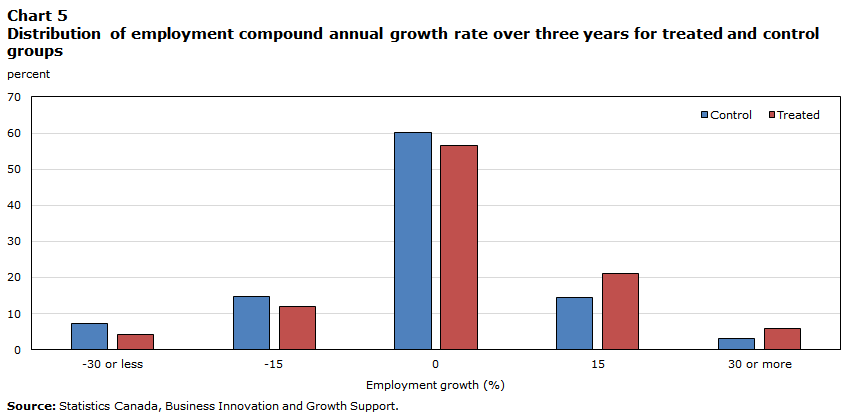
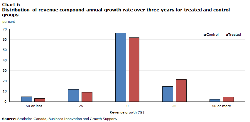
Charts 5 and 6, respectively, compare the distribution of employment and revenue growth of beneficiary and non-beneficiary enterprises, three years after receiving support. Beneficiary enterprises had more positive employment and revenue growth than non-beneficiary enterprises.
Data table for Chart 5
| Employment growth (%) (Midpoint bin) |
Control | Treated |
|---|---|---|
| percent | ||
| -30 or less | 7.3475 | 4.3389 |
| -15 | 14.6746 | 11.9116 |
| 0 | 60.2538 | 56.6312 |
| 15 | 14.5722 | 21.1420 |
| 30 or more | 3.1519 | 5.9763 |
| Source: Statistics Canada, Business Innovation and Growth Support. | ||
Data table for Chart 6
| Revenue growth (%) (Midpoint bin) |
Control | Treated |
|---|---|---|
| percent | ||
| -50 or less | 4.6869 | 3.2133 |
| -25 | 11.9730 | 9.1486 |
| 0 | 66.1891 | 61.8502 |
| 25 | 14.7974 | 21.3876 |
| 50 or more | 2.3537 | 4.4003 |
| Source: Statistics Canada, Business Innovation and Growth Support. | ||
Discussion
In general, the findings align with other studies: Belleau-Arsenault (2017) showed that government financial assistance had a positive impact on employment growth of enterprises in the Bas-Saint-Laurent region between 2006 and 2015. Huang and Rivard (2019) found a positive effect of the Canada Small Business Financing Program on revenue and employment growth of beneficiary enterprises of 6 and 3 percentage points respectively between 2014 and 2016 compared to control group. In Europe between 2005 and 2012, Asdrubali et al. (2015) found that a support program for a small- and medium-sized enterprises had a positive impact on the employment of beneficiary enterprises. Finally, Vanino et al. (2019) observed the positive effect on employment and sales growth of innovation and R&D grants in the United Kingdom between 2004 and 2016.
It would be interesting in a future study to compare the match obtained with the results based on different matching methods. Although the propensity score method used in this study was validated, it could also be combined with a difference in difference approach. If the outcome follows the same trend in the treated and control group over several years prior to support, a difference in difference approach can compare the outcome before and after support in each group and then compare the observed difference in the treated group with the observed difference in the control group. On the one hand, the propensity score controlled the selection bias caused by observed variables and, on the other hand, the difference in difference approach can control selection bias caused by unobserved variables (Lecocq et al., 2014).
Generalized propensity score methods for continuous treatment (e.g. Wu et al., 2020) were developed in past decades. Although there are few applications in the field of program evaluation. Such generalized propensity score methods for continuous treatment could be used in future impact assessments by considering the value of support as treatment.
New explanatory variables could be incorporated into the model to limit selection bias. For instance, variables related to eligibility criteria for program streams in this study, a variable indicating whether or not an enterprise is innovating, a variable showing an enterprise’s employment two years before receiving support or a variable indicating whether or not an enterprise uses debt as financial leverage.
The impact of business innovation and growth support (BIGS) could be assessed on additional outcomes such as productivity or R&D expenditures and over a longer period in order to determine if the support had an impact on business investments and innovation, for instance.
While this analysis examines the impact of business innovation and growth support independently of federal program streams, similar analyses by program stream would be relevant, including a part of performance evaluation.
The analysis showed that a majority of beneficiary enterprises received advisory services for which there is no support value. It would be interesting in a future study to assess the impact of advisory services on enterprise performance. Such an analysis would examine whether advisory services improve enterprise performance in the same way as other types of support, such as grants, despite the fact that they do not provide financial support to enterprises.
Conclusion
The purpose of this analysis was to answer the following question: Did the support from federal program streams for business innovation and growth have an impact on the performance of beneficiary enterprises between 2007 and 2017?
Using the business innovation and growth support data linked to Statistics Canada’s Linkable File Environment and a propensity score matching method, the results showed that BIGS program streams appear to have had a positive and significant effect on employment and revenue growth of beneficiary enterprises.
Appendix
| Type of support | Description |
|---|---|
| Advisory service | External service where data, information or advice is conveyed to an enterprise. For the purpose of BIGS program streams, advisory services are not cost-recovered. Examples of advisory services: increasing awareness of Government of Canada policies, programs and services, or information made available through an online database, publication or call centre. |
| Non-repayable contribution | A form of contribution that is exempt from repayment for such purposes that are specified in the Directive on Transfer Payments. |
| Consortium member | An enterprise that is not the recipient of support but is a joint member of a project with at least one recipient of support. Support for this business is expected to have an economic impact. |
| Unconditionally repayable contribution | A transfer payment that is repayable in part or in full for which no condition of repayment is specified in a funding agreement. |
| Grant | A transfer payment subject to pre-established eligibility and other entitlement criteria. A grant is not subject to being accounted for by a recipient nor normally subject to audit by the department or agency. The recipient may be required to report on results achieved. |
| Service fully cost-recovered | A service that is provided to the client, where the cost of the service is assumed in full by the client. |
| Conditionally repayable contribution | Contribution where repayment obligations are triggered by predetermined events or circumstances, and where repayment in full may not be required. |
| Service partially cost-recovered | A service that is provided to the client, where the cost of the service is partially but not completely assumed by the client. |
| Targeted procurement | Use of federal procurement as an instrument for business innovation or support programming to achieve economic or innovation policy objectives. |
| Sources: Glossary for Business Innovation and Growth Support (BIGS) Programs (September 2019) and Business Program Administrative Data Specification (November 2018), Treasury Board of Canada Secretariat | |
| Subsector | Beneficiary enterprises (N=12,527) | Value of support to enterprises | ||
|---|---|---|---|---|
| number | proportion (percent) | thousands of $ | proportion (percent) | |
| Food manufacturing | 1,458 | 11.6 | 297,543 | 6.3 |
| Beverage and tobacco product manufacturing | 416 | 3.3 | 36,475 | 0.8 |
| Wood product manufacturing | 659 | 5.3 | 163,059 | 3.5 |
| Paper manufacturing | 133 | 1.1 | 118,877 | 2.5 |
| Chemical manufacturing | 894 | 7.1 | 277,227 | 5.9 |
| Plastics and rubber products manufacturing | 661 | 5.3 | 94,090 | 2.0 |
| Fabricated metal product manufacturing | 1,424 | 11.4 | 156,123 | 3.3 |
| Machinery manufacturing | 1,781 | 14.2 | 893,091 | 19.0 |
| Computer and electronic product manufacturing | 1,191 | 9.5 | 445,885 | 9.5 |
| Electrical equipment, appliance, and component manufacturing | 569 | 4.5 | 158,013 | 3.4 |
| Transportation equipment manufacturing | 767 | 6.1 | 1,612,365 | 34.3 |
| Furniture and related product manufacturing | 441 | 3.5 | 50,274 | 1.1 |
| Miscellaneous manufacturing | 1,353 | 10.8 | 195,441 | 4.2 |
| Other manufacturing subsectors | 1,194 | 9.5 | 208,812 | 4.4 |
| Source: Statistics Canada, Business Innovation and Growth Support. | ||||
| Program stream | Beneficiary enterprises (N=12,527) | Value of support to enterprises | ||
|---|---|---|---|---|
| number | proportion (percent) | thousands of $ | proportion (percent) | |
| AgriInnovation Program | 33 | 0.3 | 87,246 | 1.9 |
| Commercialization and Export | 267 | 2.1 | 37,938 | 0.8 |
| Productivity and Expansion | 901 | 7.2 | 395,418 | 8.4 |
| Applied Research and Development Grants | 486 | 3.9 | Note ...: not applicable | 0.0 |
| Collaborative Research and Development Grants | 675 | 5.4 | Note ...: not applicable | 0.0 |
| Engage Grants | 1,376 | 11.0 | Note ...: not applicable | 0.0 |
| Innovation Enhancement Grants | 318 | 2.5 | Note ...: not applicable | 0.0 |
| Industrial Research Chairs | 205 | 1.6 | Note ...: not applicable | 0.0 |
| Strategic Partnership Grants for Projects | 346 | 2.8 | Note ...: not applicable | 0.0 |
| Industrial Research Assistance Program | 8,070 | 64.4 | 519,572 | 11.0 |
| Aerospace | 51 | 0.4 | 55,551 | 1.2 |
| ecoENERGY for Renewable Power | 9 | 0.1 | 85,234 | 1.8 |
| Investments in Forest Industry Transformation | 19 | 0.2 | 112,126 | 2.4 |
| CanExport | 278 | 2.2 | 5,192 | 0.1 |
| Trade Commissioner Service | 4,968 | 39.7 | Note ...: not applicable | 0.0 |
| Automotive Innovation Fund | 5 | 0.0 | 391,857 | 8.3 |
| Strategic Aerospace and Defence Initiative | 21 | 0.2 | 1,322,606 | 28.1 |
| Technology Partnerships Canada | 37 | 0.3 | 486,577 | 10.3 |
| Sustainable Development Technology Canada | 87 | 0.7 | 279,975 | 5.9 |
| Advanced Manufacturing Fund | 7 | 0.1 | 81,993 | 1.7 |
| Investing in Business Growth and Productivity | 388 | 3.1 | 102,913 | 2.2 |
| Mitacs Inc. | 354 | 2.8 | Note ...: not applicable | 0.0 |
| Automotive and Surface Transportation | 179 | 1.4 | 33,506 | 0.7 |
| Other program streams | 2,357 | 18.8 | 709,572 | 15.1 |
|
... not applicable Source: Statistics Canada, Business Innovation and Growth Support. |
||||
| Year | Treated enterprises | Value of support to treated enterprises | Potential control enterprises | Pairs |
|---|---|---|---|---|
| number | thousands of $ | number | ||
| 2007 | 978 | 184,272 | 41,933 | 929 |
| 2008 | 704 | 34,379 | 41,224 | 689 |
| 2009 | 609 | 31,216 | 40,361 | 590 |
| 2010 | 460 | 27,596 | 39,459 | 447 |
| 2011 | 391 | 19,375 | 37,816 | 376 |
| 2012 | 698 | 24,440 | 36,377 | 672 |
| 2013 | 1,393 | 24,550 | 35,380 | 1,354 |
| 2014 | 958 | 22,973 | 37,940 | 919 |
| 2015 | 926 | 13,029 | 37,673 | 890 |
| 2016 | 802 | 35,727 | 37,204 | 776 |
| 2017 | 610 | 27,213 | 36,855 | 571 |
| Source: Statistics Canada, Business Innovation and Growth Support. | ||||
References
Asdrubali, P. & Signore, S. (2015). The Economic Impact of EU Guarantees on Credit to SMEs – Evidence from CESEE Countries. EIF Working Paper Series 2015/29, European Investment Fund (EIF). http://ec.europa.eu/economy_finance/publications/
Biagi, F., Bondonio, D. & Martini, A. (2015). Counterfactual Impact Evaluation of Enterprise Support Programmes. Evidence from Decade of Subsidies to Italian Firm, 55th Congress of the European Regional Science Association: “World Renaissance: Changing roles for people and places”, 25-28 August 2015, Lisbon, Portugal, European Regional Science Association (ERSA), Louvain-la-Neuve. http://hdl.handle.net/10419/124844
Belleau-Arsenault, C. (2017). Les impacts des aides financières gouvernementales sur la performance des entreprises en région : une approche par appariement spatial. Université Laval, Québec.
Bérubé, C. & Therrien, P. (2016). Direct and Indirect Support to Business R&D. Internal. Ottawa: Economic Research and Policy Analysis Directorate, Innovation, Science and Economic Development Canada.
Burden, A. et al. (2017). An evaluation of exact matching and propensity score methods as applied in a comparative effectiveness study of inhaled corticosteroids in asthma. Pragmatic and Observational Research. https://www.ncbi.nlm.nih.gov/pubmed/28356782
Caliendo, M. & Kopeinig, S. (2005). Some Practical Guidance for the Implementation of Propensity Score Matching. Institute for the Study of Labor, IZA DP No. 1588.
Huang, L. & Rivard, P. (2019). Canada Small Business Financing Program: Economic Impact Analysis. Ottawa: Innovation, Science and Economic Development Canada. July 2019.
Kelly, R. & Kim, H. (2013). Venture Capital as a Catalyst for High Growth. Ottawa: Industry Canada. https://www.ic.gc.ca/eic/site/eas-aes.nsf/eng/h_ra02218.html#p3.2
Lecocq, A., Ammi, M. & Bellarbre, É. (2014). Le score de propension : un guide méthodologique pour les recherches expérimentales et quasi expérimentales en éducation. Mesure et évaluation en éducation, 37 (2), 69–100. https://doi.org/10.7202/1035914ar
Rosenbaum, P. & Rubin, D. (1983). The central role of the propensity score in observational studies for casual effects, Biometrika, 70 (1), 41-55.
SAS Institute Inc. (2016). SAS/STAT® 14.2 User’s Guide. Cary, NC: SAS Institute Inc.
Statistics Canada, Data Integration Infrastructure Division (2020). Business register data, https://www.statcan.gc.ca/eng/statistical-programs/document/1105_D16_V3#a5
Statistics Canada. (2018). North American Industry Classification System (NAICS) Canada 2017 Version 3.0. Statistics Canada Catalog no. 12-501-X. Ottawa: Statistics Canada.
Statistics Canada. (2020). Table 33-10-0221-01. Enterprises (ultimate beneficiary) with business innovation and growth support by industry and year. https://www150.statcan.gc.ca/t1/tbl1/fr/tv.action?pid=3310022101
Stuart, E. A. (2010). Matching methods for causal inference: A review and a look forward. Statistical science: a review journal of the Institute of Mathematical Statistics, 25(1), 1-21. https://doi.org/10.1214/09-STS313
Vanino, E., Roper, S. & Becker, B. (2019). Knowledge to money: Assessing the business performance effects of publicly-funded R&D grants, Research Policy 48, 1714-1737.
Wu, X., Mealli, F., Kioumourtzoglou, M., Dominici, F. & Braun, D. (2020). Matching on Generalized Propensity Score with Continuous Exposures, arXiv :1812.06575, https://arxiv.org/pdf/1812.06575.pdf
Notes
- Date modified: