
Bayesian hierarchical weighting adjustment and survey inference
Section 5. Application to longitudinal study of wellbeing
With the background introduced in Section 2, we apply the prediction and weighting inference to the NYC Longitudinal Study of Wellbeing. We match the LSW to the adult population via the ACS. We would like to conduct finite population and domain inference and generate weights allowing for general analysis use. The outcome of interest is the self-reported score of life satisfaction on a 1 10 scale. We model the outcome as normally distributed, which is not quite correct given that the responses are discrete, but should be fine in practice for the goal of estimating averages. We first include the same eight variables to construct the poststratification cells and use the same estimation model as those in Section 4.2 under the structured prior setting. The posterior inference shows that the variables sex, cldx, eldx, and psx are not predictive, and neither are the related high-order interactions. The scale estimates of such terms have posterior median values close to 0 and several large values as long tails. The posterior samples of scales for several high-order interactions among the remaining four variables concentrate around 0, showing these quantities are not predictive. Another complexity is that, for the sample cells of the LSW, the corresponding population cells are not available in the ACS data. This could happen because the sampling frame is not the ACS survey. The population information is unknown for such cells, and untestable assumptions have to be made. The model fitting improves after variable selection when we check the prediction errors for cell estimates.
Hence, we use four variables after selection, age, eth, edu and pov, which constructs 500 poststratification cells. The 2,002 units in the LSW spread out in 359 cells. The largest sample cell has 86 units, while 92 cells have only one unit. The covariates in the model (3.4) for cell estimates include the main effects of the four variables, five two-way interactions (age * eth, age * edu, eth * edu, age * inc and eth * inc), and two three-way interactions (age * eth * edu and age * eth * inc). We implement the fully Bayesian inference with the structured prior distributions. We are interested in estimating the average score of life satisfaction for overall and several subgroups of NYC adults and construct weights for general analysis purposes using the LSW.
The posterior median of the unit scale inside cells is 1.93 with 95% credible interval [1.87, 1.99]. The posterior median of the group scale is 0.79 with 95% credible interval [0.65, 1.02]. These lead to moderately large shrinkage effects between 0.11 and 0.90 with mean 0.30 across cells. The moderate shrinkage effect makes sense based on the four variables and up to three-way interactions being included. The posterior mean values of the model-based weights are presented in the left plot of Figure 5.1. We can generate the raking weights after adjustment for the marginal distributions of the four variables and poststratification weights based on the ACS data. The population information is obtained after applying the ACS personal weights.
Comparing with the classical weights, our model-based weights have smaller variability with standard deviation 0.32 and the ratio of the maximum and minimum value 3.87, and these values are much smaller than those for the raking and poststratification weights, as shown in Table 5.1. The right plot in Figure 5.1 shows the distribution of the lift satisfaction score after weighting. The model-based weighted distributions and classically weighted distributions are similar as expected, which is consistent with the results in Section 4.2. The weighting process adjusts for the sample distribution by upweighting the high scores and downweighting the low scores. The LSW oversamples poor residents who tend not be satisfied with life, and the weighting adjustment balances the discrepancy.
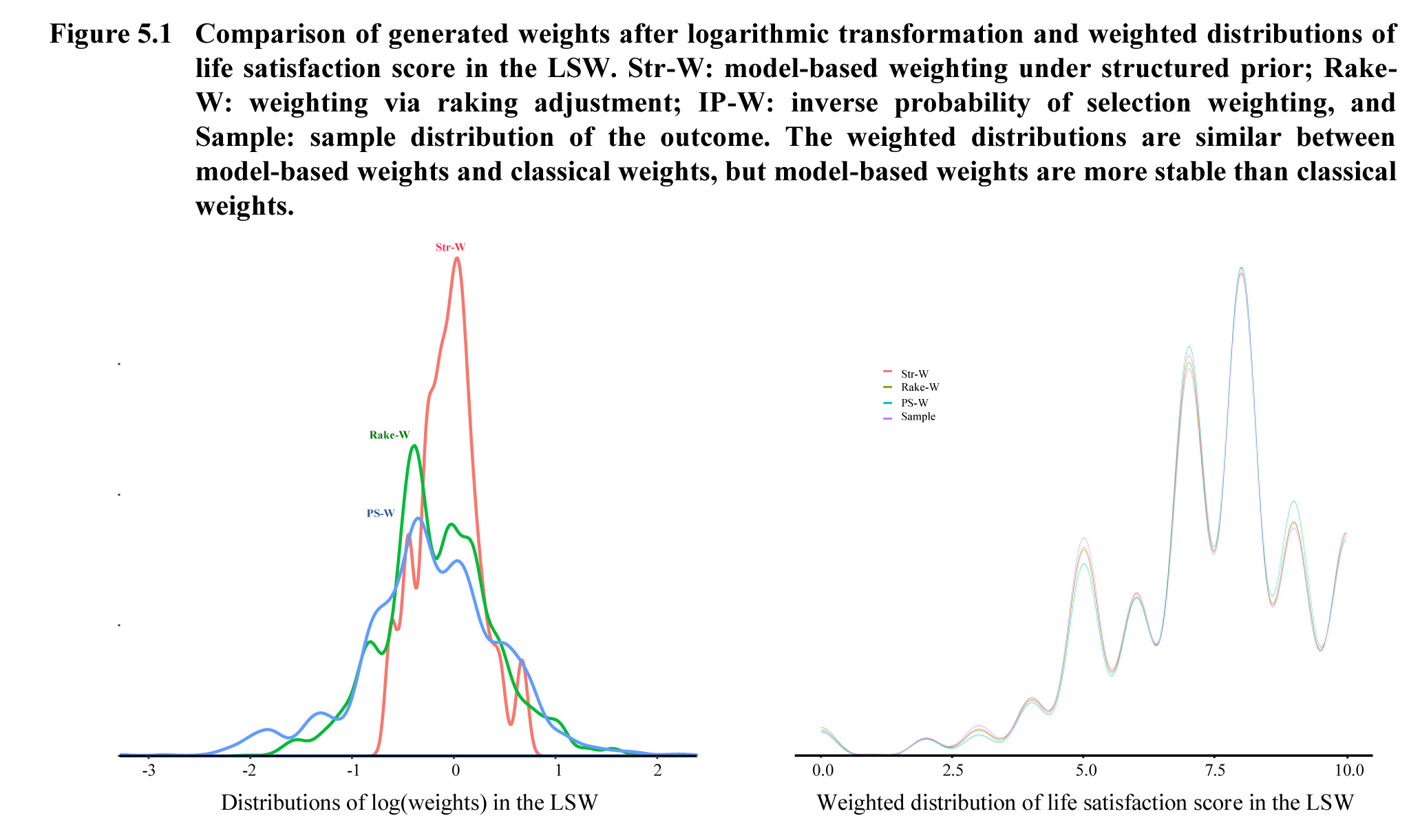
Description for Figure 5.1
Figure presenting two graphs. The first one shows the distributions of log (weights) in the LSW. There are three curves: Str-W, Rake-W and PS-W. The x-axis ranges from -3 to 2. Rake-W and PS-W are close. Str-W is narrower and reaches a higher peak around 0. The second graph is the weighted distribution of life satisfaction score in the LSW. There are four curves: Str-W, Rake-W, PS-W and Sample. The x-axis ranges from 0.0 to 10.0. The weighted distributions are similar between model-based weights and classical weights, but model-based weights are more stable than classical weights.
Table 5.1 and Figure 5.2 present the finite population and domain inference. The average score of life satisfaction for NYC adults is 7.24 with standard error 0.05, predicted by the structural model. The estimate is similar to that under model-based weighting and raking inferences, but lower than the poststratification weighting inference. However, the difference is not significant. For example, the structural model predicts the average score of life satisfaction for middle-aged, college-educated whites with income more than three times the poverty level as 7.40 with standard error 0.10, higher than that under weighting inferences. Nevertheless, the predicted scores for the elder with relatively low income (7.37 with SE 0.15) and low-income black New Yorkers (7.01 with SE 0.18) are lower than those under weighting inferences. The discrepancy could be explained by the nonrepresentativeness of the LSW and the deep interactions included by the model. The subgroup of individuals who are middle-aged, college-educated whites may be undercovered in the LSW − as empty poststratification cells occurring − with overcoverage among elderly poor blacks. Weighting the collected samples cannot infer or extrapolate inference on those who are not present in the survey. Though the differences are not significant, inferences conditioning on the collected samples cannot recover the truth, especially for the empty cell estimates. Figure 5.2 shows the model-based prediction yields a higher score for young, highly educated and Hispanic NYC adults, but a lower score for those with poverty gap 50%, comparing with the weighted inference.
| Str-P | Str-W | Rake-W | PS-W | |
|---|---|---|---|---|
| SD of weights / mean of weights | This is an empty cell | 0.32 | 0.66 | 0.80 |
| Max weight / min weight | This is an empty cell | 3.87 | 81.28 | 274.65 |
| Overall average for NYC adults ( 2,002) | ||||
| Est | 7.24 | 7.23 | 7.24 | 7.30 |
| SE | 0.05 | 0.05 | 0.05 | 0.06 |
| Average for middle-aged, college-educated whites with poverty gap 300% ( ) | ||||
| Est | 7.40 | 7.34 | 7.34 | 7.34 |
| SE | 0.10 | 0.11 | 0.11 | 0.11 |
| Average for elders with poverty gap 200% ( ) | ||||
| Est | 7.37 | 7.52 | 7.49 | 7.53 |
| SE | 0.15 | 0.18 | 0.19 | 0.22 |
| Average for blacks with poverty gap 50% ( ) | ||||
| Est | 7.01 | 7.16 | 7.30 | 7.16 |
| SE | 0.18 | 0.26 | 0.28 | 0.29 |
The SEs are similar for the overall mean estimation between predictions and various weighting inferences because of the large sample size. For domain estimation, the model-based prediction and weighting are more efficient than that with raking and poststratification weighting, and the model-based prediction has the smallest standard error. The efficiency gains of model-based prediction and weighting are further demonstrated by domain mean estimation for life satisfaction scores across the marginal levels of four variables, shown in Figure 5.2. The model-based prediction and weighting particularly improve small domain estimation and increase the efficiency.
Survey practitioners often compare the weighted distribution of socio-demographics with the population distribution to check the weighting. While weighting diagnostics need further research and management, we follow this routine to compare the model-based and classical weights. We calculate the Euclidean distances between the weighted distributions and the population distribution for the main effects and high-order interactions among the four variables in the LSW, shown in Table B.6 in Appendix B. The weighted distributions are generally close to the true distributions. Raking focuses on adjusting for the marginal distributions of calibration variables but distorts the joint distributions, where the dependency structure is determined only by the sample without calibration. The poststratification weighting adjusts for the joint distribution, but empty cells in the sample present from the exact matching. The unbalanced cell structure yields unstable inference. The model-based weighting smooths the poststratification weightings and outperforms raking to match the distributions of three-way and four-way interaction terms. Practitioners often rely upon the marginal distributions to evaluate weighting performances, thus in favor of raking. However, raking yields high variable and potentially biased inferences, shown in the Section 4, even in the cases when raking adjustment is correct. Modification of model-based weighting to satisfy such desire on matching marginal distributions will be a future extension to incorporate constraints.
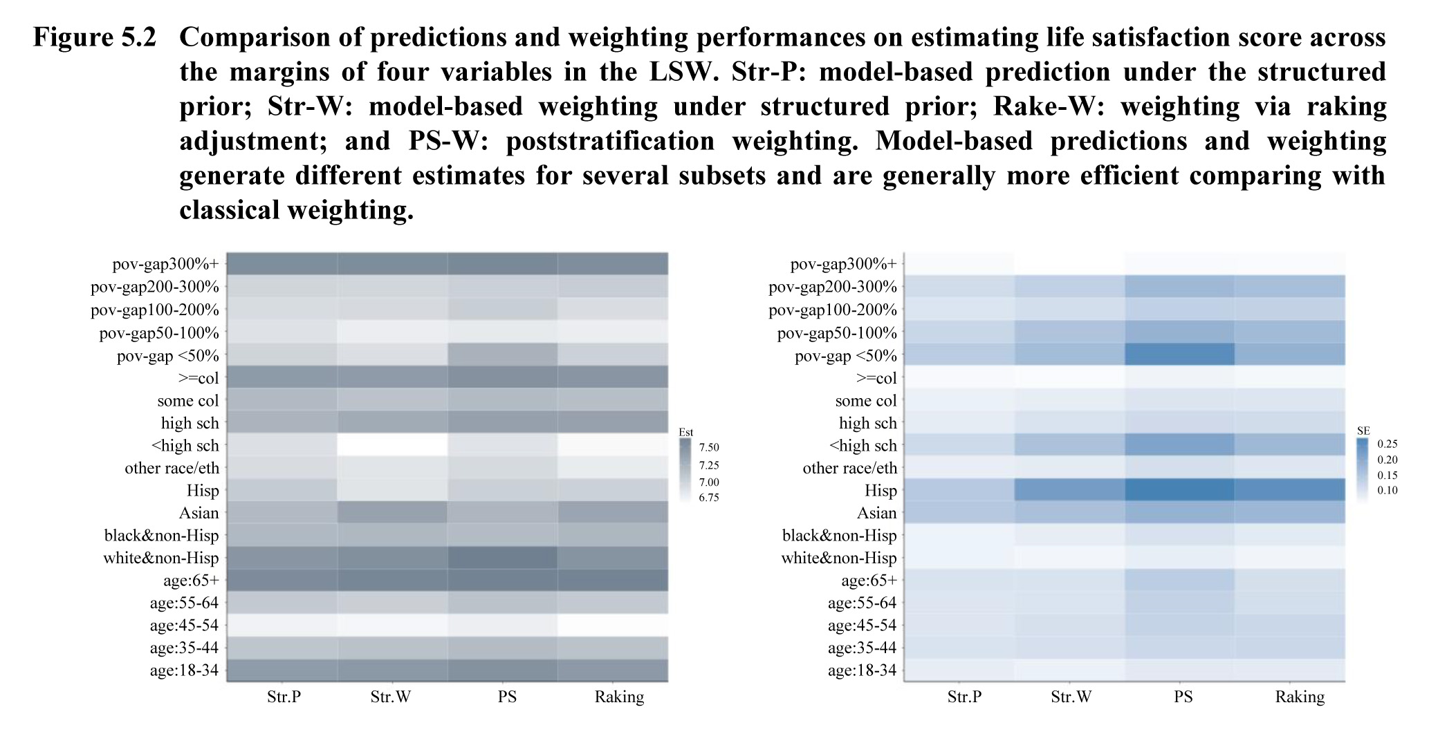
Description for Figure 5.2
Comparison of predictions and weighting performances on estimating life satisfaction score across the margins of four variables in the LSW. Two graphs are presented: the estimate (from 6.75 to 7.50) and the SE (from 0.10 to 0.25). For all graphs, the y-axis denotes different groups: poverty gap (<50%, 50-100%, 100-200%, 200-300%, 300%+), education breakdown (less than high school, high school, some college, college or more), race breakdown (White & non-Hispanic, Black & non-Hispanic, Asian, Hispanic, other race/ethnicity) and age breakdown (18-34, 35-44, 45-54, 55-64, 65+). The x-axis shows the methods: Str-P, Str-W, Rake-W and PS-W. Model-based predictions and weighting generate different estimates for several subsets and are generally more efficient comparing with classical weighting.
- Date modified: