Robust variance estimators for generalized regression estimators in cluster samples
Section 3. Simulation
We performed a series of simulation studies to test the performance
of the new variance estimators in different populations. In each simulated
sample, we computed the quantities listed in Table 3.1. To evaluate the
variance estimators, we calculated the average of the variance estimates,
compared those averages to the empirical mean square error, and computed
coverage probabilities of confidence intervals based on the different variance
estimates. Table 3.2 summarizes the sample designs for the 18 simulation
studies. The column called Label gives the headings used in later tables. The
sample designs are used in three populations described below.
Table 3.1
Statistics of interest for clustered GREG variance simulation
Table summary
This table displays the results of Statistics of interest for clustered GREG variance simulation. The information is grouped by Statistic (appearing as row headers), Description (appearing as column headers).
| Statistic |
Description |
|
Estimated total from the Horvitz-Thompson Estimator |
|
Estimated total from the GREG |
|
Empirical variance |
|
Design-based variance estimator that assumes Poisson sampling at both stages from Särndal et al. (1992) in (2.3) |
|
With-replacement variance estimator in (2.4) |
|
Jackknife linearization variance estimator from Yung and Rao (1996) in (2.5) |
|
Sandwich estimator in (2.8) |
|
First hat-matrix adjusted sandwich estimator in (2.11) |
|
Jackknife variance estimator in (2.6) |
|
First approximation to the jackknife variance estimator in (2.13) |
|
Second approximation to the jackknife variance estimator in (2.14) |
|
Sandwich estimator with a finite population adjustment |
|
First hat-matrix adjusted sandwich estimator with a finite population correction |
|
Jackknife variance estimator with a finite population correction |
|
First approximation to jackknife with a finite population correction |
|
Second approximation to jackknife with a finite population adjustment |
3.1 Data
We
conducted simulations on three populations to assess the design-based
performance of the variance estimators under a variety of situations. In the
first population, we investigated the performance of the variance estimators
when the first-stage sampling fraction was large and the sample size was
moderate. The focus of the second simulation study was on the performance of
the variance estimators under a relatively messy dataset and a small
first-stage sample size. The final simulation study shows the performance of
the variance estimators in large samples.
Table 3.2
Simulation designs for three populations
Table summary
This table displays the results of Simulation designs for three populations Label, Population, First stage sample, (équation), Second stage sample and No. of samples (appearing as column headers).
|
Label |
Population |
First stage sample |
|
Second stage sample |
No. of samples |
| 1 |
srs fixed |
Third Grade |
srswor |
25 |
|
1,000 |
| 2 |
srs fixed |
Third Grade |
srswor |
50 |
|
1,000 |
| 3 |
srs epsem |
Third Grade |
srswor |
25 |
|
1,000 |
| 4 |
srs epsem |
Third Grade |
srswor |
50 |
|
1,000 |
| 5 |
pps epsem |
Third Grade |
ppswor |
25 |
|
1,000 |
| 6 |
pps epsem |
Third Grade |
ppswor |
50 |
|
1,000 |
| 7 |
srs fixed |
ACS |
srswor |
3 |
|
5,000 |
| 8 |
srs fixed |
ACS |
srswor |
15 |
|
5,000 |
| 9 |
srs epsem |
ACS |
srswor |
3 |
|
5,000 |
| 10 |
srs epsem |
ACS |
srswor |
15 |
|
5,000 |
| 11 |
pps epsem |
ACS |
ppswor |
3 |
|
5,000 |
| 12 |
pps epsem |
ACS |
ppswor |
15 |
|
5,000 |
| 13 |
srs fixed |
Simulated |
srswor |
300 |
|
1,000 |
| 14 |
srs fixed |
Simulated |
srswor |
1,500 |
|
100 |
| 15 |
srs epsem |
Simulated |
srswor |
300 |
|
1,000 |
| 16 |
srs epsem |
Simulated |
srswor |
1,500 |
|
100 |
| 17 |
pps epsem |
Simulated |
ppswor |
300 |
|
1,000 |
| 18 |
pps epsem |
Simulated |
ppswor |
1,500 |
|
100 |
3.1.1 Third grade population
The
first simulation study used the Third Grade population from Appendix B.6 of Valliant
et al. (2000). This dataset contained the mathematics achievement scores
for 2,427 third graders in 135 schools. The relatively small number of schools
in this population and the fairly constant number of students in each school
made it ideal for studying samples with large sampling fractions.
We
used GREG to estimate the average mathematics achievement score for third
graders. Altogether, we selected 1,000 samples in each of six sample designs
listed in Table 3.2. In the first sample design, we selected 1,000 simple
random samples without replacement (srswor)
of 25 schools. Within each sampled school, we selected exactly five students
via srswor. Because the number
of students in each school varied from school to school, this sample design
resulted in different unconditional probabilities of selection, but a fixed
sample size of 125 students. The second sample design was similar to the first,
except we selected 50 schools. Selecting 50 of the 135 schools resulted in a
large first-stage sampling fraction of 0.37, necessitating a finite population
correction factor. Both the samples of
25 and 50 might be considered to be of
“moderate” size.
In
the third sample design, we selected 1,000 simple random samples of 25 schools
without replacement. Within each sampled school, we selected students at a
constant rate of
yielding 1,000 samples with random sizes
centered around 125 students. The result of this design was that each student
had the same unconditional probability of selection. The fourth sample design
was similar to the third, except we selected 50 schools. The sample sizes were
also random under this design, with an average of 250 students. Since the third
and fourth sample designs resulted in every unit getting the same chance of
selection, these sample designs are labeled srs epsem (equal
probability selection mechanism) in subsequent tables.
In
the fifth design, we selected 1,000 samples of 25 schools with probabilities
proportional to the number of students in each school. Within each sampled
school, we selected exactly five students, yielding 1,000 samples with exactly
125 students each. The sixth sample design was similar to the fifth, except we
selected 50 schools. We selected 1,000 samples of size 250 students using this
design. The fifth and sixth designs are epsem.
Like the second and fourth sample designs, this sample design also had a large
sampling fraction and warranted the need for a finite population correction
factor to adjust the variance estimators.
From
each sample, we estimated the average achievement scores for the finite
population using a GREG estimator and assuming that the number of students in
the population was known. The assisting model was meant to replicate the
clustered linear regression model in Section 9.6 of Valliant et al.
(2000). The eleven explanatory variables used to model each student’s math
achievement score were: an intercept, sex (male or female), ethnicity
(White/Asian, Black, Native American/Other, or Hispanic), language spoken at
home is the same as the test (Always, Sometimes/Never), type of community
(Outskirts of a town or city, Village/City), and school enrollment. The total
mathematics achievement estimated with the GREG estimator was divided by the
number of students in the population, 2,427, to get the average achievement
score. The average achievement score for the population was 477.7. For the full
population, the R-squared for the student-level linear model was 0.9735,
indicating a very strong linear relationship.
3.1.2 American Community Survey population
The
second simulation study used Census 2000 Summary File 3 data and American
Community Survey (ACS) 2005 - 2009 Summary File data. The goal was to estimate
the total number of housing units in the U.S. state of Alabama as reported in
the ACS Summary File. Block group counts from Census 2000 were used as
covariates in the assisting model.
To
create the population, first all block group data were extracted from the ACS
Summary File and the Census 2000 Summary File 3. Then, the two files were
merged at the block group level. Block groups with 1,000 or more housing units
in Census 2000 were removed because such large block groups had different
characteristics than the majority of blocks. In many sampling designs such
large units would be placed in a separate, certainty stratum and not contribute
to the variance of estimates. Also, block groups with extreme growth in the total
number of housing units were also removed. Specifically block groups that had
gained more than 10 units over twice the 2000 census count were removed.
Clusters
were defined as counties and block groups were treated as units. Treating block
group as a unit is motivated by the common task of selecting a sample of
blocks, listing them, and then using the listings to estimate the total number
of housing units in the finite population.
Clusters
with fewer than 10 block groups or more than 120 block groups in them were
removed from the frame of clusters. Overall, there were 61 clusters (counties)
containing a total of 2,051 block groups and 1,109,499 housing units in the
edited dataset. Altogether, six counties and 1,278 block groups containing
1,030,471 housing units were removed from the Alabama file.
Figure 3.1
shows two scatterplots. The first plot shows the total number of housing units
in the block group as reported on the ACS summary file as a function of the
2000 Census housing unit count. Each point represents one of the 2,051 block
groups in the finite population. The diagonal line is a nonparametric smoother,
indicating a strong relationship between the two variables. The plot also shows
some evidence of heteroscedasticity because the points appear to fan out as the
2000 census count increases. The second plot shows the residuals obtained by
regressing the 2000 census housing unit count on the ACS housing unit count
using ordinary least squares (OLS) plotted versus the ACS housing unit count.
As the number of housing units reported on the ACS file increases, the model
predictions appear to seriously underestimate the true number of housing units.
This suggests some degree of nonlinearity in the mean function. In addition,
there is noticeable heteroscedasticity in variance.
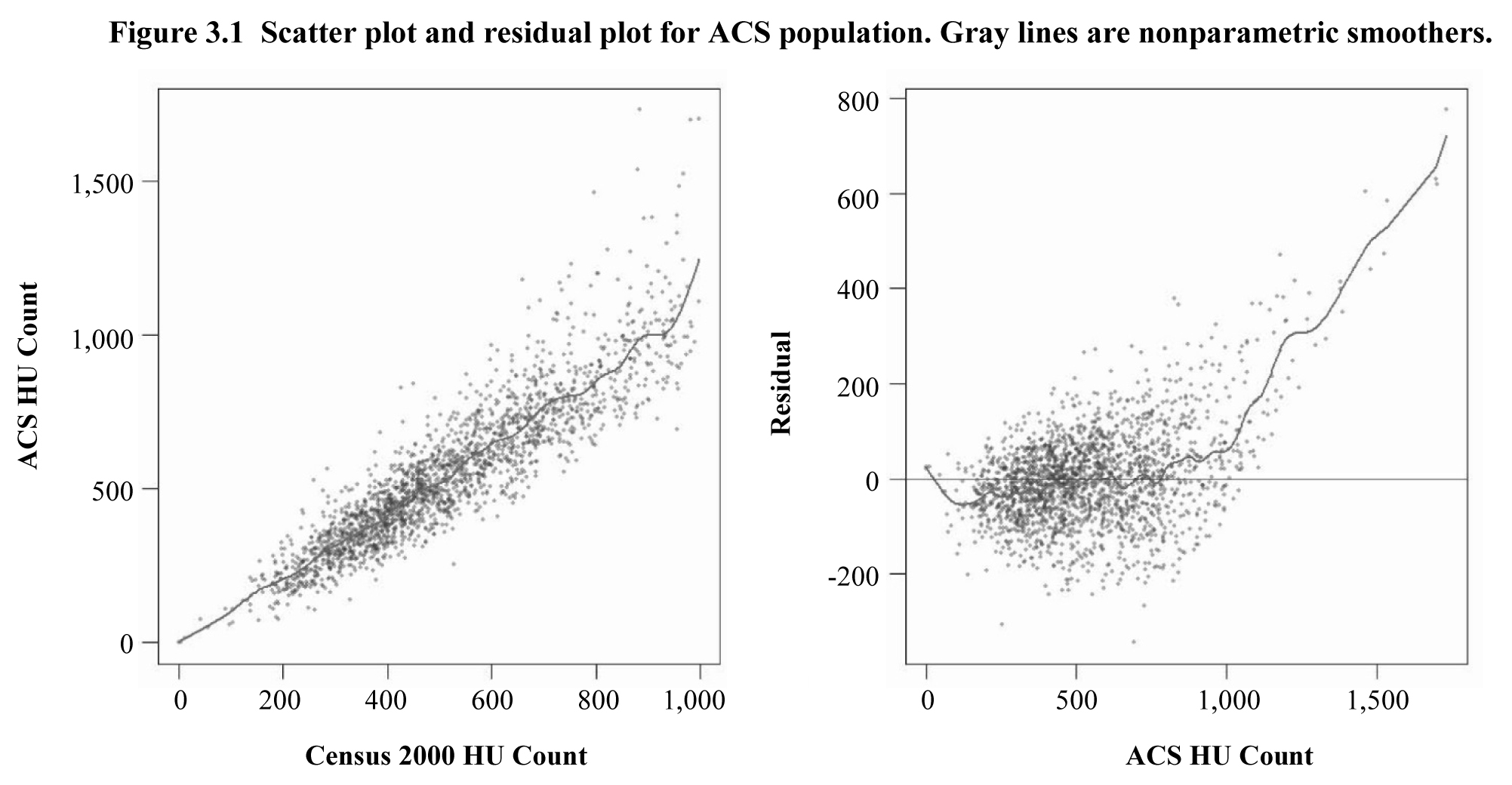
Description for Figure 3.1
Figure showing two scatter plots for the ACS population. The first graph illustrates the ACS HU count on then y-axis, going from 0 to 1,500, versus the Census 200 HU count on the x-axis, going from 0 to 1,000. A line representing a nonparametric smoother goes through the scatter plot and shows a strong relationship between the two variables. There is evidence of heteroscedasticity because the points appear to fan out as the 2000 census count increases. The second graph presents the residual on the y-axis, going from -200 to 800, versus the ACS HU count on the x-axis, going from 0 to 1,500. A line representing a nonparametric smoother goes through the scatter plot. As the number of housing units reported on the ACS file increases, the model predictions appear to seriously underestimate the true number of housing units. This suggests some degree of nonlinearity in the mean function. In addition, there is noticeable heteroscedasticity in variance.
As in the first simulation study, we tested six
different sample designs. We selected 5,000 samples in each of six different
selection mechanisms listed in Table 3.2. In the first sample design, we
selected 5,000 simple random samples of 3 clusters without replacement. In
large national surveys, it is not uncommon to select a small number of primary
sampling units in each stratum. In this case, we treat Alabama as if it were a
single design stratum and its 61 counties as clusters. Three counties within
that stratum were sampled. Within each cluster, we selected nine block groups
using srswor. The second design
was similar with 15 clusters and 9 block groups per cluster. The first two
sample designs resulted in highly variable weights. The other designs (rows
9-12) were parallel to those in rows 3-6 for the Third Grade population. The
sample sizes of
3 and 15 are small so that theoretical, large
sample properties are less likely to hold.
From each sample, we estimated the total number of
housing units in the finite population using a GREG estimator. The assisting
model included an intercept and the Census 2000 count of housing units; the
heteroscedasticity noted above was not accounted for in the GREG. For the full
population, the R-squared was 0.819, again indicating a strong linear
relationship.
3.1.3 Simulated population
A population was created with a large number of clusters
to assess the asymptotic characteristics of the variance estimators. Generated
using a classic linear model, a total of 30,000 clusters were created, each
with a random number of units. The number of units in each cluster was
determined by adding three to a uniform random integer between 0 and 7. This
created clusters ranging in size from 3 to 10 units. Altogether, the population
contained 195,164 units within 30,000 clusters. For each unit, a positive
covariate was created as
where
is a normal random variate with mean of 0 and
standard deviation of 1. A random response was created such that
.
Figure 3.2 shows scatter plots of the relationship between
and
for the finite population.
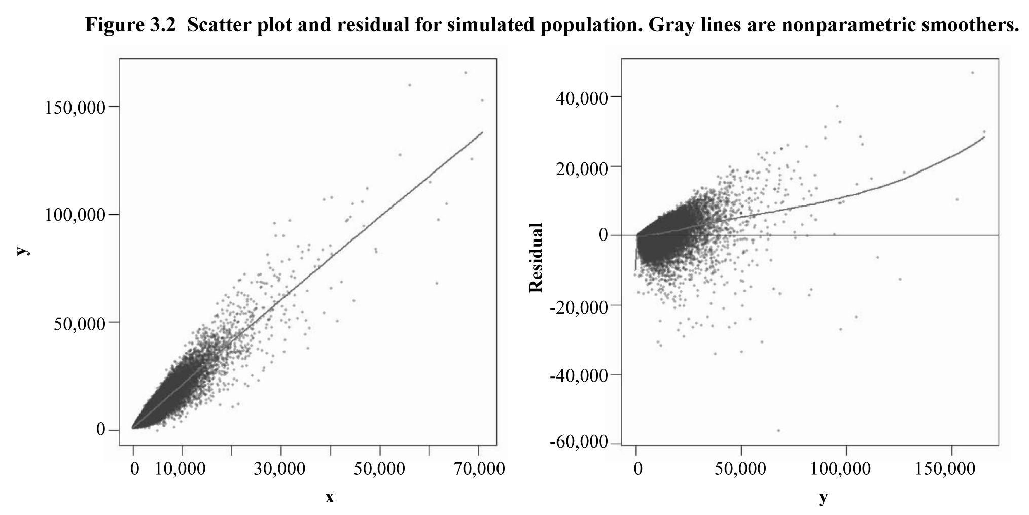
Description for Figure 3.2
Figure showing two scatter plots for a simulated population. For the first graph, the vertical axis presents y, going from 0 to 150,000, versus x, going from 0 to 70,000. A line representing a nonparametric smoother goes through the scatter plot and shows a strong relationship between the two variables. The second graph presents the residual on the y-axis, going from -60,000 to 40,000, versus y, going from 0 to 150,000. A line representing a nonparametric smoother goes through the scatter plot. As y increases, the model predictions appear to underestimate y. In addition, it seems that there is heteroscedasticity in variance.
We
selected samples using the six different probability selection mechanisms
listed in rows 13-18 of Table 3.2. The types of sample designs are
parallel to those used for the Third Grade and ACS populations. In designs 14,
16, and 18, we selected 100 simple random samples of 1,500 clusters without
replacement. We only selected 100 samples due to the excessive amount of
computer time it took to select and process each sample. The sample sizes of
300 and 1,500 are large so that theoretical,
large sample properties should hold.
From
each sample, we estimated the total of the response using a GREG estimator. The
true finite population total was 839,149,969. The assisting model included an
intercept and
with
For the full population, the R-squared was
0.953, indicating a very strong linear relationship. Figure 3.2 shows a
scatter plot of the population as well as a residual plot based on an OLS
regression of
on
for the full population. There is clear
evidence of heteroscedasticity of errors.
3.2 Results
We
explored the bias, variability, and confidence interval coverage of the new and
existing variance estimators. We only show tables for some of the simulations
to conserve space. Table 3.3 shows the means of the
-estimator and the GREG estimator as well as
the ratios of the average values of the variance estimators to the empirical mse’s for all populations and sample
size combinations across all simulations. Both the
-estimator and the GREG estimator are
approximately unbiased; however, the GREG estimator is much more efficient.
Table 3.3
Simulation results for estimates for means and variance estimators for three populations and six sample designs in each population. Values in rows for variance estimators are ratios of mean estimated variance to empirical mse of the GREG. See Table 3.1 for descriptions of the variance estimators
Table summary
This table displays the results of Simulation results for estimates for means and variance estimators for three populations and six sample designs in each population. Values in rows for variance estimators are ratios of mean estimated variance to empirical mse of the GREG. See Table 3.1 for descriptions of the variance estimators. The information is grouped by Estimator (appearing as row headers), srs fixed, srs epsem, pps epsem, Third Grade Population, ACS Population
(numbers in thousands) and Simulated Population
(numbers in millions) , calculated using (équation)25, (équation)50 , (équation)3 , (équation)15 , (équation)300 , (équation)1,500 and (équation)25 units of measure (appearing as column headers).
| Estimator |
srs fixed |
srs epsem |
pps epsem |
| Third Grade Population |
ACS Population
(numbers in thousands) |
Simulated Population
(numbers in millions) |
Third Grade Population |
ACS Population
(numbers in thousands) |
Simulated Population
(numbers in millions) |
Third Grade Population |
ACS Population
(numbers in thousands) |
Simulated Population
(numbers in millions) |
| 25 |
50 |
3 |
15 |
300 |
1,500 |
25 |
50 |
3 |
15 |
300 |
1,500 |
25 |
50 |
3 |
15 |
300 |
1,500 |
| Average |
477.23 |
477.11 |
1,119.13 |
1,108.23 |
838.91 |
838.71 |
476.29 |
476.85 |
1,112.89 |
1,113.89 |
838.13 |
843.13 |
477.31 |
477.75 |
1,111.48 |
1,109.02 |
838.74 |
839.06 |
| mse |
663.12 |
264.75 |
181,329.24 |
27,650.01 |
1,588.43 |
250.20 |
2,013.90 |
981.54 |
201,618.77 |
32,926.98 |
2,303.19 |
563.77 |
142.93 |
53.17 |
15,991.69 |
2,619.32 |
1,218.73 |
253.13 |
| Average |
474.27 |
476.37 |
1,081.68 |
1,103.34 |
838.57 |
839.10 |
476.95 |
477.24 |
1,104.45 |
1,108.45 |
838.81 |
840.01 |
477.50 |
477.85 |
1,106.36 |
1,108.46 |
839.39 |
839.08 |
| mse |
218.96 |
66.66 |
11,220.86 |
921.82 |
156.29 |
23.07 |
114.08 |
50.10 |
2,111.84 |
408.19 |
117.18 |
19.63 |
121.57 |
41.32 |
1,874.39 |
352.65 |
105.64 |
25.24 |
|
0.76 |
0.87 |
2.70 |
0.90 |
0.91 |
1.11 |
0.73 |
0.82 |
0.44 |
0.83 |
0.91 |
1.13 |
0.66 |
0.91 |
0.53 |
0.92 |
1.01 |
0.89 |
|
0.75 |
1.11 |
1.17 |
0.98 |
0.94 |
1.13 |
0.79 |
1.06 |
0.68 |
1.03 |
0.91 |
1.17 |
0.73 |
1.19 |
0.87 |
1.14 |
1.01 |
0.90 |
|
0.88 |
1.16 |
2.18 |
0.91 |
0.91 |
1.13 |
0.85 |
1.10 |
0.65 |
0.99 |
0.92 |
1.15 |
0.78 |
1.24 |
0.79 |
1.11 |
1.02 |
0.90 |
|
0.87 |
1.15 |
2.80 |
1.00 |
0.91 |
1.13 |
0.82 |
1.08 |
0.43 |
0.92 |
0.92 |
1.14 |
0.74 |
1.22 |
0.53 |
1.03 |
1.02 |
0.90 |
|
1.26 |
1.32 |
6.09 |
1.32 |
1.03 |
1.15 |
1.09 |
1.25 |
0.84 |
1.08 |
0.96 |
1.16 |
0.95 |
1.36 |
0.89 |
1.15 |
1.07 |
0.91 |
|
2.22 |
1.54 |
17,191.52 |
1.85 |
1.50 |
1.17 |
1.50 |
1.46 |
2.36 |
1.27 |
1.03 |
1.18 |
1.23 |
1.54 |
1.64 |
1.29 |
1.13 |
0.93 |
|
2.03 |
1.49 |
4,678.25 |
1.47 |
1.48 |
1.17 |
1.44 |
1.43 |
1.37 |
1.19 |
1.03 |
1.18 |
1.19 |
1.51 |
1.05 |
1.21 |
1.12 |
0.93 |
|
2.22 |
1.55 |
17,190.86 |
1.72 |
1.50 |
1.17 |
1.56 |
1.49 |
3.07 |
1.36 |
1.03 |
1.18 |
1.28 |
1.57 |
2.35 |
1.38 |
1.13 |
0.93 |
|
0.71 |
0.73 |
2.66 |
0.76 |
0.90 |
1.07 |
0.67 |
0.68 |
0.41 |
0.70 |
0.91 |
1.09 |
0.60 |
0.74 |
0.49 |
0.68 |
1.01 |
0.85 |
|
1.02 |
0.83 |
5.79 |
0.99 |
1.02 |
1.09 |
0.88 |
0.79 |
0.80 |
0.82 |
0.96 |
1.11 |
0.76 |
0.83 |
0.83 |
0.76 |
1.05 |
0.86 |
|
1.81 |
0.97 |
16,346.03 |
1.40 |
1.48 |
1.11 |
1.22 |
0.92 |
2.25 |
0.96 |
1.02 |
1.12 |
0.99 |
0.93 |
1.52 |
0.85 |
1.12 |
0.88 |
|
1.66 |
0.94 |
4,448.17 |
1.11 |
1.47 |
1.11 |
1.17 |
0.90 |
1.30 |
0.90 |
1.01 |
1.12 |
0.95 |
0.92 |
0.97 |
0.80 |
1.11 |
0.88 |
|
1.81 |
0.98 |
16,345.41 |
1.30 |
1.48 |
1.11 |
1.27 |
0.94 |
2.92 |
1.03 |
1.02 |
1.13 |
1.03 |
0.95 |
2.19 |
0.91 |
1.12 |
0.88 |
The performance of the variance estimators depends on
the sample design and the population. Some of the estimates in Table 3.3
from the ACS population with the simple random sample of 3 clusters and 9 units
in each cluster stand out as being extremely poor. The inverses of the
probabilities of selection vary quite a bit for this sample design. The
variability of these weights, coupled with some extreme observations in the
population, causes instability for some of the variance estimators. Namely,
are extreme overestimates on average. All six
of these estimators contain explicit or implicit hat matrix adjustments which
can be quite large and seriously inflate the variance estimators when coupled
with large sampling weights. On the other hand,
which also has a hat matrix adjustment,
performs reasonably well for all populations and sample sizes. Noteworthy is
the result that
is much less of an overestimate for the mse in the combination (ACS, srs fixed,
3,
9) whereas other hat-matrix adjusted
estimators were extreme overestimates. The estimators,
and to a lesser extent,
and
tend to be underestimates at the smaller
sample sizes in the Third Grade and ACS populations and for all sample designs
in those populations, but the problem diminishes for the larger sample sizes.

Description for Figure 3.3
Figure showing two plots, for sample sizes of
and
respectively, made of Boxplots of ratios of standard error estimates to the empirical standard errors for 1,000 SRS samples from Third Grade population. For each graph, there are 8 boxplots to represent SE.J1, SE.Jack, SE.J, SE.D, SE.r, SE.JL, SE.wr and SE.g. The dataspan goes from 0 to 14 for
and from 0 to 2.5 for
. A ratio of 1 means that the estimated variance was equal to the empirical variance. Some samples yield large SE estimates, even though the majority of samples are much closer to the empirical variance. The degree of overestimation and the incidence of extreme values decreases substantially for . The hat-matrix adjusted estimators also tend to somewhat overestimate the true variance, as evinced by the boxes that are shifted above the reference lines drawn at 1.
The boxplots in Figure 3.3 show the variability of
the estimators more clearly for srs’s
of size
25 and 50 from the Third Grade population. The
boxplots depict the estimated standard errors (SEs) as a fraction of the
empirical SE for the samples in each simulation. A ratio of 1 means that the
estimated variance was equal to the empirical variance. Some samples yield
large SE estimates, even though the majority of samples are much closer to the
empirical variance. The degree of overestimation and the incidence of extreme
values decreases substantially with the larger sample size as is evident by
comparing the figures. The hat-matrix adjusted estimators also tend to somewhat
overestimate the true variance, as evinced by the boxes that are shifted above
the reference lines drawn at 1. This can be an advantage for confidence
interval coverage.
Table 3.4 shows the six-number summaries of the
ratios of the SE estimates,
to the square root of the empirical variance,
for the Third Grade population for four of the
sample designs. As indicated by the median value of the ratios for
and
they are generally centered near the empirical
SEs, but can have extremely large values in some samples that affect their
averages. (The problem of outlying values is even more severe in the ACS
population; details are not shown here.) The estimators that are least affected
by extremes are
and
However, the estimators that incorporate fpc’s
often are underestimates except in the case of srs and
25.
Table 3.4
Six-number summaries for alternative standard error estimators for Third Grade population in four sample designs.
is empirical variance across simulated samples. See Table 3.1 for descriptions of the variance estimators
Table summary
This table displays the results of Six-number summaries for alternative standard error estimators for Third Grade population in four sample designs. (équation) is empirical variance across simulated samples. See Table 3.1 for descriptions of the variance estimators (équation) and Distribution of (équation) , calculated using Min , 1 Qu. , Median , Mean , 3 Qu. and Max units of measure (appearing as column headers).
|
|
Distribution of |
| Min |
1st Qu. |
Median |
Mean |
3rd Qu. |
Max |
| srs 25 |
|
0.46 |
0.71 |
0.82 |
0.86 |
0.96 |
3.59 |
|
|
0.48 |
0.73 |
0.84 |
0.87 |
0.97 |
1.71 |
|
|
0.48 |
0.75 |
0.88 |
0.92 |
1.03 |
3.75 |
|
|
0.47 |
0.74 |
0.87 |
0.92 |
1.02 |
3.85 |
|
|
0.53 |
0.84 |
1.00 |
1.08 |
1.20 |
6.84 |
|
|
0.59 |
0.96 |
1.16 |
1.31 |
1.43 |
14.47 |
|
|
0.57 |
0.93 |
1.13 |
1.26 |
1.38 |
13.69 |
|
|
0.59 |
0.97 |
1.17 |
1.32 |
1.44 |
14.48 |
|
|
0.42 |
0.67 |
0.79 |
0.83 |
0.92 |
3.48 |
|
|
0.48 |
0.76 |
0.90 |
0.97 |
1.08 |
6.17 |
|
|
0.53 |
0.87 |
1.05 |
1.18 |
1.29 |
13.06 |
|
|
0.52 |
0.84 |
1.02 |
1.14 |
1.25 |
12.35 |
|
|
0.54 |
0.88 |
1.06 |
1.19 |
1.30 |
13.07 |
| srs 50 |
|
0.62 |
0.84 |
0.92 |
0.94 |
1.01 |
1.64 |
|
|
0.67 |
0.95 |
1.04 |
1.06 |
1.15 |
1.73 |
|
|
0.68 |
0.96 |
1.06 |
1.08 |
1.18 |
1.94 |
|
|
0.68 |
0.96 |
1.06 |
1.07 |
1.17 |
1.95 |
|
|
0.71 |
1.01 |
1.13 |
1.15 |
1.26 |
2.20 |
|
|
0.75 |
1.08 |
1.20 |
1.24 |
1.35 |
2.88 |
|
|
0.74 |
1.06 |
1.18 |
1.22 |
1.33 |
2.79 |
|
|
0.75 |
1.09 |
1.21 |
1.24 |
1.36 |
2.86 |
|
|
0.54 |
0.76 |
0.84 |
0.85 |
0.93 |
1.55 |
|
|
0.56 |
0.80 |
0.89 |
0.91 |
1.00 |
1.75 |
|
|
0.59 |
0.86 |
0.95 |
0.98 |
1.07 |
2.29 |
|
|
0.58 |
0.84 |
0.94 |
0.97 |
1.06 |
2.22 |
|
|
0.60 |
0.86 |
0.96 |
0.99 |
1.08 |
2.27 |
| pps 25 |
|
0.48 |
0.71 |
0.79 |
0.80 |
0.88 |
1.33 |
|
|
0.51 |
0.76 |
0.84 |
0.84 |
0.92 |
1.30 |
|
|
0.50 |
0.76 |
0.86 |
0.87 |
0.96 |
1.46 |
|
|
0.49 |
0.75 |
0.84 |
0.85 |
0.94 |
1.43 |
|
|
0.53 |
0.83 |
0.94 |
0.96 |
1.06 |
1.66 |
|
|
0.59 |
0.94 |
1.06 |
1.09 |
1.21 |
2.15 |
|
|
0.57 |
0.92 |
1.04 |
1.07 |
1.18 |
2.10 |
|
|
0.60 |
0.96 |
1.08 |
1.11 |
1.23 |
2.19 |
|
|
0.43 |
0.67 |
0.76 |
0.76 |
0.84 |
1.30 |
|
|
0.47 |
0.75 |
0.84 |
0.86 |
0.95 |
1.51 |
|
|
0.52 |
0.84 |
0.95 |
0.98 |
1.08 |
1.90 |
|
|
0.51 |
0.82 |
0.93 |
0.96 |
1.06 |
1.86 |
|
|
0.53 |
0.86 |
0.97 |
1.00 |
1.10 |
1.93 |
| pps 50 |
|
0.72 |
0.88 |
0.95 |
0.95 |
1.01 |
1.28 |
|
|
0.78 |
1.00 |
1.09 |
1.09 |
1.16 |
1.47 |
|
|
0.81 |
1.01 |
1.11 |
1.11 |
1.19 |
1.52 |
|
|
0.80 |
1.00 |
1.09 |
1.09 |
1.18 |
1.50 |
|
|
0.84 |
1.06 |
1.15 |
1.16 |
1.25 |
1.64 |
|
|
0.88 |
1.11 |
1.22 |
1.23 |
1.33 |
1.83 |
|
|
0.88 |
1.10 |
1.21 |
1.22 |
1.31 |
1.81 |
|
|
0.89 |
1.13 |
1.23 |
1.24 |
1.34 |
1.85 |
|
|
0.62 |
0.78 |
0.85 |
0.85 |
0.92 |
1.16 |
|
|
0.65 |
0.82 |
0.90 |
0.90 |
0.97 |
1.28 |
|
|
0.68 |
0.87 |
0.95 |
0.96 |
1.03 |
1.43 |
|
|
0.67 |
0.86 |
0.94 |
0.95 |
1.02 |
1.42 |
|
|
0.69 |
0.88 |
0.96 |
0.97 |
1.04 |
1.44 |
Lastly, Table 3.5 shows the 95% confidence interval
coverage for all of the estimators based on t-distributions. That is, we computed,
where
is the 97.5th percentile from a t-distribution with degrees of freedom. We
then noted how often the true value fell below, above, and inside this range.
In addition to the new and old estimators, Table 3.5 also shows the
confidence interval coverage attained when the empirical variance, was used to form the
confidence intervals. Ideally, the population total should be within the
estimated 95% confidence interval for 95% of the samples. The true total should
be below the 95% confidence bounds for 2.5% of the samples and above the confidence
bounds for the same percentage of samples.
The
jackknife-based estimators, and cover at higher rates
than the other variance estimators because they are larger. In small samples,
jackknife-based estimators cover above the nominal level. The traditional
variance estimators, and under-covered in a
number of cases, although their coverage was almost always higher than 90%.
Note that is generally an
improvement over due to the hat-matrix
adjustment that makes larger.
The
variance estimators that incorporate hat matrix adjustments and generally increase CI
coverage rates compared to the other choices. This advantage was especially
noticeable for the ACS population where, for example, covers in less than
90% of samples in the combinations, 3), (srs epsem, 3), and (srs epsem, 15). Although, in principal, an fpc would seem useful
in some of the population and sample size combinations, CIs based on the
variance estimators with fpc’s cover at lower rates than their
counterparts without the fpc’s. For example, in ACS (srs epsem, 15) the coverage rates for and range from 86.1 to
90.6% while the rates for the versions without fpc’s range from 90.2 to
93.4%.
Table 3.5
Coverage of 95% confidence intervals for population totals based on -distributions and alternative variance estimators. See Table 3.1 for descriptions of the variance estimators
Table summary
This table displays the results of Coverage of 95% confidence intervals for population totals based on -distributions and alternative variance estimators. See Table 3.1 for descriptions of the variance estimators. The information is grouped by Variance est. (appearing as row headers), Third Grade , ACS , Simulation , Lower , Middle , Upper, Lower and Middle, calculated using srs epsem 25, srs epsem 3 , srs epsem 300, srs epsem 50, srs epsem 15 , srs epsem 1,500, pps 25, pps 3, pps 300, pps 50, pps 9 and pps 1,500 units of measure (appearing as column headers).
| Variance est. |
Third Grade |
ACS |
Simulation |
Third Grade |
ACS |
Simulation |
| Lower |
Middle |
Upper |
Lower |
Middle |
Upper |
Lower |
Middle |
Upper |
Lower |
Middle |
Upper |
Lower |
Middle |
Upper |
Lower |
Middle |
Upper |
| srs
25 |
srs
3 |
srs
300 |
srs
50 |
srs
15 |
srs
1,500 |
|
|
2.9 |
95.6 |
1.5 |
0.7 |
99.3 |
0.0 |
2.7 |
95.0 |
2.3 |
3.4 |
95.1 |
1.5 |
3.3 |
95.8 |
1.0 |
1.0 |
96.0 |
3.0 |
|
|
7.4 |
90.7 |
1.9 |
2.4 |
97.3 |
0.4 |
4.3 |
93.5 |
2.2 |
5.9 |
92.8 |
1.3 |
6.6 |
92.3 |
1.0 |
1.0 |
95.0 |
4.0 |
|
|
7.0 |
90.5 |
2.5 |
9.2 |
88.8 |
2.0 |
3.9 |
92.8 |
3.3 |
4.1 |
95.0 |
0.9 |
7.5 |
91.0 |
1.5 |
1.0 |
96.0 |
3.0 |
|
|
5.5 |
93.2 |
1.3 |
6.5 |
92.1 |
1.4 |
4.4 |
93.4 |
2.2 |
3.3 |
96.1 |
0.6 |
7.2 |
91.4 |
1.4 |
1.0 |
95.0 |
4.0 |
|
|
5.9 |
92.7 |
1.4 |
3.1 |
96.3 |
0.6 |
4.3 |
93.5 |
2.2 |
3.4 |
96.0 |
0.6 |
6.5 |
92.5 |
1.0 |
1.0 |
95.0 |
4.0 |
|
|
3.8 |
95.4 |
0.8 |
1.6 |
98.0 |
0.4 |
3.7 |
94.2 |
2.1 |
2.4 |
97.1 |
0.5 |
5.1 |
94.3 |
0.6 |
1.0 |
95.0 |
4.0 |
|
|
1.7 |
98.0 |
0.3 |
0.6 |
99.3 |
0.1 |
3.6 |
94.4 |
2.0 |
2.0 |
97.7 |
0.3 |
3.9 |
95.7 |
0.4 |
1.0 |
95.0 |
4.0 |
|
|
2.1 |
97.6 |
0.3 |
3.2 |
95.9 |
0.8 |
3.6 |
94.4 |
2.0 |
2.0 |
97.7 |
0.3 |
5.6 |
93.7 |
0.7 |
1.0 |
95.0 |
4.0 |
|
|
1.6 |
98.1 |
0.3 |
1.6 |
98.0 |
0.3 |
3.6 |
94.4 |
2.0 |
2.0 |
97.7 |
0.3 |
4.5 |
95.0 |
0.5 |
1.0 |
95.0 |
4.0 |
|
|
8.6 |
89.4 |
2.0 |
3.4 |
96.0 |
0.7 |
4.4 |
93.4 |
2.2 |
7.8 |
89.8 |
2.4 |
9.5 |
88.5 |
2.0 |
1.0 |
95.0 |
4.0 |
|
|
5.5 |
93.3 |
1.2 |
1.6 |
98.0 |
0.4 |
3.8 |
94.1 |
2.1 |
6.4 |
92.2 |
1.4 |
7.5 |
91.1 |
1.4 |
1.0 |
95.0 |
4.0 |
|
|
2.9 |
96.6 |
0.5 |
0.6 |
99.3 |
0.1 |
3.6 |
94.4 |
2.0 |
5.2 |
93.8 |
1.0 |
5.8 |
93.3 |
0.8 |
1.0 |
95.0 |
4.0 |
|
|
3.7 |
95.7 |
0.6 |
3.4 |
95.7 |
0.9 |
3.6 |
94.4 |
2.0 |
5.5 |
93.4 |
1.1 |
7.9 |
90.6 |
1.6 |
1.0 |
95.0 |
4.0 |
|
|
2.7 |
96.9 |
0.4 |
1.7 |
97.9 |
0.4 |
3.6 |
94.4 |
2.0 |
5.0 |
93.9 |
1.1 |
6.6 |
92.3 |
1.1 |
1.0 |
95.0 |
4.0 |
|
srs epsem
25 |
srs epsem
3 |
srs epsem
300 |
srs epsem
50 |
srs epsem
15 |
srs epsem
1,500 |
|
|
1.7 |
96.2 |
2.1 |
0.0 |
99.9 |
0.1 |
2.4 |
94.7 |
2.9 |
2.3 |
95.5 |
2.2 |
1.1 |
97.1 |
1.8 |
3.0 |
94.0 |
3.0 |
|
|
5.6 |
91.2 |
3.2 |
6.5 |
91.5 |
2.0 |
2.6 |
94.1 |
3.3 |
5.1 |
92.2 |
2.7 |
8.3 |
90.4 |
1.3 |
3.0 |
96.0 |
1.0 |
|
|
5.8 |
91.2 |
3.0 |
9.6 |
87.2 |
3.2 |
3.1 |
93.3 |
3.6 |
3.4 |
95.1 |
1.5 |
9.3 |
89.7 |
1.1 |
3.0 |
95.0 |
2.0 |
|
|
5.1 |
92.4 |
2.5 |
6.5 |
91.2 |
2.3 |
2.6 |
94.1 |
3.3 |
2.8 |
96.0 |
1.2 |
8.2 |
90.9 |
0.9 |
3.0 |
96.0 |
1.0 |
|
|
5.2 |
92.3 |
2.5 |
8.4 |
88.3 |
3.3 |
2.6 |
94.1 |
3.3 |
2.9 |
95.7 |
1.4 |
8.8 |
90.2 |
1.0 |
3.0 |
96.0 |
1.0 |
|
|
3.7 |
94.3 |
2.0 |
5.5 |
92.8 |
1.7 |
2.5 |
94.3 |
3.2 |
2.3 |
96.9 |
0.8 |
7.8 |
91.6 |
0.7 |
3.0 |
96.0 |
1.0 |
|
|
1.9 |
97.3 |
0.8 |
2.6 |
96.7 |
0.7 |
2.3 |
94.9 |
2.8 |
2.0 |
97.9 |
0.1 |
6.9 |
92.6 |
0.5 |
3.0 |
96.0 |
1.0 |
|
|
2.2 |
96.8 |
1.0 |
4.7 |
94.0 |
1.3 |
2.3 |
94.9 |
2.8 |
2.1 |
97.8 |
0.1 |
7.3 |
92.1 |
0.6 |
3.0 |
96.0 |
1.0 |
|
|
1.8 |
97.5 |
0.7 |
2.5 |
96.9 |
0.6 |
2.3 |
94.9 |
2.8 |
2.0 |
97.9 |
0.1 |
6.2 |
93.4 |
0.4 |
3.0 |
96.0 |
1.0 |
|
|
6.6 |
89.5 |
3.9 |
8.9 |
87.8 |
3.4 |
2.7 |
93.9 |
3.4 |
7.7 |
88.7 |
3.6 |
11.7 |
86.1 |
2.2 |
3.0 |
96.0 |
1.0 |
|
|
5.1 |
92.5 |
2.4 |
5.7 |
92.4 |
1.9 |
2.5 |
94.3 |
3.2 |
6.0 |
91.6 |
2.4 |
10.6 |
88.0 |
1.5 |
3.0 |
96.0 |
1.0 |
|
|
3.4 |
94.9 |
1.7 |
2.8 |
96.5 |
0.7 |
2.3 |
94.9 |
2.8 |
4.6 |
93.7 |
1.7 |
9.2 |
89.7 |
1.1 |
3.0 |
96.0 |
1.0 |
|
|
3.5 |
94.8 |
1.7 |
4.9 |
93.7 |
1.4 |
2.3 |
94.9 |
2.8 |
4.7 |
93.3 |
2.0 |
9.9 |
89.0 |
1.2 |
3.0 |
96.0 |
1.0 |
|
|
3.0 |
95.4 |
1.6 |
2.6 |
96.8 |
0.6 |
2.3 |
94.9 |
2.8 |
4.6 |
93.7 |
1.7 |
8.6 |
90.6 |
0.8 |
3.0 |
96.0 |
1.0 |
|
pps
25 |
pps
3 |
pps
300 |
pps
50 |
pps
9 |
pps
1,500 |
|
|
1.7 |
95.9 |
2.4 |
0.0 |
100.0 |
0.0 |
2.9 |
94.2 |
2.9 |
2.3 |
95.3 |
2.4 |
0.7 |
98.0 |
1.3 |
2.0 |
95.0 |
3.0 |
|
|
6.2 |
90.0 |
3.8 |
4.7 |
94.3 |
1.0 |
2.9 |
93.9 |
3.2 |
3.1 |
94.1 |
2.8 |
5.1 |
94.4 |
0.5 |
2.0 |
92.0 |
6.0 |
|
|
5.1 |
91.1 |
3.8 |
5.6 |
92.8 |
1.5 |
3.1 |
93.6 |
3.3 |
2.0 |
97.0 |
1.0 |
5.3 |
94.3 |
0.4 |
3.0 |
92.0 |
5.0 |
|
|
4.9 |
92.0 |
3.1 |
4.9 |
93.5 |
1.5 |
2.9 |
94.0 |
3.1 |
1.9 |
96.9 |
1.2 |
4.9 |
94.7 |
0.3 |
2.0 |
92.0 |
6.0 |
|
|
5.3 |
91.5 |
3.2 |
7.2 |
90.5 |
2.3 |
2.9 |
93.9 |
3.2 |
2.0 |
96.8 |
1.2 |
5.6 |
94.1 |
0.4 |
2.0 |
92.0 |
6.0 |
|
|
3.8 |
94.1 |
2.1 |
4.4 |
94.4 |
1.1 |
2.7 |
94.7 |
2.6 |
1.7 |
97.4 |
0.9 |
4.8 |
94.9 |
0.3 |
2.0 |
92.0 |
6.0 |
|
|
2.7 |
96.1 |
1.2 |
2.6 |
97.0 |
0.4 |
2.6 |
95.0 |
2.4 |
1.6 |
97.9 |
0.5 |
4.3 |
95.5 |
0.2 |
2.0 |
92.0 |
6.0 |
|
|
2.8 |
95.8 |
1.4 |
4.2 |
94.9 |
0.9 |
2.6 |
95.0 |
2.4 |
1.6 |
97.9 |
0.5 |
4.7 |
95.1 |
0.2 |
2.0 |
92.0 |
6.0 |
|
|
2.2 |
96.7 |
1.1 |
2.1 |
97.5 |
0.4 |
2.6 |
95.0 |
2.4 |
1.5 |
98.0 |
0.5 |
3.9 |
96.0 |
0.1 |
2.0 |
92.0 |
6.0 |
|
|
7.4 |
87.8 |
4.8 |
7.6 |
90.0 |
2.4 |
2.9 |
93.9 |
3.2 |
5.0 |
90.6 |
4.4 |
8.9 |
89.8 |
1.3 |
2.0 |
92.0 |
6.0 |
|
|
5.3 |
91.6 |
3.1 |
4.7 |
94.0 |
1.3 |
2.7 |
94.5 |
2.8 |
4.1 |
92.2 |
3.7 |
8.1 |
90.9 |
1.0 |
2.0 |
92.0 |
6.0 |
|
|
3.6 |
94.3 |
2.1 |
2.8 |
96.8 |
0.4 |
2.6 |
95.0 |
2.4 |
3.0 |
94.1 |
2.9 |
7.2 |
92.0 |
0.7 |
2.0 |
92.0 |
6.0 |
|
|
4.0 |
93.7 |
2.3 |
4.5 |
94.5 |
1.0 |
2.6 |
95.0 |
2.4 |
3.1 |
94.0 |
2.9 |
7.9 |
91.1 |
1.0 |
2.0 |
92.0 |
6.0 |
|
|
3.5 |
94.6 |
1.9 |
2.2 |
97.4 |
0.4 |
2.6 |
95.0 |
2.4 |
2.9 |
94.4 |
2.7 |
6.8 |
92.6 |
0.6 |
2.0 |
92.0 |
6.0 |
One feature of and is that both the
cluster-specific contributions, and as well as the overall
variance estimates can be negative. In the simulations, the adjustment
described after (2.11) was used to avoid negative contributions. Negative
estimates were more common when the second stage sample sizes were small and
the weights were quite variable. For example, for the ACS population, almost 28%
of the simple random samples of 3 clusters and 9 resulted in at least one negative variance contribution for
a cluster. More commonly, about 10% of the samples contained at least one
negative variance estimate for a cluster. In the Third Grade population, 16% to
27% of the samples had at least one negative value of In the simulated
population with large sample sizes, was negative in less
than 5% of the samples. With the ad hoc
correction of setting to is one of the most
attractive variance estimators because it tends to slightly overestimate the
empirical variance, has some of the best confidence interval coverage, and has
reasonable variability compared to other variance estimators.
