Robust Bayesian small area estimation
Section 3. Application
3.1 Real data analysis
The
data set is selected by a 10% random sampling of households in each area from a
test demographic census completed in one municipality in Brazil. The
municipality consists of 38,740 households in 140 small areas in total, and the
number of households per area in the population ranges from 57 to 588. Thus the
area sample sizes in the data set range from 6 to 59. We are interested in
estimating the 140 population means of the head of household’s income. The
response variable
denotes the average income of the heads of
households in
area.
This
data set includes two centered auxiliary covariates which are the respective
small area population means of the educational attainment of the head of
households (ordinal scale of
and the average number of rooms in households
. Lastly, the data set
contains the respective sampling variances which are calculated in the usual
way. Since only area level data were provided to us and the true area means are
known, we can compare the 140 small area predictions with the true area means
respectively. The analysis suggests that our model performs better than other
models where random effects are based on the normal distribution. For
comparison, we use three other models.
The
first one is the Fay-Herriot model, referred to as FH, with known sampling
variances.
where
and
are chosen to be 0.0001 (a small constant) to
reflect the vague knowledge of
The
second model suggested by You and Chapman (2006), referred to as YC, is a
hierarchical Bayesian model given by
where
and
are also chosen to be 0.0001.
The
third model is a Bayesian multi-stage small area model proposed by Sugasawa et al.
(2017), referred to as STK. The STK model produces shrinkage estimation of both
means and variances.
where
and
as suggested by authors for a reasonable
choice.
We
compare the small area means predicted by FH, YC, STK, and our model, hereafter
referred to as RTS model. For the MCMC implementation, we generate a chain with
a burn-in length of 50,000 and the sampling size of
50,000.
The estimates of the
are given by
where
The comparison criteria are the average squared deviation (ASD), average
absolute bias (AAB), average squared relative bias (ASRB), and average relative
bias (ARB). They are defined as follows;
and
where
and
are the estimated and true values respectively
in the
area. Table 3.1 compares the four models.
Recall the prior distribution of
which is
With the shape parameter,
we consider several values of
If we choose
to be close to
RTS model fits better than the rest under all
four criteria. When we choose
RTS model performs best. YC model performs
worse than the other three models. If we choose very small
such as 0.01 or 0.001, then RTS model performs
the worst.
Table 3.1
Comparison between RTS model, FH model, YC model, and STK model
Table summary
This table displays the results of Comparison between RTS model. The information is grouped by Model (appearing as row headers), ASD, AAB, ASRB and ARB (appearing as column headers).
| Model |
ASD |
AAB |
ASRB |
ARB |
| RTS model (a = 0.0001) |
57.297 |
6.152 |
0.395 |
0.589 |
| RTS model (a = 0.01) |
16.546 |
2.741 |
0.090 |
0.244 |
| RTS model (a = 0.5) |
3.244 |
1.249 |
0.020 |
0.118 |
| RTS model (a = 0.2) |
4.185 |
1.439 |
0.025 |
0.133 |
| RTS model (a = 1) |
2.745 |
1.164 |
0.019 |
0.113 |
| RTS model (a = 2) |
3.080 |
1.231 |
0.020 |
0.117 |
| RTS model (a = 3) |
3.079 |
1.229 |
0.020 |
0.117 |
| RTS model (a = 5) |
2.994 |
1.213 |
0.019 |
0.116 |
| RTS model (a = 10) |
3.377 |
1.278 |
0.020 |
0.119 |
| RTS model (a = 50) |
2.905 |
1.180 |
0.018 |
0.112 |
| RTS model (a = 100) |
2.799 |
1.154 |
0.018 |
0.109 |
| FH model |
4.484 |
1.448 |
0.026 |
0.133 |
| YC model |
4.983 |
1.543 |
0.029 |
0.141 |
| STK model |
3.199 |
1.257 |
0.021 |
0.121 |
Additionally,
as suggested by a referee, we compute the residuals fitting a regression with
the true area means and covariates to see the distribution of the random
effects for this real data. Figure 3.1 shows that the distribution departs
from the normal distribution.
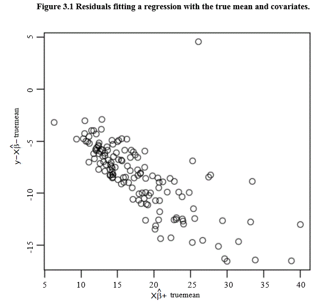
Description for Figure 3.1
Plot showing the residuals with truemean on the x-axis ranging from 5 to 40 and truemean from -15 to 5 on the y-axis to illustrate the departure from the normal distribution.
3.2 Simulation study
In
this section, we set up a simulation close to Maiti et al. (2014) (or
Sugasawa et al. (2017)) to compare the accuracy of our estimators to other
estimators, specifically those from You and Chapman (2006) and Sugasawa et al.
(2017). We generate observations for each small area from the model
where
and
Then the random effects model for the small
area mean is
where
and
Hence,
where
and
The interest parameter is the mean
for the
small area. Also, the direct estimator of
is
We
set
and
for all areas, and generate covariates
from the uniform distribution on (2, 8).
The true parameter values are set as
0.5,
0.8,
and
Also, we chose
for all simulations.
For
the MCMC implementation, we generated 5,000 posterior samples after discarding
the first 1,000 for
2,000
simulation runs. Table 3.2 provides comparison among the four models. The
comparison criteria are ASD, AAB, and BIAS, the latter being defined as
Table 3.2
Simulation result for t random effects with v = 3
Table summary
This table displays the results of Simulation result for t random effects with v = 3. The information is grouped by Model (appearing as row headers), Mean and Variance (appearing as column headers).
| Model |
Mean |
Variance |
| ASD |
AAB |
BIAS |
ASD |
AAB |
BIAS |
| RTS |
1.393 |
0.895 |
0.021 |
5.048 |
1.608 |
1.324 |
| STK |
1.821 |
0.933 |
0.025 |
5.042 |
1.514 |
1.367 |
| FH |
1.540 |
0.942 |
0.022 |
This is an empty cell |
This is an empty cell |
This is an empty cell |
| YC |
2.165 |
0.974 |
0.030 |
5.970 |
1.803 |
1.689 |
RTS
model performs better than others under ASD, AAB, and BIAS criteria for the
mean. While RTS shows small improvements over other models for AAB and BIAS
criteria, it shows approximate 23.5%, 10%, and 35.7% improvements over STK, FH
and YC models respectively for ASD criteria. For the variance, RTS and STK
models perform better than YC model.
The
following two tables provide the simulation results when one sets the degrees
of freedom as
and
Table 3.3
Simulation result for t random effects with v = 2
Table summary
This table displays the results of Simulation result for t random effects with v = 2. The information is grouped by Model (appearing as row headers), Mean and Variance (appearing as column headers).
| Model |
Mean |
Variance |
| ASD |
AAB |
BIAS |
ASD |
AAB |
BIAS |
| RTS |
1.617 |
0.949 |
0.020 |
6.569 |
1.610 |
1.070 |
| STK |
7.566 |
1.107 |
0.038 |
11.144 |
1.441 |
0.996 |
| FH |
1.921 |
1.035 |
0.022 |
This is an empty cell |
This is an empty cell |
This is an empty cell |
| YC |
9.063 |
1.187 |
0.038 |
7.072 |
1.685 |
1.340 |
Table 3.4
Simulation result for t random effects with v = 4
Table summary
This table displays the results of Simulation result for t random effects with v = 4. The information is grouped by Model (appearing as row headers), Mean and Variance (appearing as column headers).
| Model |
Mean |
Variance |
| ASD |
AAB |
BIAS |
ASD |
AAB |
BIAS |
| RTS |
1.265 |
0.862 |
0.019 |
4.876 |
1.619 |
1.428 |
| STK |
1.322 |
0.874 |
0.019 |
5.077 |
1.577 |
1.489 |
| FH |
1.350 |
0.894 |
0.020 |
This is an empty cell |
This is an empty cell |
This is an empty cell |
| YC |
1.509 |
0.905 |
0.022 |
6.201 |
1.869 |
1.802 |
With
RTS model performs better than others under
ASD, AAB, and BIAS criteria for the mean. In this simulation, the ASD values
for STK and YC models are very large compared with RTS and FH models. RTS model
shows improvements of about 78.6% over STK model, 82.2% over YC model, and 15.8%
over FH model. For AAB and BIAS, the values of RTS model are smaller than those
of other models. When considering the variance, ASD for RTS model gives
smallest value.
With
RTS model also shows better performance over
others. Especially, ASD and BIAS values indicate that RTS model improves
results when compared with STK and YC model.
The
next two tables consider the situation where one assumes normality of the
random effects. Here RTS model performs slightly worse than the other models.
Table 3.5
Simulation result for normal random effects with
Table summary
This table displays the results of Simulation result for normal random effects with . The information is grouped by Model (appearing as row headers), Mean and Variance (appearing as column headers).
| Model |
Mean |
Variance |
| ASD |
AAB |
BIAS |
ASD |
AAB |
BIAS |
| RTS |
2.896 |
1.305 |
0.038 |
6.036 |
1.512 |
0.514 |
| STK |
2.560 |
1.229 |
0.051 |
1.851 |
0.961 |
0.114 |
| FH |
2.597 |
1.240 |
0.036 |
This is an empty cell |
This is an empty cell |
This is an empty cell |
| YC |
2.735 |
1.259 |
0.048 |
3.674 |
1.305 |
0.463 |
Table 3.6
Simulation result for normal random effects with
Table summary
This table displays the results of Simulation result for normal random effects with . The information is grouped by Model (appearing as row headers), Mean and Variance (appearing as column headers).
| Model |
Mean |
Variance |
| ASD |
AAB |
BIAS |
ASD |
AAB |
BIAS |
| RTS |
3.007 |
1.316 |
0.032 |
10.117 |
1.895 |
1.202 |
| STK |
2.784 |
1.272 |
0.031 |
2.221 |
1.038 |
0.155 |
| FH |
2.765 |
1.272 |
0.048 |
This is an empty cell |
This is an empty cell |
This is an empty cell |
| YC |
2.873 |
1.285 |
0.033 |
9.166 |
1.798 |
1.129 |
