7. Simulation experiments

Isabel Molina, J.N.K. Rao and Gauri Sankar Datta

Previous | Next

A simulation study was designed with the following purposes in mind:

1. To study the properties, in terms of bias and MSE, of the PT estimators as $\alpha$  varies for fixed $A$  and as $A$  varies for fixed $\alpha .$  We would like to see which values of $\alpha$  are adequate for a given  $A.$
2. To compare the PTEs with the EBLUPs based on REML and with the EBLUPs based on AML.
3. To study the performance of the proposed MSE estimators in terms of relative bias and also in terms of coverage and length of prediction intervals.
4. To compare the three introduced small area estimators that give strictly positive weight to the direct estimator for all areas, namely EBLUP based on AML, PT-AML and REML-AML estimators.

To accomplish the above goals, data were generated from the Fay-Herriot model given by (2.1)-(2.2) with a constant mean, that is, with $p=1,\beta =\mu$  and $x_i=1,i=1,\dots \mathrm{,}m.$  We let $\mu =0$  without loss of generality, number of areas $m=15$  and $D_i=1,i=1,\dots \mathrm{,}m.$  The simulation study was repeated for increasing values of the model variance, $A\in \left\{\mathrm{0.01,0.02,0.05,0.1,0.2,1}\right\},$  and also for six significance levels of the test of $H_0:A=0$  against $H_0:A>0,$  namely $\alpha =\left\{\mathrm{0.05,0.1,0.2,0.3,0.4,0.5}\right\}.$  For each combination of $A$  and $\alpha ,$  the following steps were performed for each simulation run $\ell =1,\dots \mathrm{,}L$  with $L=\text{10,000}$  runs:

1. Generate data from the assumed model with constant zero mean; i.e.,

   $$\begin{array}{lll}{\theta }_i^{\left(\ell \right)}\hfill & =\hfill & v_i^{\left(\ell \right)}\mathrm{,}{v}_i^{\left(\ell \right)}\stackrel{\text{ind}}{\sim }N\left(\mathrm{0,}A\right)\mathrm{,}\hfill \\ y_i^{\left(\ell \right)}\hfill & =\hfill & {\theta }_i^{\left(\ell \right)}+e_i^{\left(\ell \right)}\mathrm{,}{e}_i^{\left(\ell \right)}\stackrel{\text{ind}}{\sim }N\left(\mathrm{0,}{D}_i\right)\mathrm{,}i=1,\dots \mathrm{,}m.\hfill \end{array}$$

2. Calculate the following estimators of $\theta :$  the EBLUP based on REML estimation of $A,{\widehat{\theta }}_{\text{RE}}^{\left(\ell \right)},$  the PT estimate ${\widehat{\theta }}_{\text{PT}}^{\left(\ell \right)},$  the EBLUP based on AML estimation of $A,{\widehat{\theta }}_{\text{AML}}^{\left(\ell \right)},$  the combined PT-AML estimate ${\widehat{\theta }}_{\text{PTAML}}^{\left(\ell \right)}$  and the REML-AML estimate ${\widehat{\theta }}_{\text{REAML}}^{\left(\ell \right)}.$

3. For each area $i=1,\dots \mathrm{,}m,$  calculate: the three estimates of the MSE of the EBLUP ${\widehat{\theta }}_{\text{RE},i}$  given in (3.2), (3.3) and (4.1), denoted respectively by ${\text{mse}}^{\left(\ell \right)}\left({\widehat{\theta }}_{\text{RE}\mathrm{,}i}\right),{\text{mse}}_0^{\left(\ell \right)}\left({\widehat{\theta }}_{\text{RE}\mathrm{,}i}\right)$  and ${\text{mse}}_{\text{PT}}^{\left(\ell \right)}\left({\widehat{\theta }}_{\text{RE}\mathrm{,}i}\right),$  and the three estimates (6.3), (6.4) and (6.5) of the MSE of the combined small area estimator ${\widehat{\theta }}_{\text{REAML}\mathrm{,}i},$  denoted ${\text{mse}}^{\left(\ell \right)}\left({\widehat{\theta }}_{\text{REAML}\mathrm{,}i}\right),{\text{mse}}_0^{\left(\ell \right)}\left({\widehat{\theta }}_{\text{REAML}\mathrm{,}i}\right)$  and ${\text{mse}}_{\text{PT}}^{\left(\ell \right)}\left({\widehat{\theta }}_{\text{REAML}\mathrm{,}i}\right)$  respectively.

4. For each area $i=1,\dots \mathrm{,}m,$  obtain the normality-based $1-\alpha$  prediction intervals for the small area mean ${\theta }_i$  based on the three considered MSE estimators of the EBLUP:

   $$\begin{array}{lll}{\text{CI}}_i^{\left(\ell \right)}\hfill & =\hfill & {\widehat{\theta }}_{\text{RE}\mathrm{,}i}^{\left(\ell \right)}\mp Z_{\alpha /2}\sqrt{{\text{mse}}^{\left(\ell \right)}\left({\widehat{\theta }}_{\text{RE}\mathrm{,}i}\right)}\mathrm{,}\hfill \\ {\text{CI}}_{\mathrm{0,}i}^{\left(\ell \right)}\hfill & =\hfill & {\widehat{\theta }}_{\text{RE}\mathrm{,}i}^{\left(\ell \right)}\mp Z_{\alpha /2}\sqrt{{\text{mse}}_0^{\left(\ell \right)}\left({\widehat{\theta }}_{\text{RE}\mathrm{,}i}\right)}\mathrm{,}\hfill \\ {\text{CI}}_{\text{PT}\mathrm{,}i}^{\left(\ell \right)}\hfill & =\hfill & {\widehat{\theta }}_{\text{RE}\mathrm{,}i}^{\left(\ell \right)}\mp Z_{\alpha /2}\sqrt{{\text{mse}}_{\text{PT}}^{\left(\ell \right)}\left({\widehat{\theta }}_{\text{RE}\mathrm{,}i}\right)}\mathrm{,}\hfill \end{array}$$

   where $Z_{\alpha /2}$  is the upper $\alpha /2-$ point of a standard normal distribution.

5. Repeat Steps 1-4 for $\ell =1,\dots \mathrm{,}L,$  for $L=\text{10,000}.$  Then, for each small area estimator ${\widehat{\theta }}_i\in \left\{{\widehat{\theta }}_{\text{RE}\mathrm{,}i}\mathrm{,}{\widehat{\theta }}_{\text{PT}\mathrm{,}i}\mathrm{,}{\widehat{\theta }}_{\text{AML}\mathrm{,}i}\mathrm{,}{\widehat{\theta }}_{\text{PTAML}\mathrm{,}i}\mathrm{,}{\widehat{\theta }}_{\text{REAML}\mathrm{,}i}\right\},i=1,\dots \mathrm{,}m,$  compute its empirical bias and MSE as

   $$B\left({\widehat{\theta }}_i\right)=\frac{1}{L}{\displaystyle \sum _{\ell =1}^L}\left({\widehat{\theta }}_i^{\left(\ell \right)}-{\theta }_i^{\left(\ell \right)}\right)\mathrm{,}\text{MSE}\left({\widehat{\theta }}_i\right)=\frac{1}{L}{\displaystyle \sum _{\ell =1}^L}{\left({\widehat{\theta }}_i^{\left(\ell \right)}-{\theta }_i^{\left(\ell \right)}\right)}^2\mathrm{.}$$

   Then obtain the average over areas of absolute biases and MSEs as

   $$\overline{\text{AB}}\left(\widehat{\theta }\right)=\frac{1}{m}{\displaystyle \sum _{i=1}^m}\left|B\left({\widehat{\theta }}_i\right)\right|\mathrm{,}\overline{\text{AMSE}}\left(\widehat{\theta }\right)=\frac{1}{m}{\displaystyle \sum _{i=1}^m\text{MSE}\left({\widehat{\theta }}_i\right)}\mathrm{.}$$

6. Calculate the relative bias of each MSE estimator, $\text{mse}\left({\widehat{\theta }}_i\right),$  as follows

   $$\text{RB}\left\{\text{mse}\left({\widehat{\theta }}_i\right)\right\}=\left\{\frac{1}{L}{\displaystyle \sum _{\ell =1}^L{\text{mse}}^{\left(\ell \right)}\left({\widehat{\theta }}_i\right)}-\text{MSE}\left({\widehat{\theta }}_i\right)\right\}/\text{MSE}\left({\widehat{\theta }}_i\right)\mathrm{.}$$

   Calculate the average over areas of the absolute relative biases as

   $$\overline{\text{ARB}}\left\{\text{mse}\left(\widehat{\theta }\right)\right\}=\frac{1}{m}{\displaystyle \sum _{i=1}^m\left|\text{RB}\left\{\text{mse}\left({\widehat{\theta }}_i\right)\right\}\right|}\mathrm{.}$$

7. For each type of prediction interval ${\text{CI}}_i^{\left(\ell \right)}=\left(L_i^{\left(\ell \right)}\mathrm{,}{U}_i^{\left(\ell \right)}\right),$  for ${\text{CI}}_i^{\left(\ell \right)}\in \left\{{\text{CI}}_i^{\left(\ell \right)}\mathrm{,}{\text{CI}}_{\mathrm{0,}i}^{\left(\ell \right)}\mathrm{,}{\text{CI}}_{\text{PT}\mathrm{,}i}^{\left(\ell \right)}\right\}$  given in Step 4, calculate the empirical coverage rate (CR) and the average length (AL) as

   $${\text{CR(CI}}_i)=\frac{\#\left\{{\theta }_i^{\left(\ell \right)}\in {\text{CI}}_i^{\left(\ell \right)}\right\}}{L}\mathrm{,}\text{AL}\left({\text{CI}}_i\right)=\frac{1}{L}{\displaystyle \sum _{\ell =1}^L}\left(U_i^{\left(\ell \right)}-L_i^{\left(\ell \right)}\right)\mathrm{.}$$

   Finally, average over areas the coverage rates and average lengths, as

   $$\overline{\text{CR}}\left(\text{CI}\right)=\frac{1}{m}{\displaystyle \sum _{i=1}^m\text{CR}\left({\text{CI}}_i\right)}\mathrm{,}\overline{\text{AL}}\left(\text{CI}\right)=\frac{1}{m}{\displaystyle \sum _{i=1}^m\text{AL}\left({\text{CI}}_i\right)}\mathrm{.}$$

Figures 7.1 and 7.2 plot the average MSEs of the PTEs for each $A\in \left\{\mathrm{0.05,0.1,0.2}\right\},$  together with the average MSE of the EBLUPs based on REML and AML, against the significance level $\alpha .$  Note that when $A$  is small, for large $\alpha$  the PT procedure is rejecting $H_0$  more often and therefore the PTE becomes more often the usual EBLUP, whereas for small $\alpha$  the PT procedure rejects $H_0$  less often and the regression-synthetic estimator is then more often used. In contrast, for a large value of $A,$  the PTE becomes the EBLUP more frequently regardless of $\alpha .$  The absolute biases of the estimators are not shown here because they are roughly the same for all the PTEs across $\alpha$  values. The reason for this is that when the model holds, both components of the PTE, the synthetic estimator and the EBLUP, are unbiased for the target parameter. Note that the synthetic estimator is unbiased even when $A>0.$  The first conclusion arising from Figures 7.1 and 7.2 is that the MSE of the PTE is practically constant across $\alpha \ge \mathrm{0.1.}$  See also that the average MSE of the PTE for a given $\alpha$  increases with $A$  because the PTE reduces to the EBLUP more often as $A$  increases and the MSE of the EBLUP increases with $A.$  Observe also that the PTE and the EBLUP based on REML perform very similarly for $\alpha \ge \mathrm{0.2.}$  However, for $\alpha <0.2,$  the PTE becomes more efficient than the EBLUP as soon as $A$  moves close to the null hypothesis $\left(A<0.1\right),$  which agrees with the remark of Datta et al. (2011).

Turning to the EBLUP based on AML, Figures 7.1 and 7.2 show that its average MSE is significantly larger than that of the other two estimators, but the differences with the other ones decrease as $A$  increases. This is due to bias of the AML estimator of $A$  for small $A.$  We shall study later the combined small area estimators PT-AML and REML-AML, which use the EBLUP based on AML only when null hypothesis is not rejected or when the realized estimate of $A$  is zero.

Figure 7.1 Average MSEs of PTE, EBLUP based on REML and EBLUP based on AML against $\alpha ,$  for a) $A=0.05$  and b) $A=\mathrm{0.1.}$

Description for Figure 7.1

Datta et al. (2011, page 366) recommended $\alpha \ge 0.2$  for the PTE. Moreover, the literature on PT estimation for fixed effects models suggests that a good choice of $\alpha$  in terms of bias and MSE is $\alpha =0.2$  (Bancroft 1944; Han and Bancroft 1968). But the above results suggest that for $\alpha \ge 0.2,$  the PTE is practically the same as the EBLUP and therefore one might choose to always use the EBLUP.

Figure 7.2 Average MSEs of PTE, EBLUP based on REML and EBLUP based on AML against $\alpha ,$  for $A=\mathrm{0.2.}$ $$

Description for Figure 7.2

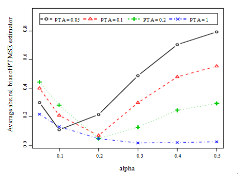
Now we study the properties of the PT for MSE estimation in terms of $\alpha .$  Figure 7.3 plots the average absolute relative bias of the MSE estimators ${\text{mse}}_{\text{PT}}\left({\widehat{\theta }}_{\text{RE}\mathrm{,}i}\right)$  labelled PT, against the significance level $\alpha ,$  for each value $A\in \left\{\mathrm{0.05,0.1,0.2,1}\right\}.$  When $\alpha$  is taken very small $\alpha <0.1,$  the null hypothesis $H_0:A=0$  is less often rejected and ${\text{mse}}_{\text{PT}}\left({\widehat{\theta }}_{\text{RE}\mathrm{,}i}\right)$  becomes often $g_{2i},$  which leads to underestimation. For $\alpha$  large $\left(\alpha >0.2\right),$  the null hypothesis is more often rejected and ${\text{mse}}_{\text{PT}}\left({\widehat{\theta }}_{\text{RE}\mathrm{,}i}\right)$  becomes the usual MSE estimator of the EBLUP, which severely overestimates the true MSE for small $A.$  The value $\alpha =0.2$  appears to be a good compromise choice, with an average absolute relative bias around 10% for $A\ge 0.1$  and 20% for $A=\mathrm{0.05.}$

Figure 7.3 Average over areas of absolute relative biases of the MSE estimator ${\text{mse}}_{\text{PT}}\left({\widehat{\theta }}_{\text{RE}\mathrm{,}i}\right),$  labelled PT, for $A\in \left\{\mathrm{0.05,0.1,0.2,1}\right\}$  against significance level $\alpha .$

Description for Figure 7.3

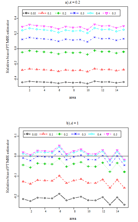
The above results suggest that $\alpha =0.2$  is a good choice when using the PT procedure to estimate the MSE of the usual EBLUP. This has been more thoroughly studied by looking at the (signed) relative biases of ${\text{mse}}_{\text{PT}}\left({\widehat{\theta }}_{\text{RE}\mathrm{,}i}\right)$  for each area. These results are plotted in Figures 7.4 and 7.5 with four plots, one for each value of $A\in \left\{\mathrm{0.05,0.1,0.2,1}\right\}.$  The figures appearing in the legends of these plots are the significance levels $\alpha$  for the PT MSE estimator ${\text{mse}}_{\text{PT}}\left({\widehat{\theta }}_{\text{RE}\mathrm{,}i}\right).$  These plots confirm our previous observations: the MSE estimator based on the PT, ${\text{mse}}_{\text{PT}}\left({\widehat{\theta }}_{\text{RE}\mathrm{,}i}\right),$  underestimates $\text{MSE}\left({\widehat{\theta }}_{\text{RE}\mathrm{,}i}\right)$  for small $\alpha$  and overestimates for large $\alpha .$  It turns out that ${\text{mse}}_{\text{PT}}\left({\widehat{\theta }}_{\text{RE}\mathrm{,}i}\right)$  with $\alpha =0.2$  is a good candidate for all values of $A.$

Figure 7.4 Relative biases of ${\text{mse}}_{\text{PT}}\left({\widehat{\theta }}_{\text{RE}\mathrm{,}i}\right),$  for each significance level $\alpha \in \left\{\mathrm{0.05,0.1,0.2,0.3,0.4,0.5}\right\},$  against area $i,$  for a) $A=0.05$  and b) $A=\mathrm{0.1.}$

Description for Figure 7.4

Figure 7.5 Relative biases of ${\text{mse}}_{\text{PT}}\left({\widehat{\theta }}_{\text{RE}\mathrm{,}i}\right),$  for each significance level $\alpha \in \left\{\mathrm{0.05,0.1,0.2,0.3,0.4,0.5}\right\},$  against area $i,$  for a) $A=0.2$  and b) $A=1.$

Description for Figure 7.5

Let us now compare ${\text{mse}}_{\text{PT}}\left({\widehat{\theta }}_{\text{RE}\mathrm{,}i}\right)$  for the selected significance level $\alpha =0.2$  with the other two MSE estimators ${\text{mse}}_0\left({\widehat{\theta }}_{\text{RE}\mathrm{,}i}\right)$  and $\text{mse}\left({\widehat{\theta }}_{\text{RE}\mathrm{,}i}\right)$  given by (3.3) and (3.2) respectively. Figure 7.6 plots the average absolute relative biases of the three MSE estimators, labelled respectively PT, REML0 and REML. We note that ${\text{mse}}_0\left({\widehat{\theta }}_{\text{RE}\mathrm{,}i}\right)$  performs better than $\text{mse}\left({\widehat{\theta }}_{\text{RE}\mathrm{,}i}\right)$  for all areas, but still ${\text{mse}}_{\text{PT}}\left({\widehat{\theta }}_{\text{RE}\mathrm{,}i}\right)$  is better than ${\text{mse}}_0\left({\widehat{\theta }}_{\text{RE}\mathrm{,}i}\right)$  for all considered values of $A$  except for $A=1,$  where the differences between the three estimators are negligible. The differences decrease as $A$  increases, but observe that the usual MSE estimator, $\text{mse}\left({\widehat{\theta }}_{\text{RE}\mathrm{,}i}\right),$  can be severely biased for small $A,$  with an average absolute relative bias over 50% for $A<0.2$  and exponentially growing as $A$  tends to zero. The conclusion is that, when $H_0$  is not rejected, even if the realized estimate of $A$  is positive, it seems better to omit the $g_{3i}$  term in the MSE estimator and consider only $g_{2i}.$

Figure 7.6 Average over areas of absolute relative biases of MSE estimators ${\text{mse}}_{\text{PT}}\left({\widehat{\theta }}_{\text{RE}\mathrm{,}i}\right)$  with $\alpha =0.2,$  labelled PT, $\text{mse}\left({\widehat{\theta }}_{\text{RE}\mathrm{,}i}\right)$  labelled REML and ${\text{mse}}_0\left({\widehat{\theta }}_{\text{RE}\mathrm{,}i}\right)$  labelled REML0, against $A.$

Description for Figure 7.6

We now turn to the small area estimators that attach strictly positive weight to the direct estimator for all areas: EBLUP based on AML, ${\widehat{\theta }}_{\text{AML}},$  and the two combined estimators, PT-AML given in (6.1), and REML-AML given in (6.2). Average MSEs are plotted in Figure 7.7 for these three estimators. In this plot, ${\widehat{\theta }}_{\text{AML}}$  seems to be a little less efficient, followed by PT-AML. The combined estimator REML-AML seems to perform slightly better than its two counterparts for small $A,$  although for $A\ge 0.2$  the PT-AML estimator is very close to it. For MSE estimation, we focus on REML-AML because of its better performance.

Figure 7.7 Average over areas of MSEs of PT-AML estimator with $\alpha =0.2,$  EBLUP based on AML and REML-AML estimator against $A.$

Description for Figure 7.7

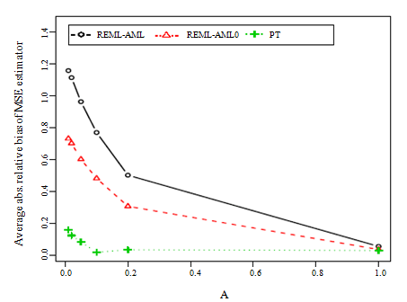
For the combined estimator REML-AML, Figure 7.8 shows that the MSE estimator based on the PT, ${\text{mse}}_{\text{PT}}\left({\widehat{\theta }}_{\text{REAML}\mathrm{,}i}\right),$  which uses only $g_{2i}$  whenever ${\widehat{A}}_{\text{RE}}=0$  or the null hypothesis is not rejected, has average absolute relative bias less than 10% for $A\ge 0.1$  and it is smaller than the corresponding values for $\text{mse}\left({\widehat{\theta }}_{\text{REAML}\mathrm{,}i}\right)$  and ${\text{mse}}_0\left({\widehat{\theta }}_{\text{REAML}\mathrm{,}i}\right),$  especially for $A\le \mathrm{0.4.}$

Figure 7.8 Average over areas of absolute relative biases of the MSE estimators $\text{mse}\left({\widehat{\theta }}_{\text{REAML}\mathrm{,}i}\right),$   ${\text{mse}}_0\left({\widehat{\theta }}_{\text{REAML}\mathrm{,}i}\right)$  and ${\text{mse}}_{\text{PT}}\left({\widehat{\theta }}_{\text{REAML}\mathrm{,}i}\right),$  labelled respectively REML-AML, REML-AML0 and PT, against $A.$

Description for Figure 7.8

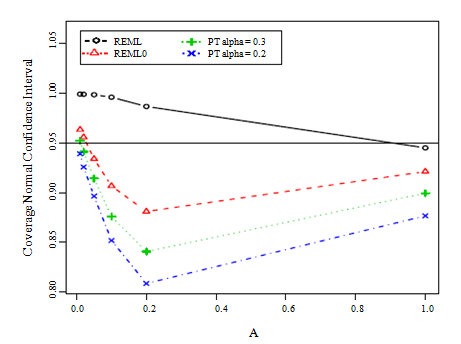
Finally, we analyze the average over areas of coverage rates and average lengths of normality-based prediction intervals for the small area mean ${\theta }_i$  using the EBLUP based on REML as point estimate and the three different MSE estimators of the EBLUP, namely $\text{mse}\left({\widehat{\theta }}_{\text{RE}\mathrm{,}i}\right),{\text{mse}}_0\left({\widehat{\theta }}_{\text{RE}\mathrm{,}i}\right)$  and ${\text{mse}}_{\text{PT}}\left({\widehat{\theta }}_{\text{RE}\mathrm{,}i}\right).$  Figure 7.9 shows the coverage rates of these three types of intervals, where the MSE estimators based on the PT procedure were obtained taking $\alpha =0.2,\mathrm{0.3.}$  It seems that the good relative bias properties of the MSE estimator based on the PT, ${\text{mse}}_{\text{PT}}\left({\widehat{\theta }}_{\text{RE}\mathrm{,}i}\right),$  for small $A$  cannot be extrapolated to coverage based on normal prediction intervals, showing undercoverage especially for $A=\mathrm{0.2.}$  In this case, taking a larger significance level $\alpha =0.3$  reduces a little the undercoverage of the prediction intervals obtained using ${\text{mse}}_{\text{PT}}\left({\widehat{\theta }}_{\text{RE}\mathrm{,}i}\right).$  Still, the coverage rates of ${\text{mse}}_0\left({\widehat{\theta }}_{\text{RE}\mathrm{,}i}\right)$  are better for all values of $A.$  As expected, the usual MSE estimator $\text{mse}\left({\widehat{\theta }}_{\text{RE}\mathrm{,}i}\right)$  provides overcoverage for small values of $A,$  which is due to the severe overestimation of the MSE. On the other hand, the intervals showing undercoverage also lead to shorter prediction intervals as shown by Figure 7.10.

It is worthwhile to mention that the construction of prediction intervals for ${\theta }_i$  based on the Fay-Herriot model with accurate coverage rates is not an obvious task. Several papers have appeared in the literature for this problem. For example, Chatterjee, Lahiri and Li (2008) proposed prediction intervals with second order correct coverage rate using only the $g_{1i}$  term as MSE estimate and applying a bootstrap procedure to find the calibrated quantiles. Diao, Smith, Datta, Maiti and Opsomer (2014) have recently obtained prediction intervals with second order correct coverage rate avoiding the use of resampling procedures and using the full MSE estimator. Obtaining prediction intervals with accurate coverage using other MSE estimates is still a challenge and it is out of scope of this paper.

Figure 7.9 Average over areas of coverage rates of normality-based prediction intervals for ${\theta }_i$  using the MSE estimators $\text{mse}\left({\widehat{\theta }}_{\text{RE}\mathrm{,}i}\right),{\text{mse}}_0\left({\widehat{\theta }}_{\text{RE}\mathrm{,}i}\right)$  and ${\text{mse}}_{\text{PT}}\left({\widehat{\theta }}_{\text{RE}\mathrm{,}i}\right)$  with $\alpha =0.2,0.3,$  labelled respectively REML, REML0 and PT, against $A.$

Description for Figure 7.9

Figure 7.10 Average over areas of average lengths of normality-based intervals for ${\theta }_i$  using the MSE estimators $\text{mse}\left({\widehat{\theta }}_{\text{RE}\mathrm{,}i}\right),{\text{mse}}_0\left({\widehat{\theta }}_{\text{RE}\mathrm{,}i}\right)$  and ${\text{mse}}_{\text{PT}}\left({\widehat{\theta }}_{\text{RE}\mathrm{,}i}\right)$  with $\alpha =0.2,0.3,$  labelled respectively REML, REML0 and PT, against $A.$

Description for Figure 7.10

This simulation study described above was repeated for several patterns of unequal sampling variances $D_i.$  Although results are not reported here, conclusions are very similar as long as the variance pattern is not extremely uneven.

Previous | Next